Worst-case Guarantees for Remote Estimation of an Uncertain Source
Mukul Gagrani, Yi Ouyang, Mohammad Rasouli, Ashutosh Nayyar

TL;DR
This paper addresses a worst-case scenario for remote estimation of an uncertain autoregressive source with bounded noise, establishing optimal open-loop communication schedules and estimation strategies under limited communication.
Contribution
It provides a complete characterization of optimal strategies for a decentralized minimax problem in remote estimation with bounded noise.
Findings
Optimal open-loop communication scheduling strategy identified.
The optimal estimator depends only on the most recent received observation.
Complete solution to the decentralized minimax decision problem.
Abstract
Consider a remote estimation problem where a sensor wants to communicate the state of an uncertain source to a remote estimator over a finite time horizon. The uncertain source is modeled as an autoregressive process with bounded noise. Given that the sensor has a limited communication budget, the sensor must decide when to transmit the state to the estimator who has to produce real-time estimates of the source state. In this paper, we consider the problem of finding a scheduling strategy for the sensor and an estimation strategy for the estimator to jointly minimize the worst-case maximum instantaneous estimation error over the time horizon. This leads to a decentralized minimax decision-making problem. We obtain a complete characterization of optimal strategies for this decentralized minimax problem. In particular, we show that an open loop communication scheduling strategy is optimal…
Click any figure to enlarge with its caption.
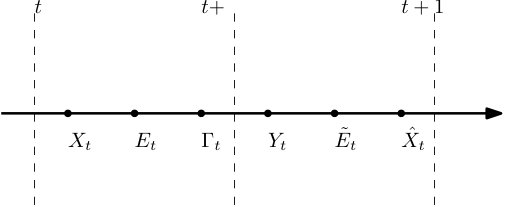 Figure 1
Peer Reviews
No public reviews on file for this paper yet. If you reviewed it on a platform where reviews are public (OpenReview, ICLR, NeurIPS, ICML), you can paste yours below so the community can read it here.
Videos
No videos yet. Explain this paper in a talk, walkthrough, or lecture? Add one.
Worst-case Guarantees for Remote Estimation of an Uncertain Source
Mukul Gagrani, Yi Ouyang, Mohammad Rasouli and Ashutosh Nayyar This work was supported by NSF Grant ECCS 1509812, CNS 1446901 and ECCS 1750041.
Abstract
Consider a remote estimation problem where a sensor wants to communicate the state of an uncertain source to a remote estimator over a finite time horizon. The uncertain source is modeled as an autoregressive process with bounded noise. Given that the sensor has a limited communication budget, the sensor must decide when to transmit the state to the estimator who has to produce real-time estimates of the source state. In this paper, we consider the problem of finding a scheduling strategy for the sensor and an estimation strategy for the estimator to jointly minimize the worst-case maximum instantaneous estimation error over the time horizon. This leads to a decentralized minimax decision-making problem. We obtain a complete characterization of optimal strategies for this decentralized minimax problem. In particular, we show that an open loop communication scheduling strategy is optimal and the optimal estimate depends only on the most recently received sensor observation.
I Introduction
Information collection is essential for most engineering systems. In many applications, sensors are deployed to collect and send information to a base station/control center to estimate or control the state of the system. In environmental monitoring, for example, remote sensors are used to measure environmental variables such as temperature, rainfall, soil moisture, etc. The sensors collect information and transmit it to the base station through wireless communication. For a sensor with limited battery, the energy spent in communication is a significant factor determining the battery lifespan. Since battery replacement is expensive for remote sensors, it is important for sensors to adopt a transmission schedule that preserves energy while achieving a desired level of estimation accuracy. Similar scenarios of remote estimation also arise in other applications such as smart grids, networked control systems and healthcare monitoring [1, 2, 3].
The remote estimation problem with one sensor and one estimator has been studied under two different communication models: i) Remote estimation with pull communication protocol: In this class of problems the estimator decides when to get data from the sensor. Since the estimator is the only decision-maker in the system, this protocol leads to a centralized sequential decision-making problem. Instances of such problems have been studied in [4, 5, 6, 7]. ii) Remote estimation with push communication protocol: Here, the sensor makes the decision about when to send data to the estimator. The estimator decides, at each time, what estimate to produce. This leads to a decentralized decision-making problem with the sensor and the estimator as the two decsion-makers. Computing jointly optimal scheduling and estimation strategies in a decentralized setup is difficult in general. However, several works have addressed this problem by placing some restrictions on the transmission/estimation strategies and/or by making certain assumptions about the source statistics. For example, [8, 9] studied the problem of remote estimation under limited number of transmissions when the state process is i.i.d. and the transmission strategy is restricted to be threshold-based. A continuous-time version of the problem is considered in [10] with a Markov state process, limited number of transmissions and a fixed estimation strategy. [11] derived the optimal communication schedule assuming a Kalman-like estimator. Jointly optimal scheduling and estimation strategies were derived in [12, 13, 14] for Markov sources that satisfied certain symmetry assumptions on their probability distributions.
The uncertainties in all the aforementioned work are modeled as random variables and the objective is to minimize the expected sum cost over a finite time horizon. However, in many applications, there is no statistical model for the system variables of interest. Furthermore, guarantees on estimation accuracy at each time instant may be critical for safety concerned systems such as healthcare monitoring. For example, while monitoring the heartbeat of a patient it is desirable that the estimation error at each time is minimal.
In this paper, we consider an uncertain source that can be modeled as a discrete-time autoregressive process with bounded noise. The source is observed by a sensor with limited communication budget. The sensor can communicate with a remote estimator that needs to produce real-time estimates of the source state. Given such a model, we are interested in the worst-case guarantee on estimation error at any time that can be achieved under a limited communication budget. Put another way, we want to find the minimum communication budget needed to ensure that the worst-case estimation error at any time is below a given threshold. In order to address these questions, we consider a minimax formulation of the remote estimation problem. Our goal is to design a communication scheduling strategy for the sensor and an estimation strategy for the estimator to jointly minimize the worst-case instantaneous estimation cost over all realizations of the source process.
Centralized decision and control problems where the goal is to minimize a worst-case cost have long been studied in the literature. One prominent line of work has focused on developing dynamic program type approaches for minimax problems [15, 16, 17, 18, 19]. These centralized minimax dynamic programs use analogues of stochastic dynamic programming concepts such as information states and value functions. The centralized minimax dynamic program can be interpreted in terms of a zero-sum game between the controller and an adversary who selects the disturbances to maximize the cost metric [15, 16]. Dynamic games based approaches for minimax design problems were also studied in [20]. Minimax problems where the goal is to minimize the worst-case maximum instantaneous cost were studied in [21, 22, 23].
In the centralized minimax problems described above, the uncertainties are described in terms of the set of values they can take. In contrast, some minimax problems have looked at systems with stochastic uncertainties. In these problems, the parameters of the stochastic uncertainties are ambiguous. These parameters are either fixed apriori but unknown or they are chosen dynamically by an adversary. In either case, the objective of the control problem is to minimize the maximum expected cost corresponding to the worst-choice of unknown parameters. Examples of this line of work include [24, 25, 26, 27, 28].
Our minimax problem is most closely related to the minimax control problems studied in [15] and [22, 23]. The minimax problems in [15] and [22, 23] were centralized decision-making problem involving a single decision-maker acting over time. In contrast, our minimax problem involves two decision-makers, the sensor and the estimator, making decisions based on different information. The decentralized nature of our decision problem creates issues such as signaling where decision-makers may communicate implicitly through their actions. A decision to not communicate by the sensor, for example, can implicitly convey some information about the source to the estimator. Such signaling effects are a key reason why the joint optimization of strategies becomes a difficult problem [12, 13]. A class of decentralized minimax control problems with partial history sharing were investigated in [29].
In order to jointly optimize the strategies for the sensor and the estimator while taking into account the signaling between them, we extend the coordinator-based approach of [30], [13] which was developed for a stochastic model and expected cost criterion to our minimax setting. Using this, we explicitly identify optimal communication scheduling and estimation strategy for our minimax problem.
Organization: We start with a general centralized minimax control problem in Section II and then formulate the minimax remote estimation problem in Section III. We formulate an equivalent centralized minimax control problem in Section IV and derive the optimal scheduling and estimation strategies in Section V. We conclude in Section VI.
Notation and Uncertain Variables: denotes the collection of variables . denotes the indicator function of an event .
We now review the concept of uncertain variables as defined in [31]. An uncertain variable is a mapping from some underlying sample space to a space of interest. We use capital letters to denote uncertain variables while small letters denote their realizations and script letters denote the spaces of all possible realizations. For example, an uncertain variable has a realization for an outcome .
Instead of probability measures as in the case of random variables, uncertain variables can be analyzed using their ranges. The range of is defined as . Similarly, for a collection of uncertain variables , . The conditional range of given is denoted by (or ) and is defined as . We also define the uncertain conditional range as an uncertain variable that takes the value when takes the value .
Using the ranges of uncertain variables, an analogue of statistical independence can be defined as follows [Definition 2.1 [31]].
Definition 1**.**
Uncertain variables are unrelated if
[TABLE]
where is the Cartesian product.
The following property comes from the definition of unrelated uncertain variables [Lemma 2.1 [31]].
Property 1**.**
If is unrelated to , that is, , then
[TABLE]
For a function , we define to denote its supremum over the range of . Similarly . Also, denotes the supremum of over the conditional range. For a bivariate function , we have the following property.
Property 2**.**
If are uncertain variables. Then
[TABLE]
Furthermore, if is another uncertain variable, then
[TABLE]
Note that the above property is the analogue of the tower property of conditional expectation with supremum playing the role of expectation.
II Minimax Control with Maximum Instantaneous Cost Objective
Consider a discrete time system with state and observation evolving according to the following dynamics:
[TABLE]
where is the control action, is the noise, , and . The noise process is a sequence of unrelated uncertain variables. We assume that the state has two components, , where is the hidden part and is the observable part.
At each time , the controller’s available information is . Note that includes the history of observations , the history of observable part of the states and the past control actions . denotes the set of all possible values of . The set of available control actions at , which may depend on the directly observable state , is . Based on the available information at , the controller takes a control action according to a function as
[TABLE]
We call a strategy of the controller. The instantaneous cost at time is . The minimax control objective is to find a strategy that minimizes the worst-case maximum instantaneous cost. Thus, the strategy optimization problem is
[TABLE]
Let be the conditional range of the hidden part of the state given the available information . Let denote the space of all possible . Note that belongs to , so conditional range of given is the singleton set i.e. .
The conditional range along with can be used as an information state for decision-making in the minimax control problem. In particular, we can obtain the following dynamic programming result using arguments from [23].
Theorem 1**.**
*For each , define functions as follows:
i) For ,*
[TABLE]
ii) For ,
[TABLE]
where is given as follows,
[TABLE]
If the infimum in (9), (10) is achieved, then for each and the minimizing in (9)-(10) gives the optimal action at time for . Moreover, the optimal cost is given by .
Proof.
See Appendix A ∎
III Problem Formulation
Consider a communication problem between a sensor (transmitter) and an estimator (receiver) over a finite time horizon , . The sensor perfectly observes a discrete-time uncertain process which evolves according to the following dynamics
[TABLE]
where is a scalar and is an orthogonal matrix. is an uncertain variable which lies in the ball of radius around the origin i.e. . We assume that the initial state . The numbers are finite. Since all the noise in the system is bounded, the state also remains bounded for all . Let denote a bounded set such that for .
The sensor can send the observed state to the estimator through a perfect channel. However, each transmission consumes one unit of sensor’s energy, and the sensor has a limited energy budget of units111 is a fixed known integer and not an uncertain variable with . Let denote the energy available at time . We use to denote the transmission decision at time . is if the current state observation is transmitted and [math] otherwise. Note that where if and i.e. there can be no transmission at time if . The energy at time can be written as:
[TABLE]
The estimator receives at time which is given as,
[TABLE]
where denotes no transmission. The sensor makes the transmission decision at based on available information ,
[TABLE]
where is the transmission strategy of the sensor at time . We call the collection the transmission strategy.
The estimator produces an estimate of the state based on its received information at time as follows:
[TABLE]
where denotes the estimation strategy at time . The collection is referred to as the estimation strategy. The cost incurred under a transmission strategy and estimation strategy is the worst case maximum instantaneous distortion cost over the entire horizon, given by,
[TABLE]
We can now formulate the following problem.
Problem 1**.**
Determine a transmission strategy for the sensor and an estimation strategy for the estimator which jointly minimize the cost in (16).
[TABLE]
Remark 1**.**
Communication scheduling and remote estimation problems similar to Problem 1 have been studied in [9, 12, 13]. The key differences between the problems in [9, 12, 13] and Problem 1 are: (i) source model- [9, 12, 13] deal with a stochastic source model whereas the source model in Problem 1 is non-stochastic; (ii) objective- [9, 12, 13] deal with minimizing an expected cumulative cost over a time horizon whereas the objective in Problem 1 is to minimize the worst-case instantaneous cost. The objective in Problem 1 may be more suitable for safety critical systems.
Next, we provide a structural result which establishes that the sensor can ignore past values of the source and energy levels without losing performance.
Lemma 1**.**
The transmission strategy can be restricted to the form without any loss in performance.
Proof.
See Appendix B. ∎
Problem 1 is a minimax sequential decision-making problem with two decision-makers (the sensor and the estimator). We will adopt the common information approach [13] for stochastic remote estimation problem to our minimax problem. This involves formulating a single-agent sequential decision-making problem from the perspective of an agent who knows the common information. In our setup, we can adopt the estimator’s perspective to formulate the single-agent problem as done in the following section.
IV An Equivalent Problem
We now formulate a new sequential decision problem that will help us to solve Problem 1. In the new problem, we consider the model of Section III with the following modification. At the beginning of time step, the estimator selects a mapping . will be referred to as the estimator’s prescription to the sensor. The sensor uses the prescription to evaluate as follows:
[TABLE]
The estimator selects the prescription based on its available information, that is,
[TABLE]
where the function is referred to as the prescription strategy at time . At the end of time step, the estimator produces an estimate as follows
[TABLE]
where is the estimation strategy at time . The cost incurred by the prescription strategy and the estimation strategy is,
[TABLE]
We consider the following problem,
Problem 2**.**
Determine a prescription strategy and an estimation strategy to minimize the cost .
[TABLE]
In Problem 2, the estimator is the sole decision-maker since the sensor merely evaluates the prescription at the current source state. Problem 2 can be shown to be equivalent to Problem 1 in a similar manner as in [13] for the stochastic remote estimation problem. The main idea is that for every choice of sensor strategy there exists an equivalent prescription strategy and vice-versa. Since this equivalence is true for every realization of the uncertain variables , the stochastic case argument also holds in this minimax scenario.
Problem 2 can be seen as an instance of the minimax problem formulated in Section II as follows:
We can imagine the system operating with decision points by splitting each time instant into two decision points: (i) At each time , before the transmission at that time the estimator decides the prescription ; (ii) After receiving , the estimator decides . We denote this decision point by (See Figure 2).
State: At , the state is since is observable by the estimator. At , where is the post-transmission energy given as
[TABLE] 3. 3.
Actions : At , action , where is the collection of functions from to . Recall that and for . At , action . 4. 4.
Information: The information available at time to choose a prescription is and at time to generate is . 5. 5.
Cost: The instantaneous cost at time , and at time , .
Since Problem 2 is an instance of the minimax problem of Section II, we can use Theorem 1 to conclude that the optimal strategy is a function of the conditional range of the state given the estimator’s information. Since is known to the estimator, we just need to define the conditional range of . For that purpose, we define as the pre-transmission conditional range of and as the post-transmission conditional range of at time as follows:
[TABLE]
The following lemma describes the evolution of the sets and .
Lemma 2**.**
The pre-transmission conditional range at time is a function of i.e. . 2. 2.
The post-transmission conditional range is a function of and i.e. .
Proof.
Given the post-transmission conditional range , is given as
[TABLE] 2. 2.
Given the pre-transmission conditional range , can be evaluated after receiving as follows
[TABLE]
∎
Let denote the space of all possible realizations of and . Then, Theorem 1 can be used to write a dynamic program which characterizes the optimal estimates and the optimal prescriptions in Problem 2 as follows,
Lemma 3**.**
*For , define the functions and as follows:
(i) For and define222 denotes a realization of the post-transmission energy as defined in (20).,*
[TABLE]
(ii) For , and define,
[TABLE]
*where .
(iii) For , and define,*
[TABLE]
Suppose the infimum in (23),(24),(25) are always achieved. Then, for each and the minimizing in (24) gives the optimal prescription at time . Also, for each (or ), the minimizing gives the optimal estimate. Furthermore, is the optimal cost for Problem 2.
Proof.
The result follows by writing the dynamic program using Theorem 1, Lemma 2 and associating the function with the value function at time and with the value function at time . ∎
Note that the above dynamic program is computationally hard to solve because: i) It involves minimization over functions in (24) ii) The information state is the conditional range of the source state and thus can be any arbitrary subset of . In the next section, we will analyze the dynamic program to obtain certain properties of the value functions which will help us in identifying the structure of the optimal strategies.
V Globally optimal strategies
We now proceed with solving the dynamic program of Lemma 3. We proceed in four steps.
Step 1: Nature of optimal prescriptions
We define a relation between sets which will be helpful in identifying the structure of the globally optimal prescriptions. To that end, we define the radius of a set as . The following lemma gives the relation between the radius of a set and the radius of its transformation defined by (1).
Lemma 4**.**
Let . Then,
[TABLE]
Proof.
See Appendix C. ∎
We now define a relation between sets and a property for functions.
Definition 2**.**
Let be two sets. We say if . 2. 2.
We say that a function satisfies property if
[TABLE]
Let denote the ’always transmit’ prescription, i.e. . Let denote the ’never transmit’ prescription, i.e. .
Lemma 5**.**
For each , the functions and of Lemma 3 satisfy property . 2. 2.
For each , either or is an optimal choice of prescription in (24).
Proof.
See Appendix C. ∎
Consider two singleton sets and . The first part of Lemma 5 implies that because . Thus, does not depend on the value of and can be represented as function of energy alone, that is, . The second part of Lemma 5 implies that we can replace the infimum in (24) by minimzation over just two prescriptions, and . Using the above observations, we can reduce the dynamic program of Lemma 3 to the following:
[TABLE]
where (27) and (28) follow from the definition of and the dynamic program in Lemma 3; for ,
[TABLE]
where for any . For ,
[TABLE]
Step 2: Simplified information state
We will now use property to simplify the information state of the dynamic program. Lemma 5 suggests that value functions depend only on the radius of the conditional range. Thus, we would expect that the radius of the conditional range can act as an information state of the dynamic program. This idea is formalized in the following lemma.
Lemma 6**.**
*Define and as follows:
(i) For , and ,*
[TABLE]
(ii) For , and ,
[TABLE]
(iii) For ,
[TABLE]
Then, for ,
[TABLE]
Proof.
follows from (31), (27). We then proceed by induction — we first show that (35) is true if (34) is true for . (35) follows easily from (29),(30) and the induction hypothesis by noting that . Next, we show that (34) is true for if (35) is true for . Using (28) and the induction hypothesis together with the fact that , (34) can be easily established. ∎
We can further eliminate from (31)-(33) to obtain a recursive relation among given as:
[TABLE]
For ,
[TABLE]
The above equations can be seen as a reduced version of the dynamic program of Lemma 3 with the radius of the conditional range and the energy level as the information state. Unlike the dynamic program of Lemma 3, however, the above dynamic program is completely deterministic, that is, it does not involve maximization over any uncertain variables. In the next step, we will connect this deterministic dynamic program to a deterministic optimal control problem and use it to identify optimal transmission strategy.
**Step 3: A deterministic control problem
**Consider a deterministic control system with state and control action , where if and , operating for a time horizon . The dynamics of the state are as follows:
[TABLE]
with and . The instantaneous cost is given by
[TABLE]
The deterministic control problem can be stated as follows.
Problem 3**.**
Determine a control sequence to minimize the cost
[TABLE]
We are interested in the above deterministic control problem because of the following lemma.
Lemma 7**.**
The optimal cost for the original problem (i.e, Problem 1), the coordinator’s problem (i.e, Problem 2) and the deterministic control problem (i.e, Problem 3) are equal. That is,
[TABLE]
Proof.
We have already discussed that Problems 1 and 2 are equivalent, so we will focus on the second equality in (38). Since the deterministic control problem is a special case of the minimax problem of Section II, we can use Theorem 1 to write the following dynamic program for it:
[TABLE]
for ; with being the optimal cost for Problem 3.
Comparing the above dynamic program with (36)-(37), it is easy to see that . From Theorem 1, the optimal cost of Problem 3 is
[TABLE]
which is the same as the optimal cost of Problem 2.
∎
**Step 4: Optimal transmission and estimation strategies for Problem 1 ** - We can now identify optimal transmission and estimation strategies for Problem 1. We start with the estimation strategy. We define and for ,
[TABLE]
Lemma 8**.**
In Problem 1 and Problem 2, the globally optimal estimation strategy is , for .
Proof.
See Appendix D. ∎
Let be an optimal open loop control sequence for Problem 3. Since Problem 3 is an optimal control problem with determinstic dynamics we know that there exists such an open loop strategy and can be computed via the dynamic program. We can now identify the optimal strategies for Problem 1.
Theorem 2**.**
Let be the estimation strategy as defined in Lemma 8 and be defined as follows:
[TABLE]
where is an optimal open loop control sequence for Problem 3. Then, are globally optimal strategies for Problem 1.
Proof.
See Appendix D. ∎
Theorem 2 establishes that the globally optimal transmission strategy to minimize the worst-case instantaneous cost is an open-loop strategy that transmits at pre-determined time instants. Thus, even though the sensor has access to the state and transmission history, this information is not used by the optimal transmission strategy.
Remark 2**.**
We can compare the nature of optimal strategies in Theorem 2 with the optimal strategies in the stochastic remote estimation problem in [13, 12]. The optimal estimation strategy obtained in our minimax setup is identical to the one obtained in the stochastic case considered in [13, 12]. However, the optimal transmission strategy in [13, 12] is a threshold-based strategy in contrast to the deterministic strategy obtained in our setup.
V-A Homogenous noise
Consider the case when all the uncertain noise variables take values in the ball of same size i.e for all . It turns out that transmitting at uniformly spaced intervals is optimal in this case as made precise in the following lemma.
Lemma 9**.**
Define . Then,
The optimal cost for Problem 1 under homogenous noise model is,
[TABLE] 2. 2.
An optimal control sequence for Problem 1 under homogenous noise model is given as follows:
[TABLE]
Proof.
See Appendix E. ∎
Remark 3**.**
In the case of homogenous noise, it is possible that the sensor does not utilize all the available transmission opportunities under the transmission strategy . For example, when , the sensor will transmit only twice at . Thus, the worst-case error achieved in this case would be the same even if . Therefore, one could also ask the following question: What is the minimum number of transmission opportunities () required so that the worst-case error is at most ? can be computed as follows:
[TABLE]
Remark 4**.**
Consider the problem where the estimator requests transmissions instead of the sensor deciding when to transmit. The cost of this problem is lower bounded by the cost of Problem 1 because the sensor has more information to make the transmission decision than the estimator. Moreover, since the optimal scheduling strategy obtained for Problem 1 is an open loop strategy, it can also be implemented in this new problem. Therefore, the results obtained for Problem 1 also hold for this problem.
Remark 5**.**
Consider the problem where the sensor can observe the source state only times instead of observing the state at each time with . In addition to the scheduling strategy, here the sensor must also decide when to observe the source. The cost of this problem is lower bounded by the cost of Problem 1 because the sensor has less information in this case compared to Problem 1. Also, since the optimal scheduling strategy for Problem 1 is an open loop strategy, the sensor in this problem can take observations at the fixed times when it transmits, thereby achieving the same cost as in Problem 1. Therefore, the results obtained for Problem 1 also hold for this problem.
Remark 6**.**
For each , let be any set such that is symmetric (i.e. if then ) and . It can be shown that the optimal transmission and estimation strategy remains the same if the noise lies in the set .
VI Conclusion
We considered the problem of remote estimation of a non-stochastic source over a finite time horizon where the sensor has a limited communication budget. Our objective was to find jointly optimal scheduling and estimation strategies which minimize the worst-case maximum instantaneous estimation error over the time horizon. This problem is a decentralized minimax decision-making problem. Our approach started with the dynamic program (DP) for a general centralized minimax control problem. We framed our decentralized minimax problem from the estimator’s perspective and used the common information approach to write down a dynamic program. This dynamic program, however, involved minimization over functions. By identifying a key property of the value functions, we were able to characterize the globally optimal strategies. In particular, we show that an open loop transmission strategy and simple Kalman-like estimator are jointly optimal. We also described related problems where the same optimal strategy holds.
Appendix A Proof of Theorem 1
To prove Theorem 1, we first derive some useful properties. Recall that is the collection of all the noise variables in the system. Note that given the strategy , the state and the information can be written down as some function of for . Thus, for any function and we can write
For any strategy , we define its “cost-to-go” function at time as
[TABLE]
which is a function of the realization of available information at time . Then it is clear that the worst case cost of strategy is
[TABLE]
We also define the value function of the problem at to be
[TABLE]
We have the following result.
Lemma 10**.**
For any strategy , at each time and for every realization , we have
[TABLE]
Proof.
The proof is done by induction. At we have
[TABLE]
Suppose the lemma is true at . Then at we have
[TABLE]
From Property 2 we get
[TABLE]
Now from (48)-(49) and the induction hypothesis we get
[TABLE]
∎
It is straightforward to see that a strategy achieving infimum at each stage in the definition of will be optimal and its cost will be .
Let be the conditional range of the state at time . Recall that . Note that and are related as follows
[TABLE]
The evolution of has the following feature.
Lemma 11**.**
There exists a function such that
[TABLE]
Proof.
We can write for some function . Under any strategy ,
[TABLE]
where the last equality follows from Property 1 and the fact that is unrelated to and . Therefore, (53) implies that is a function of and . ∎
Now let’s prove Theorem 1. Its easy to observe using (51) that can be completely characterized using . Thus, to prove Theorem 1 it suffices to show that the optimal value function depends only on .
Proof of Theorem 1.
Lemma 10 ensures that optimal costs and optimal strategies are characterized by the dynamic program
[TABLE]
Therefore, it just remains to show that the above value function at can be written as a function of . Then the optimal value will depend only on instead of the entire . This claim about the value functions is proved by induction. At , we have
[TABLE]
Suppose this claim is true at . From Lemma 11 and the induction hypothesis we have
[TABLE]
Since as in the proof of Lemma 11, the above equation can be further expressed as
[TABLE]
where the last equality follows from Property 1 since depends on the realization of and is unrelated to all variables before . Therefore, the value function at is equal to
[TABLE]
which finishes the proof of the claim. It is straightforward to see that a strategy achieving infimum at each stage will have a cost equal to where . Hence the proof is complete. ∎
Appendix B Proof of Lemma 1
Fix the estimator’s strategy to some arbitrary . Define . Then,
[TABLE]
The instantaneous cost at time can be written as
[TABLE]
The problem of optimizing the transmission strategy is now an instance of the centralized minimax control problem discussed in Section II with as the directly observable state and as the action. Since there is no hidden state for the transmitter, the optimal transmission strategy at time is a function of the current state .
Since the above argument holds for any arbitrary estimation strategy , it holds true for an optimal estimation strategy as well. Therefore, it is sufficient to consider transmission strategies of the form . Moreover, since can be inferred from , we can further restrict transmission strategies to the form without any loss in performance.
Appendix C Proof of lemmas 4 and 5
Proof of Lemma 4
The proof is trivial if , so we will focus on the case of . For a set and , define . For a fixed , we can write,
[TABLE]
where we used the fact that for any vector , since is an orthogonal matrix.
Let . Then, such that . Taking and we get
[TABLE]
Since is arbitrary (60) and (62) implies,
[TABLE]
Using (61) and (63) we get . Thus,
[TABLE]
where the second equality follows since is invertible.
Proof of Lemma 5
- We start by showing that the lemma is true for . Note that by definition of and . Therefore, it follows trivially that satisfies property .
Now, consider two sets and such that . At , observe that if , the prescription achieves the infimum in (24) and the corresponding infimum value is zero. Thus, . If then the only possible choice of is . Observe from (22) that , thus it follows that from (24). Since and satisfies property , we have . Thus, satisfies property .
- We now proceed by induction to prove that the lemma is true for . We first show that if satisfies property , then so does . (25) can be simplified to the following:
[TABLE]
where . Let be two sets such that . Then, . Hence, the first term inside the maximization in (65) is the same for and .
It follows from Lemma 4 that if then . Then, follows using the induction hypothesis. Thus, both the terms in the maximization in (65) satisfy property . Therefore, also satisfies property .
Next, we show that if satisfies property then so does . Observe that if and are two singleton sets then since satisfies property . Thus, we may write
[TABLE]
Let . Define for a given prescription as follows:
[TABLE]
Then, . For any prescription , let be the set of the state values in which are mapped to the control action [math]. If , then
[TABLE]
If , then
[TABLE]
If neither or is empty, then
[TABLE]
[TABLE]
Also, it is easy to see that for the prescriptions and we have and respectively. Thus, it is clear that
[TABLE]
Thus, either or is an optimal prescription at time .
Now, if , then it follows from the induction hypothesis that . Similar arguments can be made if . Therefore, satisfies property .
Thus, by induction, and satisfy property for all .
Appendix D
Proof of Lemma 8
We first show that the post-transmission conditional range is a ball centered around under a globally optimal prescription strategy. This can be done by a simple induction argument: At one of the following two will happen
If , then and . 2. 2.
If , then and .
Hence, the claim is true for . Let the claim be true for . Then, at time one of the following will happen,
If , then and . 2. 2.
If , then . In this case, i.e. is obtained by rotating using , scaling it by and then adding it to a ball centered around origin of radius . Using the induction hypothesis that is a ball centered at , it follows that is a ball centered at .
Thus, is a ball centered around for all . Therefore, the infimum in (25) will be achieved by . Hence, is the optimal esimate at time .
Proof of Theorem 2
We will argue that the strategies achieve the globally optimal cost for Problem 1. Denote the time instants333If for some , the controller chooses control action fewer than times. with equal to by with the convention that and .
Now, in Problem 3, if , the state grows in the interval for all and in the interval if . Therefore,
[TABLE]
Using (68) and the state dynamics we can write
[TABLE]
Now, consider the worst case instantaneous cost in Problem 1 under the strategy . First consider the interval . If then the estimation error is [math] in this interval. When , let , then under . Then at time , the worst case estimation error is . Hence, the worst case estimation error in is . Repeating this argument we get that the worst case estimation error in the interval is . The cost incurred by the pair is the maximum of the worst case estimation error in each interval and thus using (69). Now, since is the optimal open loop sequence it must achieve the optimal cost for Problem 3 which is the same as the optimal cost for Problem 1 from Lemma 7. Therefore, is globally optimal.
Appendix E Proof of Lemma 9
Consider some open loop sequence and let the time instants with equal to be denoted by with the convention that . Define for . We refer to as the partition of the time horizon. Then, . Since , will hold for some . Then, using the proof of Theorem 2, observe that the cost incurred for a partition would be when . We will show that is at least for any partition. We first consider the case when is not an integer. Suppose , then
[TABLE]
(70) gives a contradiction since . For the case when is an integer, a similar contradiction can be obtained by noting that . Thus,
Now, consider the strategy where when for some . Note that for some . It is easy to check that for this strategy and hence it achieves the optimal cost. The proof for the case when can be easily obtained in a similar manner.
The reference list from the paper itself. Each links out to its DOI / PubMed record.
- 1[1] H. Li, L. Lai, and W. Zhang, “Communication requirement for reliable and secure state estimation and control in smart grid,” IEEE Transactions on Smart Grid , vol. 2, pp. 476–486, Sept 2011.
- 2[2] J. P. Hespanha, P. Naghshtabrizi, and Y. Xu, “A survey of recent results in networked control systems,” Proceedings of the IEEE , vol. 95, pp. 138–162, Jan 2007.
- 3[3] M. S. Kiran, P. Rajalakshmi, K. Bharadwaj, and A. Acharyya, “Adaptive rule engine based iot enabled remote health care data acquisition and smart transmission system,” in Internet of Things (WF-Io T), 2014 IEEE World Forum on , pp. 253–258, IEEE, 2014.
- 4[4] M. Athans, “On the determination of optimal costly measurement strategies for linear stochastic systems,” Automatica , vol. 8, no. 4, pp. 397–412, 1972.
- 5[5] J. S. Baras and A. Bensoussan, “Optimal sensor scheduling in nonlinear filtering of diffusion processes,” SIAM Journal on Control and Optimization , vol. 27, no. 4, pp. 786–813, 1989.
- 6[6] W. Wu and A. Arapostathis, “Optimal sensor querying: General markovian and lqg models with controlled observations,” IEEE Transactions on Automatic Control , vol. 53, pp. 1392–1405, July 2008.
- 7[7] M. Naghshvar and T. Javidi, “Active hypothesis testing: Sequentiality and adaptivity gains,” in 2012 46th Annual Conference on Information Sciences and Systems (CISS) , pp. 1–6, March 2012.
- 8[8] O. C. Imer and T. Basar, “Optimal estimation with limited measurements,” in Decision and Control, 2005 and 2005 European Control Conference. CDC-ECC’05. 44th IEEE Conference on , pp. 1029–1034, IEEE, 2005.