WarpFlow: Exploring Petabytes of Space-Time Data
Catalin Popescu, Deepak Merugu, Giao Nguyen, Shiva Shivakumar

TL;DR
WarpFlow is a high-performance system designed for fast querying and processing of massive spatiotemporal datasets, enabling quicker insights and machine learning applications in urban mobility.
Contribution
It introduces a system optimized for petabyte-scale space-time data, significantly improving query speed and machine learning readiness compared to existing solutions.
Findings
Reduces time-to-first-result for large datasets
Speeds up full-scale data processing and model training
Enhances urban mobility data analysis capabilities
Abstract
WarpFlow is a fast, interactive data querying and processing system with a focus on petabyte-scale spatiotemporal datasets and Tesseract queries. With the rapid growth in smartphones and mobile navigation services, we now have an opportunity to radically improve urban mobility and reduce friction in how people and packages move globally every minute-mile, with data. WarpFlow speeds up three key metrics for data engineers working on such datasets -- time-to-first-result, time-to-full-scale-result, and time-to-trained-model for machine learning.
Click any figure to enlarge with its caption.
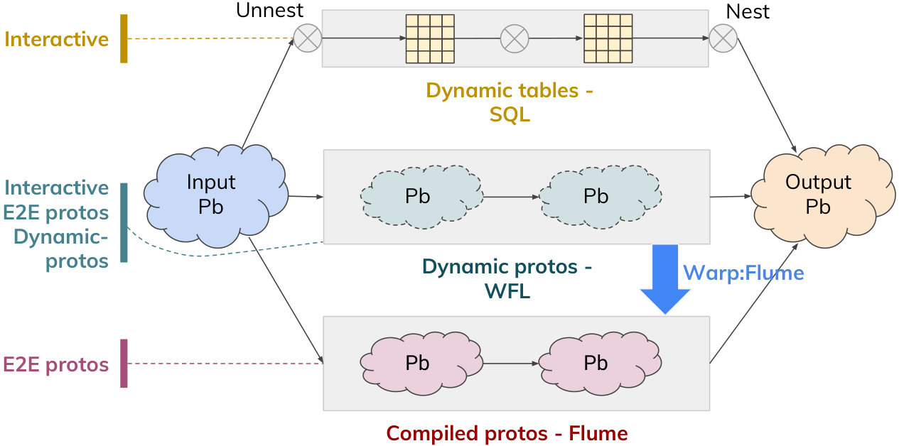 Figure 1
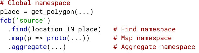 Figure 2
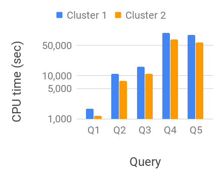 Figure 3
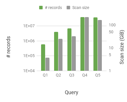 Figure 4
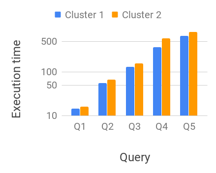 Figure 5
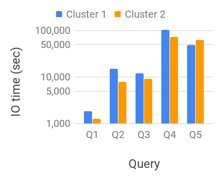 Figure 6
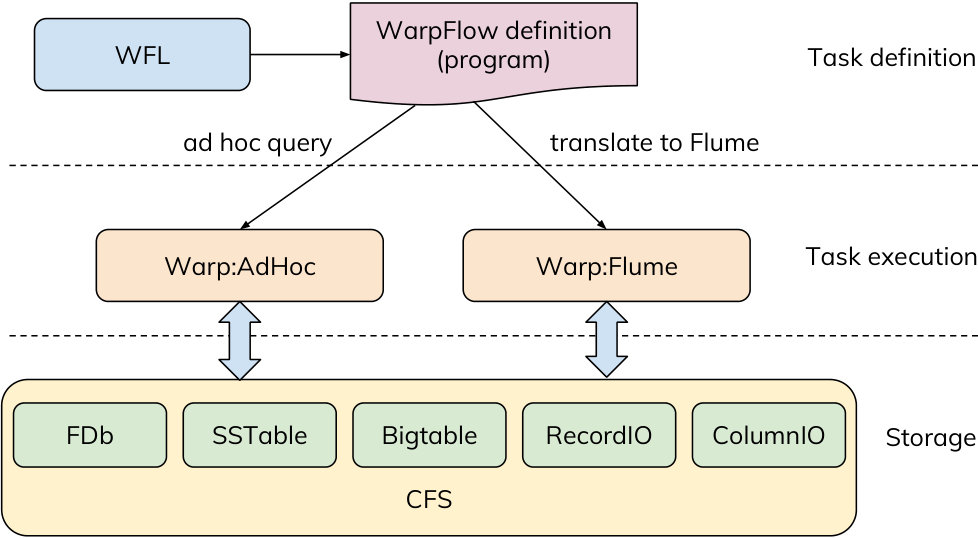 Figure 7
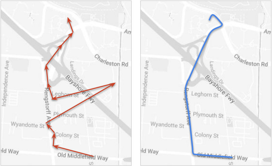 Figure 8
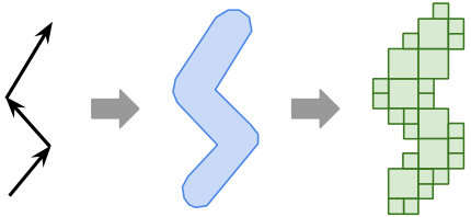 Figure 9
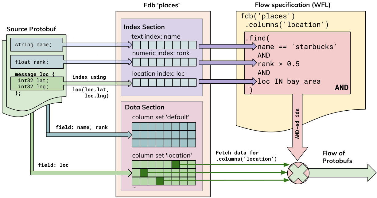 Figure 10
 Figure 11
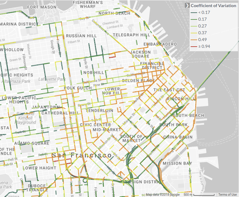 Figure 12
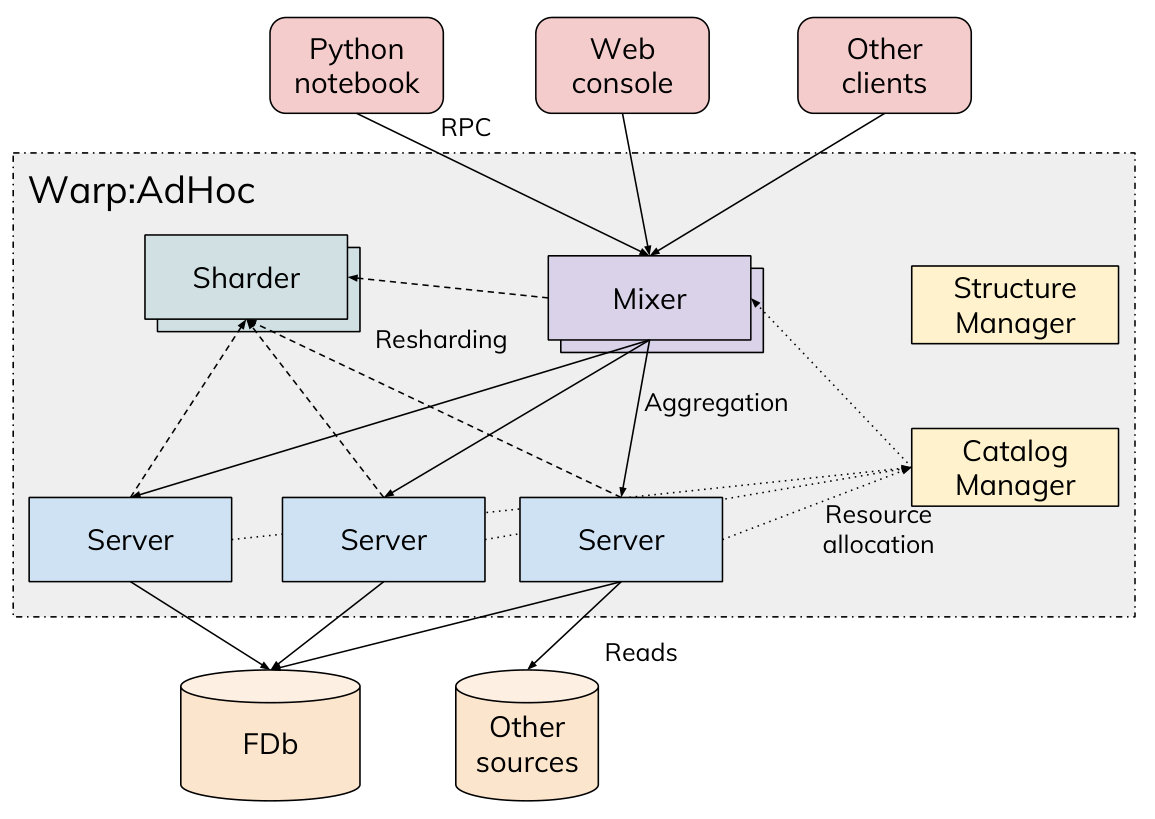 Figure 13
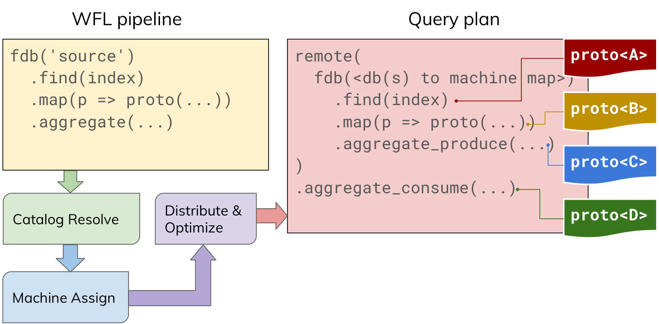 Figure 14
| Operator | Function |
|---|---|
| Basic transformations | |
| map | Transform a Protocol Buffers record into another Protocol Buffers record. |
| filter | Filter records in the flow based on boolean condition. |
| flatten | Flatten repeated fields within Protocol Buffers into multiple Protocol Buffers. |
| Reordering a flow | |
| sort_asc, sort_desc | Sort the flow (in ascending or descending order) using an expression. |
| Resizing a flow | |
| limit | Limit the number of records in the flow. |
| distinct | Remove duplicate records from the flow, based on an expression. |
| aggregate | Aggregate the records in the flow, possibly grouping them by one or more fields or expressions, using predefined aggregates (e.g., count, sum, avg). |
| Merging flows | |
| join | Merge Protocol Buffers from two different flows using a hash join. |
| sub_flow | Join Protocol Buffers from the flow with a sub-flow using index join. |
| Materializing a flow | |
| collect | Collect the Protocol Buffers records from the flow into a variable. |
| save, to_sstable, to_recordio | Saves the Protocol Buffers from the flow to FDb, SSTable or RecordIO (mis, 2014). |
| Query | CPU time | Exec. time |
|---|---|---|
| Geospatial index | 5.4 h | 2.2 m |
| Multiple indices | 45 m | 17.6 s |
| 10% sample | 4 m | 12.0 s |
| 1% sample | 23 s | 11.2 s |
Peer Reviews
No public reviews on file for this paper yet. If you reviewed it on a platform where reviews are public (OpenReview, ICLR, NeurIPS, ICML), you can paste yours below so the community can read it here.
Videos
No videos yet. Explain this paper in a talk, walkthrough, or lecture? Add one.
Taxonomy
TopicsData Management and Algorithms · Human Mobility and Location-Based Analysis · Geographic Information Systems Studies
WarpFlow: Exploring Petabytes of Space-Time Data
Catalin Popescu
Google, Inc.
,
Deepak Merugu
Google, Inc.
,
Giao Nguyen
Google, Inc.
and
Shiva Shivakumar
Google, Inc.
Abstract.
WarpFlow is a fast, interactive data querying and processing system with a focus on petabyte-scale spatiotemporal datasets and Tesseract queries. With the rapid growth in smartphones and mobile navigation services, we now have an opportunity to radically improve urban mobility and reduce friction in how people and packages move globally every minute-mile, with data. WarpFlow speeds up three key metrics for data engineers working on such datasets – time-to-first-result, time-to-full-scale-result, and time-to-trained-model for machine learning.
1. Introduction
Analytical data processing plays a central role in product development, and designing and validating new products and features. Over the past few years, we have seen a surge in demand for petascale interactive analytical query engines (e.g., Dremel (Melnik et al., 2010), F1 (et al., 2013), Shasta (et al., 2016)), where developers execute a series of SQL queries over datasets for iterative data exploration. Also, we have seen a tremendous growth in petascale batch pipeline systems (e.g., MapReduce (Dean and Ghemawat, 2008), Flume (et al., 2010), Spark (Zaharia et al., 2010)), where developers express map-reduce and parallel-do style processing over datasets in batch mode.
In this paper, we focus on an important query pattern of ad hoc Tesseract111In geometry, Tesseract is the four-dimensional analog of a cube. It is popularized as a spatiotemporal hyper-cube in the film Interstellar, and as the cosmic cube containing the Space Stone with unlimited energy in the Avengers film series. queries. These are“big multi-dimensional joins” on spatiotemporal datasets, such as datasets from Google Maps, and the fast-growing passenger ride-sharing, package delivery and logistics services (e.g., Uber, Lyft, Didi, Grab, FedEx). For example, a billion people around the world use Google Maps for its navigation and traffic speed services (mis, 2018e), finding their way along 1 billion kilometers each day (mis, 2017a). To constantly improve the service on every minute-mile, engineers answer questions such as: (1) which roads have high speed variability and how many drivers are affected, (2) how many commuters, in aggregate, have many travel modes, e.g., bike after taking public transit? (3) what are restaurant wait times when they are busy?
For such queries, we need to address a few important challenges:
- •
How to analyze large, and often noisy spatiotemporal datasets? Most of this data comes from billions of smartphones moving through urban environments. These devices compute current location estimate by fusing GPS, WiFi, cellular signal and other available sensors, with varying degrees of accuracy (often 3 – 30 meters away from the true position), based on urban canyon effects, weather and indoor obstructions (Zandbergen and Barbeau, 2011; Lee et al., 2016; von Watzdorf and Michahelles, 2010). These location observations are then recorded on the device and pushed to the cloud with an accuracy estimate. Also, each navigation path is recorded as a time-series of such noisy observations. A few key questions include: (a) how to store and index such rich data (e.g., locations and navigation paths), (b) how to address noise with filtering and indexing techniques?
- •
How to speedup developer workflow while iterating on such queries? Each typical developer workflow begins with a new idea. The developer then tests the idea by querying the datasets, usually with simplified queries on small samples of the data. If the idea shows promise, they validate it with a full-scale query on all the available data. Depending on the outcome, they may repeat these steps several times to refine or discard the original idea. Finally, the developer pushes the refined idea towards production.
One hurdle in this development cycle is the lengthy iteration time – long cycles (several hours to days) prevent a lot of potential ideas from being tested and refined. This friction arises from: (i) long commit-build-deploy cycles when using compiled pipelines, and (ii) composing complex queries on deeply nested, rich data structures (e.g., Protocol Buffers (mis, 2017b), an efficient binary-encoded, open-source data format widely used in the industry). To improve developer productivity, it is important to speed up the time-to-first-result, time-to-full-scale-result, and time-to-trained-model for machine learning. On the other hand, from a distributed systems standpoint, it is hard to simultaneously optimize for pipeline speed, resource cost, and reliability.
- •
How do we make a production cluster, hosting several large datasets with multiple developers simultaneously running pipelines, cost efficient by reducing the resource footprint? This is a common problem especially for developers in popular clusters (e.g., AWS, Azure, Google Cloud) who scale up (or down) their clusters for analytic workloads, because it is inefficient to dedicate a full cluster of machines and local storage. For example, consider a 20 TB dataset. We could use a dedicated cluster with 20 TB of RAM and local storage to fit the entire data in memory. However, it is about 5 cheaper if we use a system with 2 TB of RAM, and about 40 cheaper if we use a system with 200 GB of RAM coupled with network storage (mis, 2018a). Moreover, the operational overhead with building and maintaining larger clusters is magnified as the memory requirements increase for petabyte scale datasets. As we see later, our system is built with these constraints in mind and offers good performance while being cost efficient.
In this paper, we discuss how WarpFlow addresses such challenges with below features:
- •
Supports fast, interactive data analytics to explore large, noisy spatiotemporal datasets with a pipeline-based query language using composite indices and spatiotemporal operators. The underlying techniques are easy to deploy in a cost-efficient manner on shared analytics clusters with datasets available on networked file systems such as in AWS, Microsoft Azure, Google Cloud (mis, 2018a, f, d).
- •
Supports two complementary execution modes – (i) an “insane” interactive mode, with an always-on speed optimized cluster and “best effort” machine failure tolerance, and (ii) a batch mode for running large-scale queries with auto-scaling of resources and auto-recovery for reliable executions. In batch mode, WarpFlow automatically generates an equivalent Flume pipeline and executes it. In practice, we see development times are often 5 – 10 faster than writing and building equivalent Flume pipelines from scratch, and helps our data developers gain a big productivity boost.
- •
Accelerates machine learning workflows by providing interfaces for faster data selection and built-in utilities to generate and process the training and test data, and enabling large-scale model application and inference.
The rest of the paper is structured as follows. In Section 2, we present related work and contrast our goals and assumptions. In Section 3, we give an overview of WarpFlow and its design choices. The detailed architecture of WarpFlow and its components is presented in Section 4. We present the application of WarpFlow to machine learning use cases in Section 5. We present an example use case and experimental results in Section 6, followed by conclusions in Section 7.
2. Related Work
WarpFlow builds on years of prior work in relational and big data systems, spatiotemporal data and indexing structures. In this section, we will summarize the key common threads and differences. To the best of our knowledge, this is the first system (and public description) that scales in practice for hundreds of terabytes to petabytes of rapidly growing spatiotemporal datasets. While there are large spatial image databases that store petabytes of raster images of the earth and the universe (e.g., Google Earth), they of course have different challenges (e.g., storing large hi-resolution images, and extracting signals).
First, systems such as PostgreSQL (mis, 2018i), MySQL (mis, 2018g) offer a host of geospatial extensions (e.g., PostGIS (mis, 2018h)). To tackle larger datasets on distributed clusters, recent analytical systems propose novel extensions and specialized in-memory data structures (e.g., for paths and trajectories) on Spark/Hadoop (Zaharia et al., 2010) clusters (Eldawy, 2014; Xie et al., 2016, 2017; Shang et al., 2018; Costa et al., 2017; Yu et al., 2015).
Specifically, the techniques in (Xie et al., 2016, 2017; Shang et al., 2018) adopt Spark’s RDD model (Zaharia et al., 2010) and extend it with a two-level indexing structure. This helps prune RDD partitions but partitions containing matched data need to be paged into memory for further filtering. These techniques work well when (1) the data partition and indices fit in main memory on a distributed cluster, (2) data overflows are paged into local disks on the cluster, (3) the queries rely on the partition and block indices to retrieve only relevant data partitions into available memory. In such cases, the techniques work well to optimize CPU costs and can safely ignore IO costs in a cluster. However, for our pipelines, we deal with numerous large datasets on a shared cluster, so developers can run pipelines on these datasets concurrently. We need to optimize both CPU and IO costs making use of fine-grained indexing to selectively access the relevant data records, without first having to load the partitions. As we see later, our techniques scale for multiple, large datasets on networked file systems, while minimizing the resource footprint for cost efficiency.
Second, WarpFlow supports two execution environments for pipelines. For long running pipelines that need to deal with machine restarts and pipeline retries, systems like MapReduce (Dean and Ghemawat, 2008), Flume (et al., 2010) and Spark (Zaharia et al., 2010) adopt checkpoint logs that allow a system to recover from any state. For fast, interactive and short-running queries, systems like Dremel (Melnik et al., 2010) drop this overhead, support an always running cluster and push retries to the client applications. WarpFlow supports the best of both worlds, by offering the developer two modes by relying on two separate execution engines – one for long running queries and one for fast, interactive queries.
Third, how to express complex transformations on rich data has been an area of active work, from SQL-like declarative formats to full procedural languages (e.g., Scala, C++). For example, Shasta (et al., 2016) uses RVL, a SQL-like declarative language to simplify the queries. In contrast, WarpFlow’s language (WFL) uses a functional query language to express rich data transformations from filters, aggregates, etc. to machine learning on tensors. To speed up the iterations, WFL does not have a compilation step and interprets the query dynamically at runtime. In addition, WFL is extensible to natively support external C++ libraries such as TensorFlow (mis, 2018k). This makes it easy to integrate domain-specific functionalities for new types of large-scale data analysis. Using a common WarpFlow runtime for data-intensive operations speeds up the overall process, similar to Weld (Palkar et al., 2016). However, Weld integrates multiple libraries without changing their APIs by using an optimized runtime, while WarpFlow provides a compatible API to use libraries and their functions. Like F1 (et al., 2013), WarpFlow uses Protocol Buffers as first-class types, making it easy to support rich, hierarchical data. Furthermore, WarpFlow uses Dynamic Protocol Buffers (mis, 2017c), so that developers can define and consume custom data structures on the fly within the query. As we see later, this helps developers to iterate on pipelines without expensive build-compile cycles.
3. Overview
A WarpFlow pipeline consists of a data source that generates the flow of Protocol Buffers, followed by operators that transform the Protocol Buffers, and the expressions to define these transformations. WarpFlow is fully responsible for maintaining the state of the datasets including data sharding and placement, distributing the pipeline, executing it across a large cluster of machines, and load-balancing across multiple concurrent queries.
For example, consider how to evaluate the quality of a road speed prediction model. To get a quick insight, we look at the routing requests in San Francisco in the morning rush hour from 8 am – 9 am. We start with the roads dataset – a collection of roads along with their identifiers and geometry, and use its indices to generate a stream of Protocol Buffers corresponding to roads in San Francisco. For each road segment, we apply our speed prediction model to get the predicted speed for 8 am – 9 am, and compute the distance of the road segment from its polyline. Next, we use the route requests dataset, which is a collection of all routing requests along with the request time, the suggested route and the actual travel time, and use its indices to get all relevant route requests. We join the results with the road segment information from the previous step, and use the distance and the predicted speed of the road segments along the suggested route to compute the predicted travel time. The difference in the predicted travel time and the actual travel time gives the error in our prediction. Finally, we aggregate these measurements to get the mean and standard deviation of the errors in travel time.
WarpFlow facilitates such common operations with a concise, functional programming model. Figure 1 shows a WFL snippet for the previous example; the red fields are repeated (vectors) and the pink fields are TensorFlow objects. Notice (1) index-based selections to selectively read only the relevant records, and (2) operators for vectors, TensorFlow model applications, and geospatial utilities. For example, the dictionary lookups using a vector to get the road segments, the vector division to get travel times per segment, and the geospatial utility for distance computation.
3.1. Design choices
Consider how to query and transform a Protocol Buffers dataset into a new Protocol Buffers result set. Figure 2 presents a simplified conceptual depiction of different data processing systems, along with some of the relevant benefits they offer (e.g., interactivity, end-to-end Protocol Buffers, Dynamic Protocol Buffers, etc.).
Data pipeline model
Data is usually modeled as relational or hierarchical structures. Systems either: (a) retain Protocol Buffers and manipulate them directly (e.g., MapReduce, Flume, Spark), or (b) re-model data into relational tables (e.g., flatten repeated fields) and manipulate with relational algebra (e.g., MySQL, Dremel, F1).
WarpFlow chooses (a): it retains Protocol Buffers at every stage of the pipeline, for inputs, transforms, and outputs. Similar to Flume and Spark, developers compose deep pipelines of maps, filters, and aggregates on these hierarchical and nested structures.
Interactivity
Interactivity is a highly desirable feature for developers, often termed as REPL (read-evaluate-print-loop) in popular frameworks like Python and Scala (mis, 2018j). Interactive data systems enable developers to quickly compose/iterate and run queries, reducing the time-to-first-result and speeding up the development and debug cycle with instant feedback. Such systems are typically interpreted in nature as opposed to being compiled, and have short runtimes to execute full and incremental queries in a session.
WarpFlow offers a similar experience by making it easy for developers to (a) access and operate on the data, and (b) iteratively build pipelines. Specifically, it supports:
- •
Always-on cluster for distributed execution of multiple ad hoc queries in parallel. Composite indices over hierarchical datasets and popular distributed join strategies (Garcia-Molina et al., 2008) to help developers fine-tune queries, such as broadcast joins, hash joins and index-based joins.
- •
Query sessions to incrementally build and run queries with partial context kept in the cluster while the user refines the query. Also, full auto-complete support in query interfaces, not just for the language but also for the structure of the data, and the data values themselves.
- •
A strong toolkit of spatiotemporal functions to work with rich space-time datasets, and utilities to allow querying over a sample to quickly slice through huge datasets.
4. Architecture
The WarpFlow system has three key components to handle the data storage, task execution, and task definition functionalities, as shown in Figure 3. The data storage layer holds the Protocol Buffers data sources in one of several common storage formats. In addition, WarpFlow builds custom “FDb” indices, optimized for indexing Protocol Buffers data. The task execution layer reads the Protocol Buffers data from the storage layer and carries out the query execution. WarpFlow supports two execution modes. The pipelines run in an interactive, ad hoc manner using “Warp:AdHoc”, or as a batch job on Flume using “Warp:Flume”. The specification of the query and its translation to the execution workflow is carried out by the task definition layer. WarpFlow uses a functional query language, called “WarpFlow Language” (WFL), to express the queries concisely.
In this section, we describe each of the key components in detail.
4.1. Data storage and indexing
In the following sections, we describe the underlying structure and layout of FDb, and the different index types that are available.
4.1.1. FDb: Indexing and storage format
FDb is a column-first storage and search database for Protocol Buffers data. Like many distributed data formats, FDb is a sharded storage format, sharding both the data and the indices. Each FDb shard stores data values organized by column sets (similar to column families in Bigtable (Chang et al., 2008)) and index values mapped to document-ids within the shard.
The basic FDb layout is illustrated in Figure 4 showing a sample Protocol Buffers record with fields name, rank and a sub-message loc with fields lat and lng. The data layout has separate sections for indices and data. The data section is further partitioned into column sets. A sample query, shown on the right in Figure 4, accesses the necessary indices to narrow down the set of documents to read, which are then read column-wise from the column sets.
FDb is built on a simple key-value storage abstraction and can be implemented on any storage infrastructure that supports key-value based storage and lookups e.g., LevelDb (mis, 2011), SSTable (Chang et al., 2008), Bigtable, and in-memory datastores. We use SSTables to store and serve our ingested datasets as read-only FDbs. The sorted key property is used to guarantee iteration-order during full table scans and lookups. We implement read-write FDbs on Bigtable for streaming FDbs, including for query profiling and data ingestion logs.
4.1.2. Index types
FDb supports indexing a variety of complex value types. A single field in the Protocol Buffers (e.g., navigation path) can have multiple indices of different types. In addition to basic inverted text and range indices for text and numeric values, FDb supports geometry based indices e.g., locations, areas, segments, etc. as described below.
location
Location indices are intended for data fields that represent punctual places on the Earth, typically identified by latitude and longitude. Internally, we use an integer-representation of the location’s Mercator projection (Maling, 2013) with a precision of several centimeters. As such, locations to the north of N and south of S are not indexable without some translation. The selection of location index can be specified by a bounding box (with south-west and north-east corners) or by a region (e.g., a polygonal area) to fetch all the documents where the location field is within the given region.
area
Area index is used for geospatial regions, usually represented by one or more polygons. We use area trees to represent these indices. The selection of areas can be made efficiently, either by a set of points (i.e., all areas that cover these points) or by a region (i.e., all areas that intersect this region). In addition, these indices are also used to index geometries other than regions by converting them to representative areas. For example, a point is converted to an area by expanding it into a circular region of a given radius; a path is converted to an area by expanding it into a strip of a given width. These areas are then indexed using an area tree, as shown in Figure 5. This enables indexing richer geospatial features such as navigation paths, parking and event zones.
Area trees are very similar to quad-trees (Finkel and Bentley, 1974); the main difference is that the space of each node is split into 64 () sub-nodes as opposed to four () sub-nodes in a quad-tree. The 64-way split of each node leads to an efficient implementation and maps naturally to the gridding of the Earth in the spherical Mercator projection. They can be combined (union, difference or intersection) in a fast, efficient manner, and can be made as fine as needed for the desired granularity (a single pixel can represent up to a couple of meters). In addition to indexing purposes, they are used for representing and processing geospatial areas in a query.
Indices and column sets are annotated on the Protocol Buffers specification using field options. For any field or sub-field in the message, we use options to annotate it with the index type (e.g., options index_text and index_tag to create text and tag indices). We also define the mapping of fields to column sets. In addition, we can define virtual fields for the purpose of indexing. These extra fields are not materialized and are only used to create the index structure.
4.1.3. Data de-noising
As mentioned earlier, spatiotemporal data from devices often have poor location accuracy or occasional bad network links. Our pipelines need to be resilient to noisy data, and should filter and smooth the data. The presence of noise transforms a precise location or a path into a probabilistic structure indicating the likely location or path. WarpFlow provides methods to construct and work with probabilistic representations of the spatial data, and to project and snap them to a well-defined space. For example, we can snap a noisy location to a known point-of-interest (POI), or snap a noisy navigation path with jittered waypoints to a smooth route along road segments, as shown in Figure 6. Snapping is often done by selecting the fuzzy regions of interest and applying a machine-learned (ML) model using signals such as the popularity of places and roads, similarity to other crowdsourced data, and suggested routes from a routing engine (as we see later, WarpFlow supports TensorFlow to train and apply ML models).
Area indices help us work with such noisy geospatial data and snappings. Representative areas are a natural way to identify probabilistic locations and paths. For example, a probabilistic location can be represented by a mean location and a confidence radius (i.e., a circular region) depending on the strength of the noise. Similarly, a probabilistic path can be represented by a curvilinear strip whose thickness indicates the strength of the noise. Recall that this area is not a bounding box of the points in a path, but an envelope around the path so time ordering is preserved. We can then use this fuzzy selection of data and intersect with filter conditions. As we see later, these simple, fuzzy selections help us handle large datasets in a cost-efficient fashion on shared cloud clusters.
4.2. WarpFlow language (WFL)
WarpFlow uses a custom, functional programming language, called WarpFlow language (WFL), to define query pipelines with hierarchical datasets. A common problem when working with deeply nested, hierarchical data structures (e.g., Protocol Buffers) is how to (1) first express the query pipelines, and (2) later, evolve the pipelines as underlying structures and requirements change. To address this problem, WFL draws inspiration from modern, functional languages, such as Scala (mis, 2018n) that draw on decades of software engineering best practices for code structuring, maintenance, and evolution. WFL adopts two key elements for succinct queries: (1) a pipeline-based approach to transform data with sequentially chained operations, and (2) hierarchical structures as primitive data types, so operators work on vectors, tensors and geospatial structures.
The full language definition and its constructs are out of the scope of this paper. Instead, we present a simplified overview of the language in this section.
4.2.1. Data types
Protocol Buffers objects in WFL have two properties: (1) type: the data type of the object, which is one of {bool, int, uint, float, double, string, message}. (2) cardinality: the multiplicity of the object i.e., singular or repeated; singular and repeated fields are treated as scalars and vectors respectively for most operations.
In addition to the basic data types, WFL provides utilities such as array, set, dict and geo-utilities (e.g., point, area, polygon, etc.) to compose basic data types into pre-defined, higher-level objects.
4.2.2. Operators and expressions
Each stage in a WFL pipeline generates a series of Protocol Buffers records with the same structure. We call this series a flow of Protocol Buffers. Flow provides operators that transform the underlying Protocol Buffers. Most of these operators accept a function expression as an argument, that defines the transformation to be performed. Each operator, in turn, generates a new flow of transformed Protocol Buffers. A typical WFL pipeline with several chained operators has the following syntax:
flow .<flow_operator_1>(p => {body_1}) .<flow_operator_2>(p => {body_2}) .<flow_operator_3>(p => {body_3})
A transformation is defined using expressions composed of the aforementioned data types, operators, and higher-order functions, like in any programming language. The expression body does not have a return statement; the final statement in the body becomes its return value. Each flow operator may require a specific return type, e.g., a filter operator expects a boolean return type and a map operator expects a Protocol Buffers return type. The primary flow operators and their functions are presented in Table 1.
Expressions compose data types using simple operators, e.g., +, -, *, /, %, AND, OR, IN, BETWEEN. These operators are overloaded to perform the corresponding operation depending on the type of the operands. In addition to these simple operators, a collection of utilities make it easier to define the transformations.
Furthermore, WFL seamlessly extends the support for these operations to repeated data types. If one or more of the operands is of a repeated data type, the operation is extended to every single element within the operand. This greatly simplifies the expressions when working with vectors, without having to iterate over them.
Finally, WFL offers a large collection of utilities to simplify and help with common data analysis tasks. Besides basic toolkits to work with strings, dates and timestamps, it provides advanced structures such as HyperLogLog sketches for cardinality estimation of big data (Flajolet et al., 2007), Bloom filters (Bloom, 1970) for membership tests, and interval trees (Cormen et al., 2009) for windowing queries. It also has a geospatial toolkit for common operations such as geocoding, reverse-geocoding, address resolution, distance estimation, projections, routing, etc.
4.2.3. Extensibility
In addition to the built-in features and functions, WFL is designed to be an extensible language. It allows custom function definitions within WFL. It also features a modular function namespace for loading predefined WFL modules. Furthermore, we can easily extend the language by wrapping the APIs for third-party C++ libraries and exposing them through WFL. We use this approach to extend WFL to support TensorFlow (mis, 2018k) API, enabling machine learning workflows with big data (see Section 5 for more details). This capability elevates the scope of WarpFlow by providing access to the vast body of third-party work.
4.3. WarpFlow execution
WarpFlow pipelines can be executed as interactive, ad hoc jobs with Warp:AdHoc, or as offline, batch jobs with Warp:Flume depending on the execution requirements. Developers typically use Warp:AdHoc for initial data explorations and quick feedback on sampled datasets. The same WFL pipeline can later be executed on full-scale datasets as a batch job on Flume using Warp:Flume. In this section, we first describe Warp:AdHoc and its underlying components. The logical model of data processing is maintained when converting WFL pipelines to Flume jobs using Warp:Flume.
4.3.1. Warp:AdHoc
Warp:AdHoc is an interactive execution system for WFL pipelines. A query specification from WFL is translated into a directed acyclic graph (DAG) representing the sequence of operations and the flow of Protocol Buffers objects from one stage to the next. Warp:AdHoc performs some basic optimizations and rewrites to produce an optimized DAG. The execution system is responsible for running the job as specified by this DAG.
The high-level architecture of Warp:AdHoc is shown in Figure 7. Developers work on clients such as an interactive Python notebook (e.g., Jupyter (mis, 2018m), Colaboratory (mis, 2018c)), or a web-based console, which interact with Warp:AdHoc via a remote interface. Through this interface, clients communicate with a Mixer, which coordinates query execution, accumulates and returns the results. The Mixer distributes the execution to Servers and Sharders depending on the query.
The system state of Warp:AdHoc is maintained by a few metadata managers. Specifically, Structure manager maintains a global repository of Protocol Buffers structures defined statically or registered at run-time. Catalog manager maintains pointers to all registered FDbs, and maps them to Servers for query and load distribution.
4.3.2. Dataset structures
Although Warp:AdHoc can read and transform data from a variety of sources, queries executed over them are typically slower due to full-scan of data. FDb is the preferred input data source for Warp:AdHoc, where indices over one or more columns can be used in find() to only read relevant data.
Warp:AdHoc needs to know the structure of the Protocol Buffers representing the underlying data. For non-FDb data sources, these are provided by the developer. For FDb sources these structures are typically registered using the name of the Protocol Buffers with the Structure manager, and are referred to directly by these names in WFL pipelines. These structures can be added, updated, or deleted from the Structure manager as necessary.
4.3.3. Dynamic Protocol Buffers
SQL-based systems like Dremel and F1 enable fast, interactive REPL analysis by supporting dynamic tables. Each SQL SELECT clause creates a new table type, and multiple SELECTs can be combined into arbitrarily complex queries. However, users do not need to define schemas for all these tables – they are created dynamically by the system.
Similarly, WarpFlow uses Dynamic Protocol Buffers (mis, 2017c) to provide REPL analysis. WFL pipelines define multi-step data transformations, and the Protocol Buffers schema for each stage is created dynamically by the system using Dynamic Protocol Buffers.
For instance, in the sample WFL pipeline in Figure 8, the output of each stage (e.g., map, aggregate) has a Protocol Buffers structure that is different from that of the source, and the necessary Protocol Buffers schemas are implicitly defined by the system.
In addition, a WFL pipeline has a global namespace and a tree of local namespaces corresponding to pipeline stages and functions. Each namespace has variables with static types inferred from assignments. Values in these namespaces can be used in Protocol Buffers transformations, as shown in the find() clause in Figure 8. These namespaces are also represented by Dynamic Protocol Buffers with fields corresponding to their defined variables.
In a relational data model, the data is usually normalized across multiple tables with foreign-key relationships, reducing the schema size of an individual table. In hierarchical datasets, the entire nested data is typically stored together. Sometimes, the structure of this data has a deep hierarchy that recursively loads additional structures, resulting in a schema tree with a few million nodes. Loading the entire schema tree to read a few fields in the source data is not only redundant but also has performance implications for interactive features (e.g., autocompletion).
Instead, WarpFlow generates the minimal viable schema by pruning the original Protocol Buffers structure tree to the smallest set of nodes needed for the query at hand (e.g., tens of nodes as opposed to millions of nodes). It then composes a new Dynamic Protocol Buffers structure with the minimal viable schema which is used to read the source data. This reduces the complexity of reading the source data and improves the performance of interactive features.
4.3.4. Query planning
When a WFL query is submitted to Warp:AdHoc, a query plan is formulated to determine pipeline distribution and resource requirements, similar to distributed database query optimizers (Garcia-Molina et al., 2008). Most stages in the pipeline are executed remotely on the Servers, followed by an optional final aggregation on the Mixer. Query planning involves determining stages of the pipeline that are remotely executed, the actual shards of the original data source that are required for the query, and the assignment of execution machines to these shards. Depending on the query, the planning phase also optimizes certain aspects of the execution. For example, a query involving an aggregation by a data sharding key is fully executed remotely without the need for a final aggregation on the Mixer.
Query planning also determines the Protocol Buffers structures at different stages in the pipeline. The structures for parts of the query that are executed remotely are distributed to the respective Servers and Sharders.
The query plan for a typical WFL query is shown in Figure 9. The pipelines within remote(...) execute on individual Servers reading data from the assigned FDb shards from a common file system. The aggregate_consume(...) stage aggregates partial results received from all the remote pipelines on the Mixer.
Data is transformed through different Protocol Buffers structures as it passes through different stages in the pipelines. For example, in Figure 9, proto<A> is the structure of the FDb source data while proto<B>, proto<C> and proto<D> are the structures of the output of map(), aggregate_produce() and aggregate_consume() stages respectively.
4.3.5. Distributed execution
Warp:AdHoc executes WFL pipelines using a distributed cluster of Servers and Sharders. Each WFL query requires the necessary resources (execution servers) to be allocated before its execution begins. These resources are requested from the Catalog manager, after the query planning phase. If resources are not immediately available then the query waits in a queue until they are allocated. Eventually, the Catalog manager allocates the Servers for execution, along with assigning a subset of FDb shards to each Server for local reads and transformations.
The query execution starts by setting up the corresponding pipeline stages on Servers, Sharders and the Mixer. Servers then start reading from their assigned FDb shards, transform the data as necessary, and return partial results to the Mixer. Sharders perform intermediate shuffles and joins as specified by the pipeline. The Mixer pipeline aggregates the partial results and returns the final results to the client. To reclaim the resources when a query is blocked, a time limit is imposed at various stages and its execution is re-attempted or aborted.
WarpFlow makes it easy to query enormous amounts of data, for concurrent queries. It offers execution isolation – each query gets its own dedicated micro-cluster of Servers and Sharders for the duration of its execution. This ensures that queries do not interfere with each other.
4.3.6. Warp:Flume
In addition to interactive execution, WarpFlow can automatically translate WFL queries to Flume jobs for large-scale, batch processing. Warp:Flume is the component of WarpFlow that is responsible for this translation and execution.
Each stage of a WFL pipeline is internally implemented using processors, such as find processor for find(), map processor for map(), and so on. To enable the translation to Flume jobs, each processor is wrapped into a Flume function. In addition to these processors, we also implement specialized Flume data readers that can work with FDb data sources and use index selection for data fetching. The data processed by a pipeline stage is wrapped into standard Flume data types such as flume::PCollection and flume::PTable<K,V> (et al., 2010), depending on the type of the processor.
Warp:AdHoc uses Dynamic Protocol Buffers to pass data between the stages. For Warp:Flume, we use two ways to pass the data between the stages: (i) String encoding – convert all the Protocol Buffers to strings, pass the string data to the next stage, which then deserializes them into Protocol Buffers; (ii) Protocol Buffers encoding – we retain the data as Protocol Buffers and share the pointers between the stages, along with custom coders to process these Dynamic Protocol Buffers. From our experiments, we notice that option (i) tends to be faster for simple pipelines with few stages where the encoding and decoding overhead is minimal, but option (ii) is faster for longer pipelines with heavy processing and multiple stages. In general, we notice a 25% performance penalty when compared with an equivalent, hand-written Flume job. Nevertheless, with Warp:Flume we typically see development times are faster by about 5 – 10. We believe the speed up in the development time more than compensates for the small overhead in runtimes.
5. Machine learning
Machine learning (ML) brings novel ways to solve complex, hard-to-model problems. With WarpFlow’s extensible data pipeline model, we support TensorFlow (mis, 2018k) as another pipeline operator extension for common use cases. A typical workflow of an ML developer has the following main steps:
- (1)
Design a prototype ML model with an input feature set to provide an output (e.g., estimations or classifications) towards solving a problem. 2. (2)
Collect labeled training, validation, and test data. 3. (3)
Train the model, validate and evaluate it. 4. (4)
Use the saved model to run large-scale inference or a large-scale evaluation.
Usually, steps 1 – 3 are repeated in the process of iterative model refinement and development. A lot of developer time is spent in feature engineering and refining the model so it is best able to produce the desired outputs. Each iteration involves fetching training, validation and test data that make up these features. In some cases, we see wait times of a few hours just to extract such data from large datasets.
Quick turn around times in these steps accelerate the development and enable testing richer feature combinations. Towards this end, WFL is extended to natively support TensorFlow APIs for operations related to basic tensor processing, model loading and model inferences.
To be able to fetch the data and extract the features from it, a set of basic tensor processing operations are provided through TensorFlow utilities in WFL. This minimal set of operations enables basic tensor processing and marshaling that is needed to compose and generate features from a WFL query.
After getting hold of the data and the features, the training is performed independently, usually in Python. While training within WarpFlow is possible, it is often convenient to use frameworks that are specifically designed for accelerated distributed training on specialized hardware (mis, 2018b). WarpFlow helps the developers get to the training faster through easy data extraction.
With the completion of the training phase, there are the following use cases for model application:
- •
Trained models are typically evaluated on small test datasets, after the training cycle. However, the model’s performance often needs to be evaluated on much bigger subsets of the data to understand the limitations that might be helpful in a future iteration.
- •
Once a model’s performance has been reasonably tested, the model can be used for its inference – predictions or estimations of the desired quantities. A common use case is to run the model offline on a large dataset and annotate it with the inferences produced by the model. For example, a model trained to identify traffic patterns on roads can be applied offline on all the roads and annotate their profile with predicted traffic patterns; this can later be used for real-time traffic predictions and rerouting.
- •
As an alternative to offline application, the inferences of the model can be used in a subsequent query that is computing derived estimates i.e., the model is applied online and its inferences are fed to the query.
To enable the above use cases, a set of TensorFlow utilities related to model loading and application are added to WFL. For easier interoperability with other systems, these utilities are made compatible with the standard SavedModel API (mis, 2018l).
6. Experiments
A billion people around the world use Google Maps for its navigation and traffic speed services, finding their way along 1 billion kilometers each day. As part of this, engineers are constantly refining signals for routing and traffic speed models. Consider one such ad hoc query: “Which roads have highly variable traffic speeds during weekday mornings?” In this section, we evaluate the performance of WarpFlow under different criteria for such queries.
For this paper, we use the following dataset and experimental setup to highlight a few tradeoffs.
- •
Google Maps maintains a large dataset of road segments along with their features and geometry, for most parts of the world. It also records traffic speed observations on these road segments and maintains a time series of the speeds. For these experiments, we use only the relevant subset of columns (observations and speeds) for past 6 months ( 27 TB). For this dataset, we want to accumulate all the speed observations per road segment during the morning rush hours (8 – 9 am on weekdays), and compute the standard deviation of the speeds, normalized with respect to its mean – we call this the coefficient of variation.
- •
We setup a Warp:AdHoc execution environment on two different micro-clusters: (1) Cluster 1 with 300 servers with a total equivalent of 965 cores of Intel Haswell Xeon (2.3GHz) processors and 3.5 TB of RAM, and (2) Cluster 2 with 110 servers with a total equivalent of 118 cores and 330 GB of RAM. Note that these clusters have about 13% and 1.2% RAM respectively relative to the dataset size, and cost about 5 and 40 lower when compared to a cluster with 100% RAM capacity as required by other main-memory based techniques discussed in Section 2.
We run below series of queries on this dataset to compute traffic speed variations over different geospatial and time regions. Then to visualize the speed variations on roads for query Q1, we join the resulting data with the dataset of road geometry and render them on a map. For example, Figure 10 shows the variations for roads in San Francisco.
- •
Q1: San Francisco over a month
- •
Q2: San Francisco over 6 months
- •
Q3: San Francisco Bay Area (including Berkeley, South Bay, Fremont, etc.) over a month
- •
Q4: San Francisco Bay Area over 6 months
- •
Q5: California over a month
In addition, we run these queries with different selection criteria, described below. Table 2 shows the total CPU time and the execution time for Q1 on Cluster 1.
Geospatial index
Instead of scanning all the records and filtering them, we use the geospatial indices to only select relevant road segments and filter out observations that are outside the morning rush hours on weekdays.
Multiple indices
In addition to the geospatial index, we use indices on the time of day and day of week to read precisely the data that is required for the query. This is the most common way of querying with WarpFlow utilizing the full power of its indices.
10% sample
Instead of using the entire dataset, we use a 10% sample to get quick estimates at the cost of accuracy (in this case 5% error). Sampling selects only a subset of shards to feed the query. This results in a slightly faster execution, although not linearly scaled since we are now using fewer Servers.
1% sample
Here we only use a 1% sample for an even quicker but cruder estimate (in this case 20% error). Although the data scan size goes down by about a factor of 10, the execution time is very similar to using a 10% sample. This is because we gain little from parallelism when using only 1% of the data shards.
Figure 12 shows the data size for different queries. We show several performance metrics on both the clusters and compare them for these queries in Figure 11. These measurements are averaged over 5 individual runs. Even though the underlying dataset is much larger compared to the total available memory, using geospatial and time indices dramatically reduces the data scan size and consequently IO and CPU costs. Notice that the number of records relevant to the query increase from Q1 through Q5. The overall data scan size along with IO time, CPU time and the total execution time scale roughly in the same proportion.
In this performance setup, the total execution times for cluster 2 are only up to 20% slower with 8 reduced CPU capacity and 10 reduced RAM capacity, illustrating some of the IO and CPU tradeoffs we discussed in Section 2. As discussed earlier, we can deploy such micro-clusters in the cloud in a cost efficient fashion, vs more expensive (5 – 40 more) dedicated clusters necessary for techniques discussed in Section 2. We also observe some minor variation in IO times (e.g., Q4 vs. Q5), a common occurrence in distributed machine clusters with networked file systems (mis, 2018a, d). In addition, the smaller cluster 2 has a much better efficiency with minimal impact on the performance of the queries. IO and CPU times are roughly similar when compared with cluster 1. Ideally, they would have identical IO and CPU times in the absence of any overhead, but the per-machine overhead slightly increases these times. In fact, they are somewhat higher for cluster 1 as it has many more machines and hence, a higher total overhead.
In practice, we see similar behavior in production over tens of thousands of pipeline runs. Currently, WarpFlow runs on tens of thousand of cores and about 10 TBs of RAM in a shared cluster, and handles multiple datasets (tens of terabytes to petascale) stored in a networked file system. We notice the following workflow working well for developers.
- •
Developers typically begin their analysis with small explorations on Warp:AdHoc to get intuition about (say) different cities or small regions, and benefit from fast time-to-first-result. The interactive execution environment on micro-clusters works well because filtered data fits in the memory (typically 10s – 100s of GB) even if the datasets are much larger (10s of TB – PB).
- •
Developers then train these data slices to iterate on learning models and get intuition with TensorFlow operators, and get fast time-to-trained-model.
- •
For further analyses over countries, they use batch execution with Warp:Flume that can autoscale the resources, and use both RAM and persistent disk storage optimized for a multi-step, reliable execution. By using the same WFL query in a batch execution environment, this results in a faster time-to-full-scale-result as well.
7. Conclusions
WarpFlow is a fast, interactive querying system that speeds up developer workflows by reducing the time from ideation to prototyping to validation. In this paper, we focus on Tesseract queries on big and noisy spatiotemporal datasets. We discuss our indexing structures on Protocol Buffers, FDb, optimized for fast data selection with extensive indexing and machine learning support. We presented two execution engines: Warp:AdHoc – an ad hoc, interactive version, and Warp:Flume – a batch processing execution engine built on Flume. We discussed our developers’ experience in running queries in a cost-efficient manner on micro-clusters of different sizes. WarpFlow’s techniques work well in a shared cluster environment, a practical requirement for large-scale data development. With WFL and dual-execution modes, WarpFlow’s developers gain a significant speedup in time-to-first-result, time-to-full-scale-result, and time-to-trained-model.
The reference list from the paper itself. Each links out to its DOI / PubMed record.
- 1(1)
- 2mis (2011) 2011. Google Open Source Blog: Level DB: A Fast Persistent Key-Value Store. Retrieved March 23, 2018 from http://google-opensource.blogspot.com/2011/07/leveldb-fast-persistent-key-value-store.html
- 3mis (2014) 2014. Record IO for Google App Engine. Retrieved March 23, 2018 from https://github.com/n-dream/recordio
- 4mis (2017 a) 2017 a. Making AI work for everyone. Retrieved April 25, 2018 from https://www.blog.google/topics/machine-learning/making-ai-work-for-everyone/
- 5mis (2017 b) 2017 b. Protocol Buffers: Developer Guide. Retrieved March 21, 2018 from https://developers.google.com/protocol-buffers/docs/overview
- 6mis (2017 c) 2017 c. Protocol Buffers: Techniques. Retrieved March 21, 2018 from https://developers.google.com/protocol-buffers/docs/techniques
- 7mis (2018 a) 2018 a. Amazon Web Services. Retrieved July 2, 2018 from https://aws.amazon.com/
- 8mis (2018 b) 2018 b. Cloud TPU. Retrieved March 23, 2018 from https://cloud.google.com/tpu/