Mini-batch learning of exponential family finite mixture models
H D Nguyen, F Forbes, G J McLachlan

TL;DR
This paper introduces a mini-batch EM algorithm framework for exponential family mixture models, providing convergence theory, and demonstrating improved performance over standard EM in simulations and real data applications.
Contribution
It develops a novel mini-batch EM algorithm with stochastic stabilization for exponential family mixtures, including theoretical convergence results and practical performance improvements.
Findings
Mini-batch EM algorithms converge under certain conditions.
The mini-batch approach outperforms standard EM in normal mixture estimation.
Application to MNIST data shows practical effectiveness.
Abstract
Mini-batch algorithms have become increasingly popular due to the requirement for solving optimization problems, based on large-scale data sets. Using an existing online expectation-{}-maximization (EM) algorithm framework, we demonstrate how mini-batch (MB) algorithms may be constructed, and propose a scheme for the stochastic stabilization of the constructed mini-batch algorithms. Theoretical results regarding the convergence of the mini-batch EM algorithms are presented. We then demonstrate how the mini-batch framework may be applied to conduct maximum likelihood (ML) estimation of mixtures of exponential family distributions, with emphasis on ML estimation for mixtures of normal distributions. Via a simulation study, we demonstrate that the mini-batch algorithm for mixtures of normal distributions can outperform the standard EM algorithm. Further evidence of the performance of the…
Click any figure to enlarge with its caption.
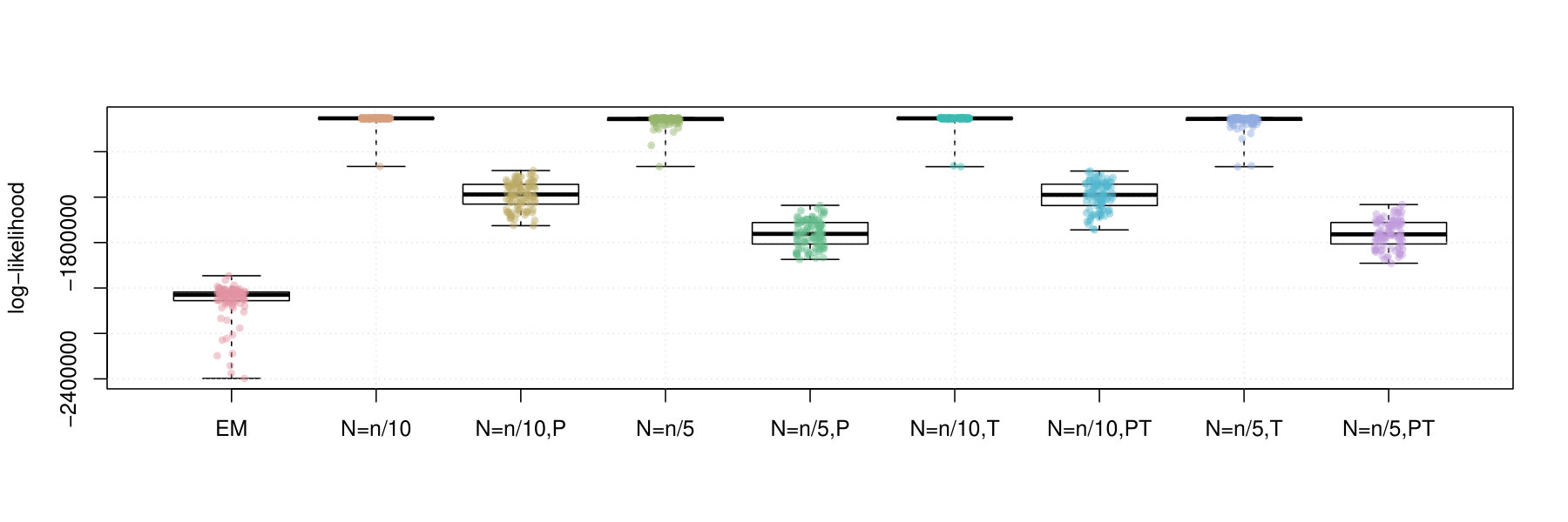 Figure 1
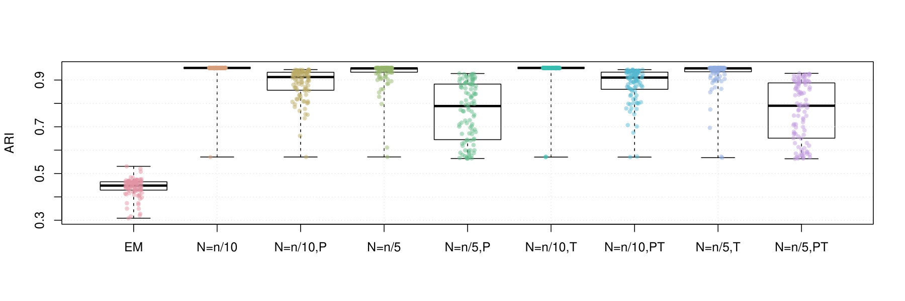 Figure 2
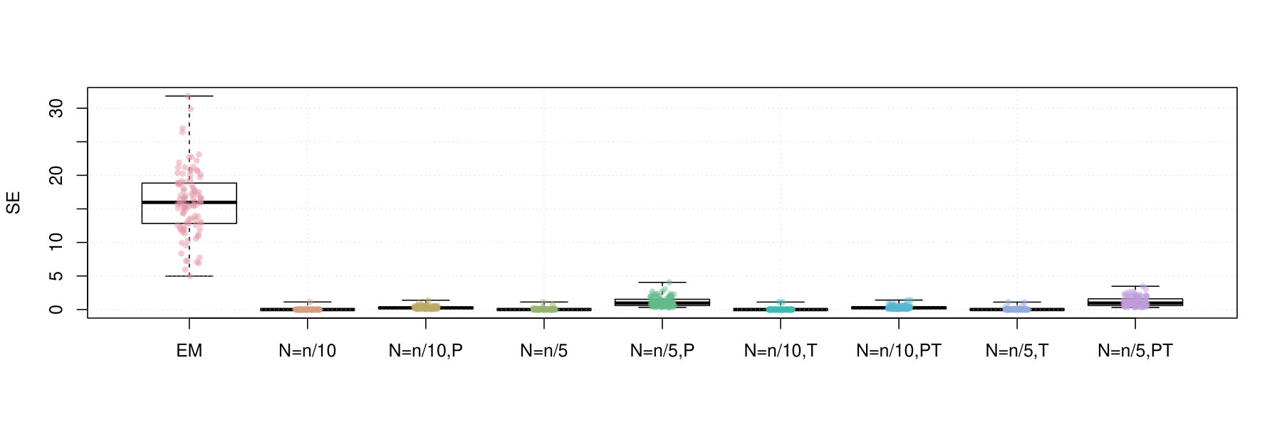 Figure 3
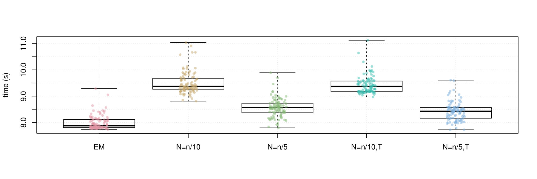 Figure 4
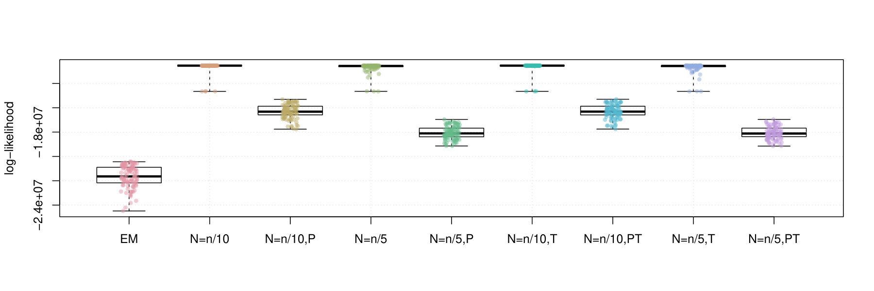 Figure 5
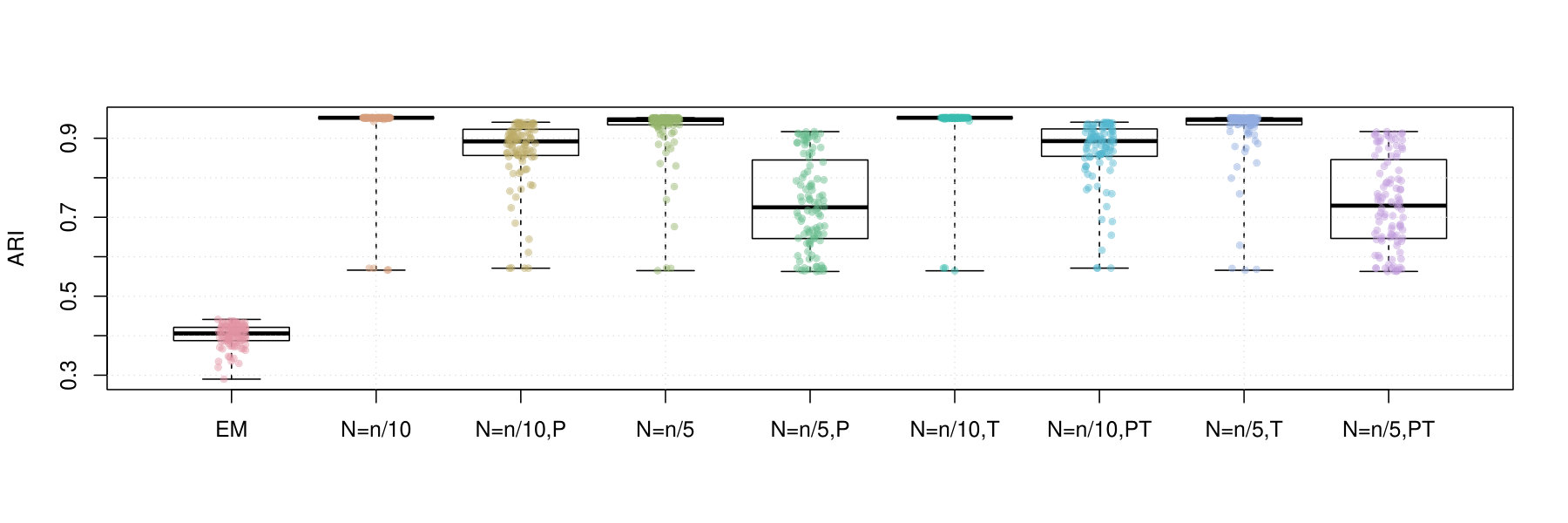 Figure 6
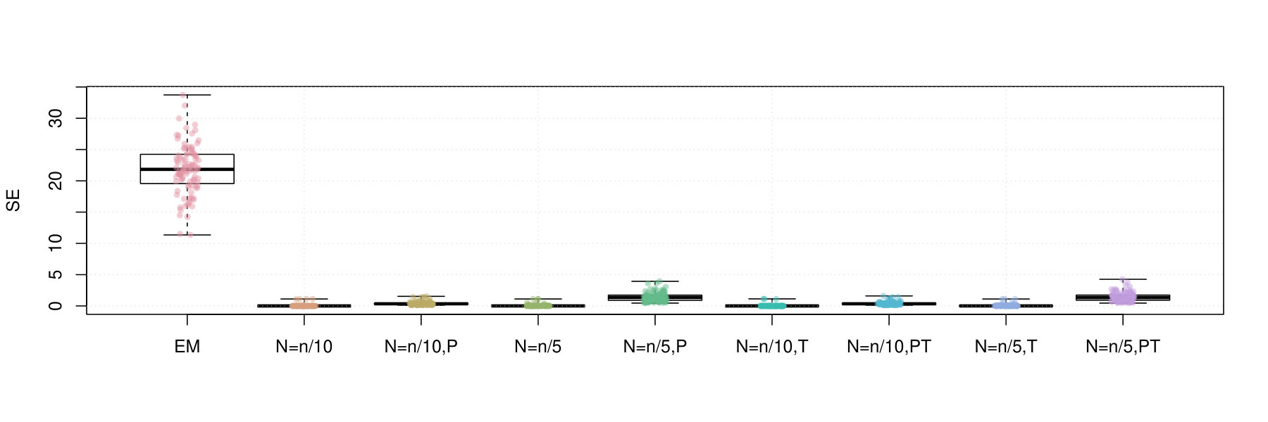 Figure 7
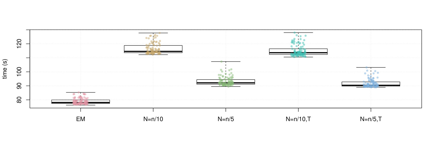 Figure 8
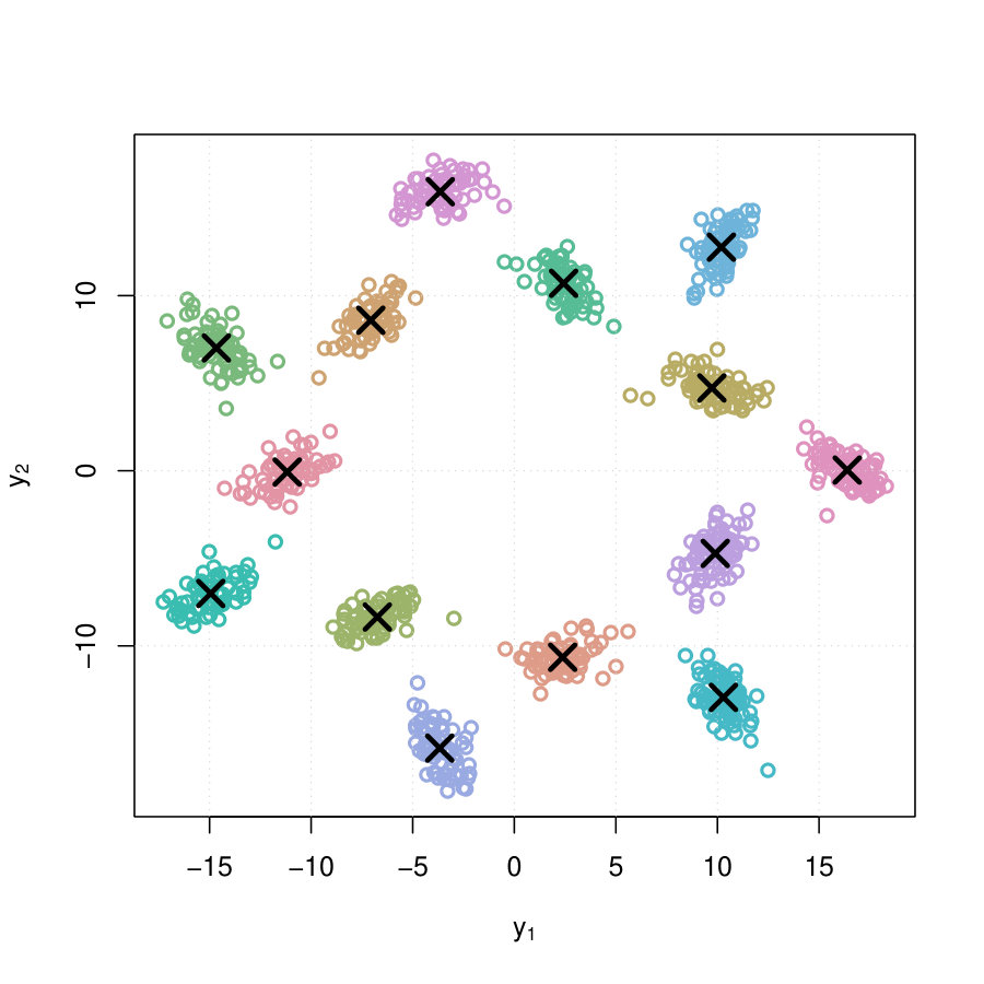 Figure 9
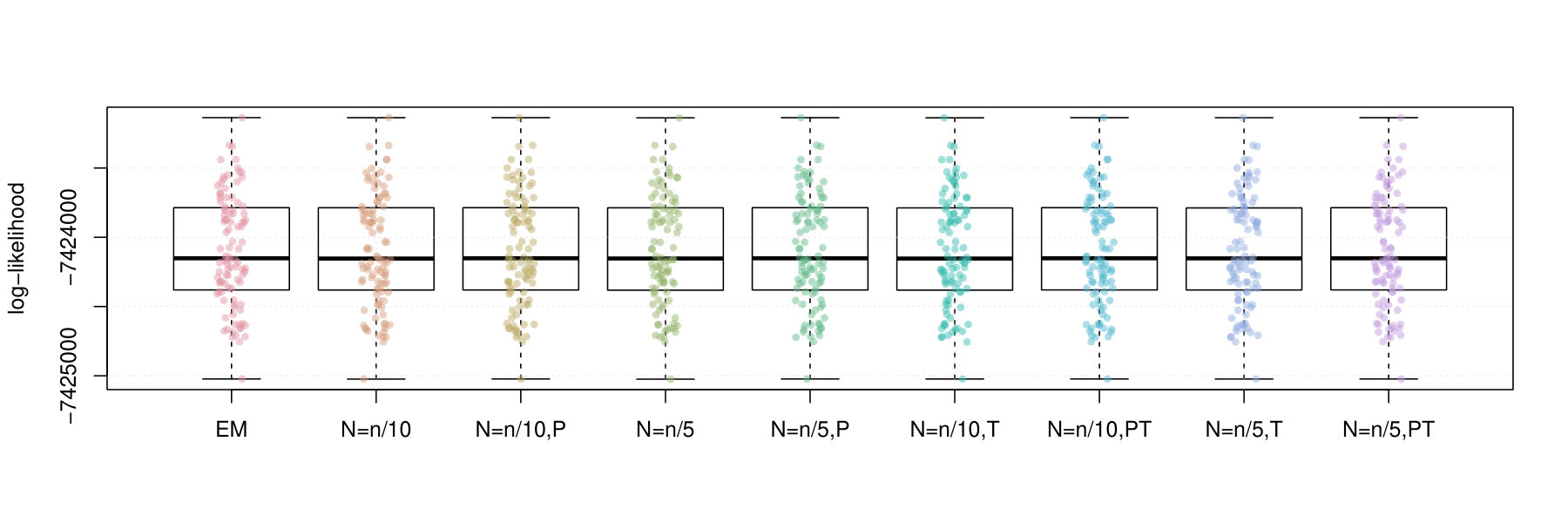 Figure 10
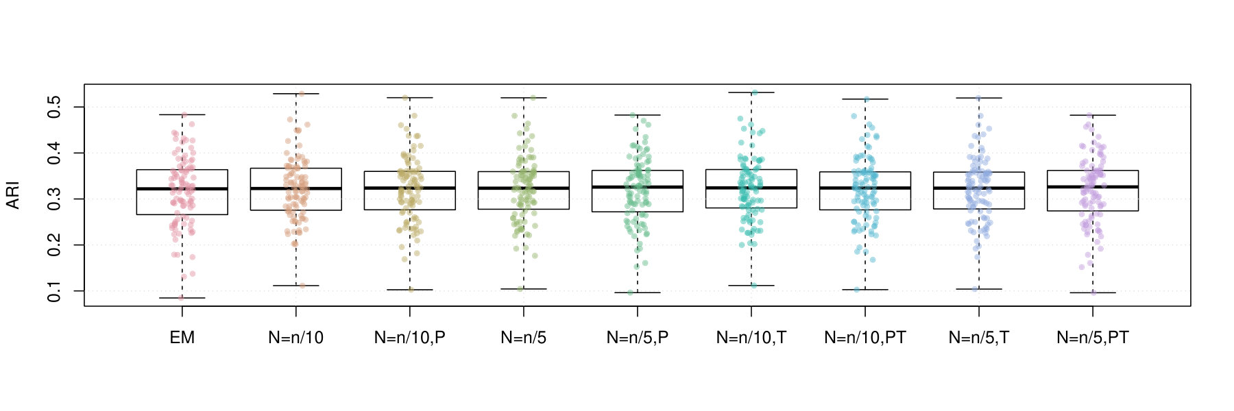 Figure 11
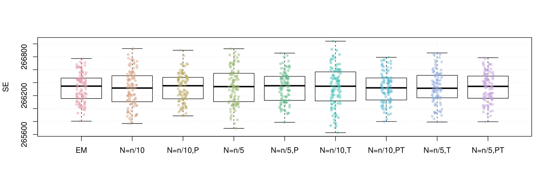 Figure 12
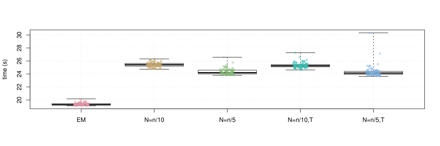 Figure 13
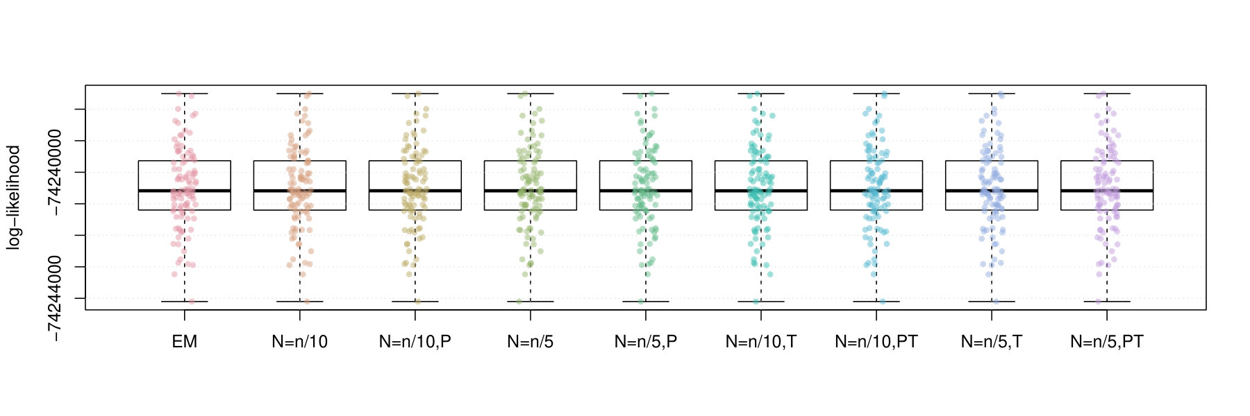 Figure 14
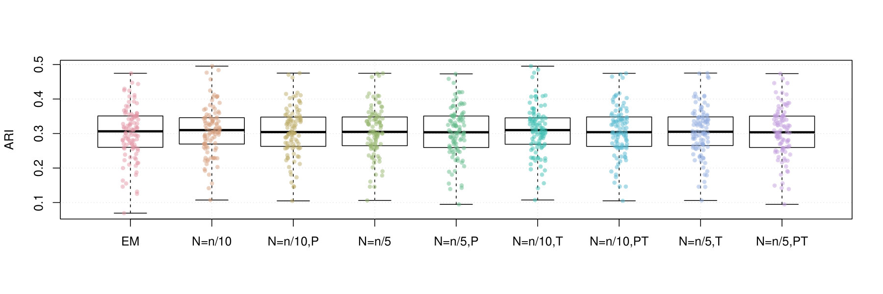 Figure 15
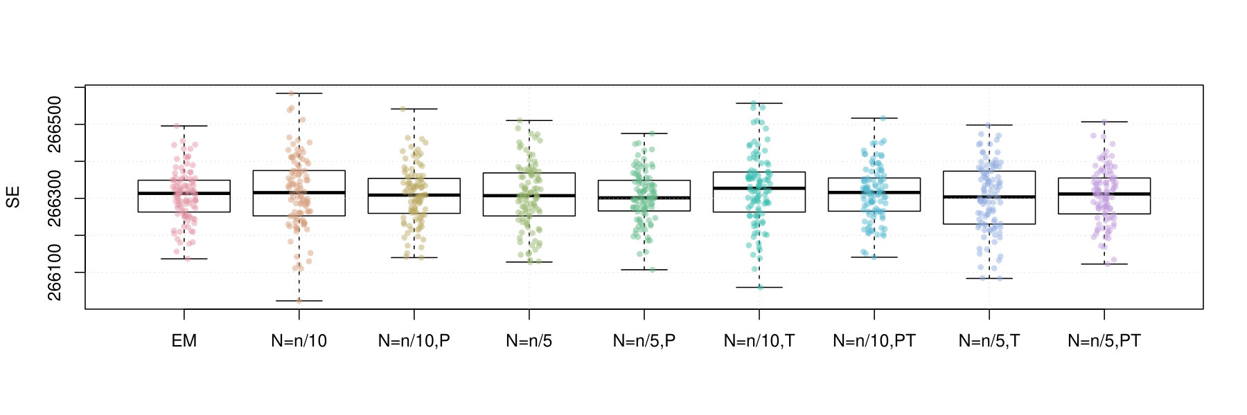 Figure 16
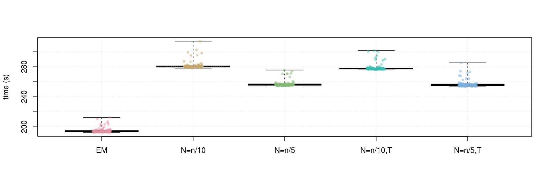 Figure 17
| ARI | log-likelihood | |||||||
|---|---|---|---|---|---|---|---|---|
| EM | Mini | Mini Pol | EM | Mini | Mini Pol | |||
| 10 | Mean | 0.401 | 0.443 | 0.432 | 0.352 | -4.98E+06 | -4.96E+06 | -5.01E+06 |
| SE | 0.004 | 0.004 | 0.004 | 0.002 | 1.19E+03 | 6.43E+02 | 5.90E+02 | |
| 20 | Mean | 0.436 | 0.475 | 0.480 | 0.367 | -9.46E+06 | -9.44E+06 | -9.52E+06 |
| SE | 0.005 | 0.005 | 0.005 | 0.002 | 2.20E+03 | 1.37E+03 | 1.67E+03 | |
| 50 | Mean | 0.394 | 0.434 | 0.438 | 0.369 | -2.18E+07 | -2.17E+07 | -2.20E+07 |
| SE | 0.005 | 0.005 | 0.006 | 0.002 | 8.47E+03 | 7.01E+03 | 4.85E+03 | |
| 100 | Mean | 0.326 | 0.356 | 0.377 | 0.372 | -3.99E+07 | -3.97E+07 | -4.05E+07 |
| SE | 0.004 | 0.004 | 0.005 | 0.002 | 1.83E+04 | 1.68E+04 | 8.72E+03 |
Peer Reviews
No public reviews on file for this paper yet. If you reviewed it on a platform where reviews are public (OpenReview, ICLR, NeurIPS, ICML), you can paste yours below so the community can read it here.
Videos
No videos yet. Explain this paper in a talk, walkthrough, or lecture? Add one.
Taxonomy
TopicsBayesian Methods and Mixture Models · Machine Learning and Algorithms · Statistical Methods and Inference
Mini-batch learning of exponential family finite mixture models
Hien D. Nguyen1∗, Florence Forbes2, and Geoffrey J. McLachlan3
Abstract
Mini-batch algorithms have become increasingly popular due to the requirement for solving optimization problems, based on large-scale data sets. Using an existing online expectation–maximization (EM) algorithm framework, we demonstrate how mini-batch (MB) algorithms may be constructed, and propose a scheme for the stochastic stabilization of the constructed mini-batch algorithms. Theoretical results regarding the convergence of the mini-batch EM algorithms are presented. We then demonstrate how the mini-batch framework may be applied to conduct maximum likelihood (ML) estimation of mixtures of exponential family distributions, with emphasis on ML estimation for mixtures of normal distributions. Via a simulation study, we demonstrate that the mini-batch algorithm for mixtures of normal distributions can outperform the standard EM algorithm. Further evidence of the performance of the mini-batch framework is provided via an application to the famous MNIST data set.
1Department of Mathematics and Statistics, La Trobe University, Melbourne, Victoria, Australia.
2Univ. Grenoble Alpes, Inria, CNRS, Grenoble INP*†*, LJK, 38000 Grenoble, France. *†*Institute of Engineering Univ. Grenoble Alpes.
3School of Mathematics and Physics, University of Queensland, St. Lucia, Brisbane, Australia.
*∗*Corresponding author: Hien Nguyen (Email: [email protected]).
**Key words: **expectation–maximization algorithm, exponential family distributions, finite mixture models, mini-batch algorithm, normal mixture models, online algorithm
1 Introduction
The exponential family of distributions is an important class of probabilistic models with numerous applications in statistics and machine learning. The exponential family contains many of the most commonly used univariate distributions, including the Bernoulli, binomial, gamma, geometric, inverse Gaussian, logarithmic normal, Poisson, and Rayleigh distributions, as well as multivariate distributions such as the Dirichlet, multinomial, multivariate normal, von Mises, and Wishart distributions. See Forbes et al., (2011, Ch. 18), DasGupta, (2011, Ch. 18), and Amari, (2016, Ch. 2).
Let be a random variable (with realization ) on the support () , arising from a data generating process (DGP) with probability density/mass function (PDF/PMF) that is characterized by some parameter vector (). We say that the distribution that characterizes the DGP of is in the exponential family class, if the PDF/PMF can be written in the form
[TABLE]
where and are -dimensional vector functions, and and are functions of and , respectively. If the dimensionality of and is less than , then we say that the distribution that characterizes the DGP of is in the curved exponential class.
Let (; ) be a latent random variable, and write . Suppose that the PDF/PMF of can be written as , for each . If we assume that , such that , then we can write the marginal PDF/PMF of in the form
[TABLE]
where we put the unique elements of and into . We call the -component finite mixture PDF, and we call the component PDF, characterized by the parameter vector , where is some subset of a real product space. We also say that the elements are prior probabilities, corresponding to the respective component.
The most common finite mixtures models are mixtures of normal distributions, which were popularization by Pearson, (1894), and have been prolifically used by numerous prior authors (cf. McLachlan et al.,, 2019). The -component -dimensional normal mixture model has PDF of the form
[TABLE]
where the normal PDFs
[TABLE]
replace the component densities , in (2). Each component PDF (4) is parameterized by a mean vector and a positive-definite symmetric covariance matrix . We then put each , , and into the vector .
As earlier noted, the normal distribution is a member of the exponential family, and thus (4) can be written in form (1). This can be observed by putting the unique elements of and into , and writing in form (1), with mappings
[TABLE]
[TABLE]
When conducting data analysis using a normal mixture model, one generally observes an independent and identically (IID) sequence of observations , arising from a DGP that is hypothesized to be characterized by a PDF of the form (3), with unknown parameter vector . The inferential task is to estimate via some estimator that is computed from . The most common computational approach to obtaining an estimator of is via maximum likelihood (ML) estimation, using the expectation–maximization algorithm (EM; Dempster et al.,, 1977). See McLachlan & Peel, (2000, Ch. 3.2) for a description of the normal mixture EM algorithm. Generally, when , , and are of small to moderate size, the conventional EM approach is feasible, and is able to perform the task of ML estimation in a timely manner. Unfortunately, due to its high memory demands, costly matrix operations (Nguyen & McLachlan,, 2015), and slow convergence rates (McLachlan & Krishnan,, 2008, Sec. 3.9), the conventional EM algorithm is not suited for the computational demands of analyzing increasingly large data sets, such as those that could be considered as big data in volumes such as Buhlmann et al., (2016), Han et al., (2017), and Hardle et al., (2018).
Over the years, numerous algorithms have been proposed as means to alleviate the computational demands of the EM algorithm for normal mixture models. Some of such approaches include the component-wise algorithm of Celeux et al., (2001), the greedy algorithm of Vlassis & Likas, (2002), the sparse and incremental -tree algorithm of Ng & McLachlan, (2004), the subspace projection algorithm of Bouveyron et al., (2007), and the matrix operations-free algorithm of Nguyen & McLachlan, (2015).
There has been a recent resurgence in stochastic approximation algorithms, of the Robbins & Monro, (1951) and Kiefer & Wolfowitz, (1952) type, developed for the purpose of solving computationally challenging optimization problems, such as the ML estimation of normal mixture models. A good review of the current literature can be found in Chau & Fu, (2015). Naïve and direct applications of the stochastic approximation approach to mixture model estimation can be found in Liang & Zhang, (2008), Zhang & Liang, (2008), and Nguyen & Jones, (2018).
Following a remark from Cappé & Moulines, (2009) regarding the possible extensions of the online EM algorithm, we propose mini-batch EM algorithms for the ML estimation of exponential family mixture models. These algorithms include a number of variants, among which are update truncation variants that had not been made explicit, before. Using the theorems from Cappé & Moulines, (2009), we state results regarding the convergence of our algorithms. We then specialize our attention to the important case of normal mixture models, and demonstrate that the required assumptions for convergence are met in such a scenario.
A thorough numerical study is conducted in order to assess the performance of our normal mixture mini-batch algorithms. Comparisons are drawn between our algorithms and the usual batch EM algorithm for ML estimation of normal mixture models. We show that our mini-batch algorithms can be applied to very large data sets by demonstrating its applicability to the ML estimation of normal mixture models on the famous MNIST data of LeCun et al., (1998).
References regarding mixtures of exponential family distributions and EM-type stochastic approximation algorithms, and comments regarding some recent related literature are relegated to the Supplementary Materials, in the interest of brevity. Additional remarks, numerical results, and derivations are also included in these Supplementary Materials in order to provide extra context and further demonstrate the capabilities of the described framework. These demonstrations include the derivation of mini-batch EM algorithms for mixtures of exponential and Poisson distributions. The Supplementary Materials can be found at https://github.com/hiendn/StoEMMIX/blob/master/Manuscript_files/SupplementaryMaterials.pdf.
The remainder of the paper is organized as follows. In Section 2, we present the general results of Cappé & Moulines, (2009) and demonstrate how they can be used for mini-batch ML estimation of exponential family mixture models. In Section 3, we derive the mini-batch EM algorithms for the ML estimation of normal mixtures, as well as verify the convergence of the algorithms using the results of Cappé & Moulines, (2009). Via numerical simulations, we compare the performance of our mini-batch algorithms to the usual EM algorithm for ML estimation of normal mixture models, in Section 4. A set of real data study on a very large data set is presented in Section 5. Conclusions are drawn in Section 6. Additional material, such as mini-batch EM algorithms for exponential and Poisson mixture models, can be found in the Supplementary Materials.
2 The mini-batch EM algorithm
Suppose that we observe a single pair of random variables , where is observed but is latent, where and are subsets of multivariate real-valued spaces. Furthermore, suppose that the marginal PDF/PMF of is hypothesized to be of the form , for some unknown parameter vector . A good estimator for is the ML estimator that can be defined as:
[TABLE]
When the problem (7) cannot be solved in a simple manner (e.g. when the solution does not exist in closed form), one may seek to employ an iterative scheme in order to obtain an ML estimator. If the joint PDF/PMF of is known, then one can often construct an EM algorithm in order to solve the problem in the bracket of (7).
Start with some initial guess for and call it the zeroth iterate of the EM algorithm and suppose that we can write the point PDF/PMF of as , for any . At the iterate of the EM algorithm, we perform an expectation (E-) step, followed by a maximization (M-) step. The E-step consists of obtaining the conditional expectation of the complete-data log-likelihood (i.e. ) given the observed data, using the current estimate of the parameter vector
[TABLE]
which we will call the conditional expected complete-data log-likelihood.
Upon obtaining the conditional expectation of the complete-data log-likelihood, one then conducts the M-step by solving the problem
[TABLE]
The E- and M-steps are repeated until some stopping criterion is met. Upon termination, the final iterate of the algorithm is taken as a solution for problem (7). See McLachlan & Krishnan, (2008) for a thorough exposition regarding the EM algorithm.
2.1 The online EM algorithm
Suppose that we observe a sequence of IID replicates of the variable , , where each is the visible component of the pair (). In the online learning context, each of the observations from is observed one at a time, in sequential order.
Using the sequentially obtained sequence , we wish to obtain an ML estimator for the parameter vector , in the same sense as in (7). In order to construct an online EM algorithm framework with provable convergence, Cappé & Moulines, (2009) assume the following restrictions regarding the nature of the hypothesized DGP of .
- A1
The complete-data likelihood corresponding to the pair is of exponential family form. That is,
[TABLE]
where , , , and are as defined for (1).
- A2
The function
[TABLE]
is well defined for all and .
- A3
There exists a convex open subset , which satisfies the properties that:
- (i)
for all , , , for any , and
- (ii)
for any , the function
[TABLE]
has a unique global maximum over , which will be denoted by
[TABLE]
Let be the expected complete-data log-likelihood over data , at the E-step of an EM algorithm for solving the problem:
[TABLE]
where we say that is the ML estimator, based on the data . When, A1–A3 are satisfied, we can write
[TABLE]
which can then be maximized, with respect to , in order to yield an M-step update of the form:
[TABLE]
where is a function that depends only on the average .
Now we suppose that we sample the individual observations of , one at a time and sequentially. Furthermore, upon observation of , we wish to compute an online estimate of , which we denote as . Based on the simplification of the EM algorithm under A1–A3, as described above, Cappé & Moulines, (2009) proposed the following online EM algorithm.
Upon observation of , compute the intermediate updated sufficient statistic
[TABLE]
with . Here, is the term of the learning rate sequence that we will discuss in further details in the sequel. Observe that we can also write
[TABLE]
which makes it clear that for , is a weighted average between and . Using and the function , we can then express the iteration online EM estimate of as
[TABLE]
Next, we state a consistency theorem that strongly motivates the use of the online EM algorithm, defined by (11) and (12). Suppose that the true DGP that generates each of is characterized by the probability measure . Write the expectation operator with respect to this measure as . In order to state the consistency result of Cappé & Moulines, (2009), we require the following additional set of assumptions.
- B1
The parameter space is a convex and open subset of a real product space, and the functions and , in (8), are both twice continuously differentiable with respect to .
- B2
The function , as defined in (10), is a continuously differentiable function with respect to , where is as defined in A3.
- B3
For some , and all compact ,
[TABLE]
As the algorithm defined by (11) and (12) is of the Robbins-Monro type, establishment of convergence of the algorithm requires the definition of a mean field (see Chen,, 2003 and Kushner & Yin,, 2003 for comprehensive treatments regarding such algorithms). In the case of the online EM algorithm, we write the mean field as
[TABLE]
and define the set of its roots as .
Define the log-likelihood of the hypothesized PDF with respect to the measure , as
[TABLE]
Let denote the gradient with respect to , and define the sets
[TABLE]
and
[TABLE]
Note that is the set of stationary points of the log-likelihood function. Further, define the distance between a real vector and a set by
[TABLE]
where is the usual Euclidean metric, and denote the complement of a subset of a real product space by . Finally, make the following assumptions.
- C1
The sequence of learning rates fulfills the conditions that , for each ,
[TABLE]
- C2
At initialization and, with probability 1,
[TABLE]
- C3
The set is nowhere dense.
Theorem 1** (Cappe and Moulines, 2009).**
Assume that A1–A3, B1–B3, and C1–C3 are satisfied, and let be an IID sample with DGP characterized by the PDF , which is hypothesized to have the form , as in (8). Further, let and be sequences generated by the online EM algorithm, defined by (11) and (12). Then, with probability 1,
[TABLE]
Notice that this result allows for a mismatch between the true probability measure and the assumed pseudo-true family from which is hypothesized to arise. This therefore allows for misspecification, in the sense of White, (1982), which is almost certain to occur in the modeling of any sufficiently complex data. In any case, the online EM algorithm will converge towards an estimate of the parameter vector , which is in the set . When the DGP can be characterized by a density in the family of the form , we observe that contains not only the global maximizer of the log-likelihood function, but also local maximizers, minimizers, and saddle points. Thus, the online algorithm suffers from the same lack of strong convergence guarantees, as the batch EM algorithm (cf. Wu,, 1983).
In the case of misspecification the set will include the parameter vector that maximizes the log-likelihood function, with respect to the true probability measure . However, as with the well-specified case, it will also include stationary points of other types, as well. We further provide characterizations of the sets and in terms of the Kullback-Leibler divergence (KL; Kullback & Leibler,, 1951) in the Supplementary Materials.
Assumption C1 can be fulfilled by taking sequences of form , for some and . We shall discuss this point further, in the sequel. Although the majority of the assumptions can be verified or are fulfilled by construction, the two limits in C2 stand out as being particularly difficult to verify. In Cappé & Moulines, (2009), the authors suggest that one method for enforcing C2 is to use the method of update truncation, but they did not provide an explicit scheme for conducting such truncation.
A truncation version of the algorithm defined by (11) and (12) can be specified via the method of Delyon et al., (1999). That is, let be a sequence of compact sets, such that
[TABLE]
We then replace (11) and (12) by the following scheme. At the iteration, firstly compute
[TABLE]
Secondly,
[TABLE]
else
[TABLE]
where is an arbitrary random sequence, such that , for each . We have the following result regarding the algorithm defined by (15)–(17).
Proposition 1**.**
Assume that A1–A3, B1–B3, C1 and C3 are satisfied, and let be an IID sample with DGP characterized by the PDF , which is hypothesized to have the form , as in (8). Further, let and be sequences generated by the truncated online EM algorithm, defined by (15)–(17). Then, with probability 1,
[TABLE]
The proof of Proposition 1 requires the establishment of equivalence between A1–A3, B1–B3, C1, and C3, and the many assumptions of Theorem 3 and 6 of Delyon et al., (1999). Thus the proof is simple and mechanical, but long and tedious. We omit it for the sake of brevity.
2.2 The mini-batch algorithm
At the most elementary level, a mini-batch algorithm for computation of a sequence of estimators for some parameter , from some sample , where , has the following property. The algorithm is iterative, and at the iteration of the algorithm, the estimator only depends on the previous iterate and some subsample, possibly with replacement, of . Typical examples of mini-batch algorithms include the many variants of the stochastic gradient descent-class of algorithms; see, for example, Cotter et al., (2011), Li et al., (2014), Zhao et al., (2014), and Ghadimi et al., (2016).
Suppose that we observe a fixed size realization of some IID random sample . Furthermore, fix a so-called batch size and a learning rate sequence , and select some appropriate initial values and from which the sequences and can be constructed. A mini-batch version of the online EM algorithm, specified by (11) and (12) can be specified as follows. For each , sample observations from uniformly, with replacement, and denote the subsample by . Then, using , compute
[TABLE]
In order to justify the mini-batch algorithm, we make the following observation. The online EM algorithm, defined by (11) and (12), is designed to obtain a root in the set , which is a vector such that
[TABLE]
If (i.e., the case proposed in Cappé & Moulines,, 2009, Sec. 2.5), then the DGP for generating subsamples is simply a single draw from the empirical measure:
[TABLE]
where is the Dirac delta function (see, for details, Prosperetti,, 2011, Ch. 2). We can write
[TABLE]
which is the log-likelihood function, with respect to the realization , under the density function of form . Thus, in the case, the algorithm defined by (18) solves for log-likelihood roots of the form
[TABLE]
or equivalently, solving for an element in the set
[TABLE]
The case follows the same argument, and is described in the Supplementary Materials (Section 2.2). Let denote the probability measure corresponding to the DGP of independent random samples from . We have the following result, based on Theorem 1.
Corollary 1**.**
For any , assume that A1–A3, B1–B3, and C1–C3 are satisfied (replacing by , and by , where appropriate), and let be a realization of some IID random sequence , where each is hypothesized to arise from a DGP having PDF of the form , as in (8). Let and be sequences generated by the mini-batch EM algorithm, defined by (11) and (12). Then, with probability 1,
[TABLE]
That is, as we take , the algorithm defined by (11) and (12) will identify elements in the sets and , with probability 1. As with the case of Theorem 1, C2 is again difficult to verify. Let be as per (14). Then, we replace the algorithm defined via (18), by the following truncated version.
Again, suppose that we observe a fixed size realization of some IID random sample . Furthermore, fix a so-called batch size and a learning rate sequence , and select some appropriate initial values and from which the sequences and can be constructed. For each , sample observations from uniformly, with replacement, and denote the subsample by . Using , compute
[TABLE]
Then, with being appropriately replaced by , use (16) and (17) to compute and . We obtain the following result via an application of Proposition 1.
Corollary 2**.**
For any , assume that A1–A3, B1–B3, and C1–C3 are satisfied (replacing by , and by , where appropriate), and let be a realization of some IID random sequence , where each is hypothesized to arise from a DGP having PDF of the form , as in (8). Let and be sequences generated by the truncated mini-batch EM algorithm, defined by (20), (16), and (17). Then, with probability 1,
[TABLE]
2.3 The learning rate sequence
As previously stated, a good choice for the learning rate sequence is to take , for each , such that and . Under the assumptions of Theorem 1, Cappé & Moulines, (2009, Thm. 2) showed that the learning rate choice leads to the convergence of the sequence , in distribution, to a normal distribution with mean and covariance matrix depending on , for some . Here is a sequence of online EM algorithm iterates, generated by (11) and (12). A similar result can be stated for the truncated online EM, mini-batch EM, and truncated mini-batch EM algorithms, by replacing the relevant indices and quantities in the previous statements by their respective counterparts.
The result above implies that the convergence rate is , for any valid , where is the usual order in probability notation (see White,, 2001, Defn. 2.33). Thus, it would be tempting to take in order to obtain a rate with optimal order of . However, as shown in Cappé & Moulines, (2009, Thm. 2), the case requires constraints on in order to fulfill a stability assumption that is impossible to validate, in practice.
It is, however, still possible to obtain a sequence of estimators that converges to some at a rate with optimal order . We can do this via the famous so-called Polyak averaging scheme of Polyak, (1990) and Polyak & Juditsky, (1992). In the current context, one takes as an input the sequence of online EM iterates , and output the running average sequence , where
[TABLE]
for each . For any , it is provable that . As before, this result generalizes to the cases of the truncated online EM, mini-batch EM, and truncated mini-batch EM algorithms, also.
We note that the computation of the running average term (21) does not require the storage of the entire sequence of iterates , as one would anticipate by applying (21) naïvely. One can instead write (21) in the iterative form
[TABLE]
3 Normal mixture models
3.1 Finite mixtures of exponential family distributions
We recall from Section 1, that the random variable is said to arise from a DGP characterized by a component finite mixture of component PDFs of form , if it has a PDF of the form (2). Furthermore, if the component PDFs are of the exponential family form (1), then we further write the PDF of as
[TABLE]
From the construction of the finite mixture model, we have the fact that (22) is the marginalization of the joint density of the random variable :
[TABLE]
over the random variable , recalling that is a categorical random variable with categories (cf. McLachlan & Peel,, 2000, Ch. 2). Here, \left\llbracket c\right\rrbracket is the Iverson bracket notation, that takes value 1 if condition is true, and 0 otherwise (Iverson,, 1967, Ch. 1). We rewrite (23) as follows:
[TABLE]
where , ,
[TABLE]
and thus obtain the following general result regarding finite mixtures of exponential family distributions.
Proposition 2**.**
The complete-data likelihood of any finite mixture of exponential family distributions with PDF of the form (22) can also be written in the exponential family form (8).
With Proposition 2, we have proved that when applying the online EM or the mini-batch EM algorithm to the problem of conducting ML estimation for any finite mixture model of exponential family distributions, A1 is automatically satisfied.
3.2 Finite mixtures of normal distributions
Recall from Section 1 that the random variable is said to be distributed according to a finite mixture of normal distributions, if it characterized by a PDF of the form (3). Using the exponential family decomposition from (5) and (6), we write the complete-data likelihood of in the form (8) by setting , ,
[TABLE]
where is the matrix vectorization operator.
Using the results from McLachlan & Peel, (2000, Ch. 3), we write the conditional expectation (9) in the form
[TABLE]
where
[TABLE]
is the usual a posteriori probability that (), given observation of . Again, via the results from McLachlan & Peel, (2000, Ch. 3), we write the update function in the following form. Define to have the elements and , for each , where each subsequently has elements and . Furthermore, for convenience, we define for the following notation
[TABLE]
and
[TABLE]
with
[TABLE]
Then the application of the M-step is equivalent to apply function as a function of , countaining the unique elements of , , and , for , defined by
[TABLE]
This implies that the mini-batch EM and truncated mini-batch EM algorithms proceed via update rule , where and are as given in (18). We start from and . Then, which has elements
[TABLE]
and
[TABLE]
3.3 Convergence analysis of the mini-batch algorithm
In addition to Assumptions A1–A3, B1–B3, and C1–C3, make the additional assumption
- D1
The Hessian matrix of , evaluated at any , is non-singular with respect to .
Assumption D1 is generally satisfied for all but pathological samples . The following result is proved in the Supplementary Materials.
Proposition 3**.**
Let be a realization of some IID random sequence , where each is hypothesized to arise from a DGP having PDF of the form (3). If and are sequences generated by the mini-batch EM algorithm, defined by (18) and (25), then for any , if C1, C2, and D1 are satisfied (replacing by , and by , where appropriate), then, with probability 1,
[TABLE]
Alternatively, if and are sequences generated by the truncated mini-batch EM algorithm, defined by (20), (16), (17) and (25), then for any , if C1 and D1 are satisfied (replacing by , and by , where appropriate), then, with probability 1,
[TABLE]
3.4 A truncation sequence
In order to apply the truncated version of the mini-batch EM algorithm, we require an appropriate sequence that satisfies condition (14). This can be constructed in parts. Let us write
[TABLE]
where we shall let ,
[TABLE]
[TABLE]
and
[TABLE]
using the notation and to denote the smallest and largest eigenvalues of the matrix . A justification regarding this truncation scheme can be found in the Supplementary Materials.
We make a final note that the construction (28) is not a unique method for satisfying the conditions of (14). One can instead, for example, replace , by () in the definitions of the sets that constitute (28).
4 Simulation studies
We present a pair of simulation studies, based upon the famous Iris data set of Fisher, (1936) and the Wreath data of Fraley et al., (2005), in the main text. A further four simulation scenarios are presented in the Supplementary Materials. In each case, we utilize the initial small data sets, obtained from the base R package (R Core Team,, 2018) and the mclust package for R (Scrucca et al.,, 2016), respectively, and use them as templates to generate much larger data sets. All computations are conducted in the R programming environment, although much of the bespoke programs are programmed in C and integrated in R via the Rcpp and RcppArmadillo packages of (Eddelbuettel,, 2013). Furthermore, timings of programs were conducted on a MacBook Pro with a 2.2 GHz Intel Core i7 processor, 16 GB of 1600 MHz DDR3 RAM, and a 500 GB SSD hard drive. We note that all of the code used to conduct the simulations and computations for this manuscript can be accessed from https://github.com/hiendn/StoEMMIX.
In the sequel, in all instances, we shall use the learning rate sequence , where , which follows from the choice made by Cappé & Moulines, (2009) in their experiments. In all computations, a fixed number of epochs (or epoch equivalence) of is allotted to each algorithm. Here, recall that the number of epochs is equal to the number of sweeps through the data set that an algorithm is allowed. Thus, drawing observations from the data , with replacement, is equivalent to 10 epochs. Thus, each iteration of the standard EM algorithm counts as a single epoch, whereas, for a mini-batch algorithm with batch size , every iterations counts as an epoch.
Next, in both of our studies, we consider batch sizes of and , we further consider Polyak averaging as well as truncation. Thus, for each study, a total of eight variants of the mini-batch EM algorithm is considered. In the truncate case, we set . Finally, the variants of the mini-batch EM algorithm are compared to the standard (batch) EM algorithm for fitting finite mixtures of normal distributions. In the interest of fairness, each of the algorithms is initialized at the same starting value of , using the randomized initialization scheme suggested in McLachlan & Peel, (2000, Sec. 3.9.3). That is, the same randomized starting instance is used for the EM algorithm and each of the mini-batch variants.
To the best of our knowledge, the most efficient and reliable implementation of the EM algorithm for finite mixtures of normal distributions, in R, is the em function from the mclust package. Thus, this will be used for all of our comparisons. Data generation from the template data sets is handled using the simdataset function from the MixSim package (Melnykov et al.,, 2012), in the Iris study, and the simVVV function from mclust in the Wreath study. Timing was conducted using the function.
4.1 Iris data
The Iris data (accessed in R via the data(iris) command) contain measurements of dimensions from 150 iris flowers, 50 of each are of the species Setosa, Versicolor, and Virginica, respectively. The 4 dimensions of each flower that are measured are petal length, petal width, sepal length, and sepal width. To each of the subpopulations of species, we fit a single multivariate normal distribution to the 50 observations (i.e., we estimate a mean vector and covariance matrix, for each species). Then, using the three mean vectors and covariance matrices, we construct a template component normal mixture model with equal mixing proportions (), of form (3). This template distribution is then used to generate synthetic data sets of any size .
Two experiments are performed using this simulation scheme. In the first experiment, we generate observations from the template. We then utilize and each of the truncated EM algorithm variants as well as the batch EM algorithm to compute ML estimates. We use a number of measures of performance for each algorithm variant. These include the computation time, the log-likelihood, the squared error of the parameter estimates (SE; the Euclidean distance as compared to the generative parameter vector), and the adjusted-Rand index (ARI; Hubert & Arabie,, 1985) between the maximum a posteriori clustering labels obtained from the fitted mixture model and the true generative data labels.
The ARI measures whether or not two sets of labels are in concordance or not. Here a value of 1 indicates perfect similarity, and 0 indicates discordance. Since the ARI allows for randomness in the labelling process, it is possible to have negative ARI values, which are rare and also indicates discordance in the data. Each variant is repeated times, and each performance measurement is recorded in order to obtain a measure of the overall performance of each algorithm. For future reference, we name this study Iris1. In the second study, which we name Iris2, we repeat the setup of Iris1 but with the number of observations increased to .
4.2 Wreath data
The Wreath data (accessed in R via the data(wreath) command) contain 1000 observations of dimensional vectors, each belonging to one of distinct but unlabelled subpopulations. We use the Mclust function from mclust to fit a 14 component mixture normal distributions to the data. The data, along with the means of the subpopulation normal distributions, are plotted in Figure 1. Here, each observation is colored based upon the subpopulation that maximizes its a posteriori probability.
As with the Iris data, using the fitted mixture model as a template, we can then simulate synthetic data sets of any size . We perform two experiments using this scheme. In the first experiment, we simulate observations and assess the different algorithms, based on the computation time, the log-likelihood, the SE, and the ARI over Rep=100 repetitions, as per Iris1. We refer to this experiment as Wreath1. In the second experiment, we repeat the setup of Wreath1, but with , instead. We refer to this case as Wreath2.
4.3 Results
Figures 2 and 3 contain box plots that summarize the results of Iris1 and Iris2, respectively. Similarly, Figures 4 and 5 contain box plots that summarize the results of Wreath1 and Wreath2, respectively.
Firstly, we note that Polyak averaging requires no additional computational effort, for a given value of . Thus, we do not require separate timing data for Polyak averaging variants of the mini-batch EM algorithms in each of Figures 2–5. From the timing results, we observe that the standard EM algorithm is faster than the mini-batch versions, in all scenarios, regardless of the fact that all of the algorithms were computed using 10 epochs worth of data access. This is because the mini-batch algorithms require more additional intermediate steps in each algorithm loop (e.g., random sampling from the empirical distribution), as well as a multiplicative factor of more loops. From the plots, we observe that the larger value of tends to result in smaller computing times. There appears to be no difference in timing between the use of truncation or not.
In the Iris1 and Iris2 studies, we observe that the mini-batch EM algorithms uniformly outperform the standard EM algorithm in terms of the log-likelihood, SE, and ARI. In all three measurements, we observe that performed better than , and also that there were no differences between truncated versions of the mini-batch algorithms and equivalent variants without truncation. Polyak averaging appears to reduce the performance of the mini-batch algorithms, for a given level of , with respect to each of the three measurements.
In the Wreath1 and Wreath2 studies, we observe that the standard and mini-batch EM algorithms perform virtually the same across the log-likelihood, SE, and ARI metrics. This is likely due to the high degree of separability of each of the mixture components of the Wreath data, in comparison to the overlapping components of the Iris data. Our observation is true for all of the mini-batch EM variants, with or without truncation or Polyak averaging. Upon first impression, this may appear as a weakness of the mini-batch EM algorithm, since it produces the same performance while requiring more computational time. However, we must also remember that the mini-batch EM algorithm does not require all of the data to be stored in memory at each iteration of algorithm, whereas the EM algorithm does. Thus, the mini-batch algorithm is feasible in very large data situations, since it only requires a fixed memory size, of order , regardless of sample size , whereas the standard EM algorithm has a memory requirement that increases with .
To expand upon our currently presented results, we have also included a further two simulation studies regarding the fitting of finite mixtures of normal distributions using mini-batch EM algorithms. Our two studies are based on the Flea data of Wickham et al., (2011), a test scenario from the ELKI project of Schubert et al., (2015), and an original data generating process. The ELKI scenario is chosen due to its separability, in order to assess whether our conclusion regarding Wreath1 and Wreath2 are correct. The Flea data shares similarities with the Iris data but is higher dimensional. In all cases, we found that the mini-batch algorithms tended to outperform the EM algorithm in all but timing, on average. Detailed assessments of these studies can be found in the Supplementary Materials.
In addition, we have also investigated the use of the mini-batch EM algorithm for estimation of non-normal mixture models. Namely, we present a pair of algorithms for the estimation of exponential and Poisson mixture models. We demonstrate their performance via an additional pair of simulation studies.
To conclude, we make the following recommendations. Firstly, smaller batch sizes appear to yield higher likelihood values. Secondly, averaging appears to slow convergence of the algorithm to the higher likelihood value and is thus not recommended. Thirdly, truncation appears to have no effect on the performance. This is likely due to the fact that truncation may not have been needed in any of the experiments. In any case, it is always useful to use the truncated version of the algorithm, in case there are unforeseen instabilities in the optimization process. And finally, the standard EM algorithm may be preferred to the mini-batch EM algorithm when sample sizes are small and when the data are highly separable. However, even in the face of high separability, for large , it may not be feasible to conduct estimation by the standard EM algorithm and thus the mini-batch algorithms may be preferred due to feasibility.
It is interesting to observe that Polyak averaging tended to diminish the performance of the algorithms, in our studied scenarios. This is in contradiction to the theory that suggests that Polyak averaging should in fact increase the convergence rate to stationary solutions. We note, however, that the theory is asymptotic and the number of epochs that were used may be too short for the advantages of Polyak averaging to manifest, in practice.
5 Real data study
5.1 MNIST data
The MNIST data of LeCun et al., (1998) consists of observations of pixel images of handwritten digits. These handwritten digits were sampled nearly uniformly. That is there were 6903, 7877, 6990, 7141, 6824, 6313, 6876, 7293, 6825, and 6958 observations of the digits 0–9, respectively.
Next, it is notable that not all pixels are particularly informative. In fact, there is a great amount of redundancy in the dimensions. Out of the pixels, 65 are always zero, for every observation. Thus, the dimensions of the data are approximately 8.3% sparse.
We eliminate the spare pixels across all images to obtain a dense dimensionality of . Using the dimensions of the data, we conduct a principal component analysis (PCA) in order to further reduce the data dimensionality; see Jolliffe,, 2002 for a comprehensive treatment on PCA. Using the PCA, we extract the principal components (PCs) of each observation, and for various number of PCs . We can then use the data sets of observations and dimension , to estimate mixture of normal distributions for various values of .
5.2 Experimental setup
In the following study, we utilize only the truncated version of the mini-batch algorithm, having drawn the conclusions, from Section 4, that there appeared to be no penalty in performance due to truncation in practice. Again, drawing upon our experience from Section 4, we set as the batch size in all applications. The same learning rate sequence of , where is also used, and .
We apply the mini-batch algorithm to data with . Initialization of the parameter vector was conducted via the randomization scheme of McLachlan & Peel, (2000, Sec. 3.9.3). The mini-batch algorithm was run 100 times for each and the log-likelihood values were recorded for both the fitted models using the Polyak averaging and no averaging versions of the algorithm. The standard EM algorithm, as applied via the em function of the mclust package is again used for comparison. Each of the algorithms, including the algorithm, were initialized from the same initial randomization, in the interest of fairness, for each of the 100 runs. That is, a random partition of the data is generated once for each of the 100 runs, and the initial parameters for the EM, mini-batch and algorithms are all computed from the same initialization. The log-likelihood values of the standard and mini-batch EM algorithms are compared along with the ARI values. Algorithms are run for 10 epochs.
We compute the ARI values obtained when comparing the maximum *a posteriori *clustering labels, obtained from each of the algorithms (cf. McLachlan & Peel,, 2000, Sec. 1.15), and the true digit classes of each of the images. For a benchmark, we also compare the performance of the three EM algorithms with the algorithm, as applied via the kmeans function in R, which implements the algorithm of Hartigan & Wong, (1979). For fairness of comparison, we also allow the algorithm 10 epochs in each of 100 runs. As in Section 4, we note that all codes are available at https://github.com/hiendn/StoEMMIX, for the sake of reproducibility and transparency.
5.3 Results
The results from the MNIST experiment are presented in Table 1. We observe that for , all three EM variants provided better ARI than the algorithm. The best ARI values for all three EM algorithms occur when . When , the algorithm provided a better ARI, which appeared to be somewhat uniform across the four values of .
Among the EM algorithms, the mini-batch algorithm provided better ARI values, with the two variants not appearing to be significantly different from one another, when considering the standard errors of the ARI values, when . When , we observe that no averaging yielded a better ARI, whereas, when , averaging appeared to be better, on average.
Regarding the log-likelihoods, the mini-batch EM algorithm, when applied without averaging, uniformly and significantly outperformed the standard EM algorithm. On the contrary, when applied with averaging, the EM algorithm uniformly and significantly outperformed the mini-batch algorithm. This is also in contrary with what was observed in Section 4. This is an interesting result considering that the ARI of the mini-batch algorithm, with averaging, is still better than that of the EM algorithm. As in Section 4, we can recommend the use of the mini-batch EM algorithm without averaging, as it tends to outperform the standard EM algorithm for fit and is also yields better clustering outcomes, when measured via the ARI.
6 Conclusions
In Section 2, we reviewed the online EM algorithm framework of Cappé & Moulines, (2009), and stated the key theorems that guarantee the convergence of algorithms that are constructed under the online EM framework. We then presented a novel interpretation of the online EM algorithm that yielded our framework for constructing mini-batch EM algorithms. We then utilized the theorems of Cappé & Moulines, (2009) in order to produce convergence results for this new mini-batch EM algorithm framework. Extending upon some remarks of Cappé & Moulines, (2009), we also made rigorous the use of truncation in combination with both the online EM and mini-batch EM algorithm frameworks, using the construction and theory of Delyon et al., (1999).
In Section 3, we demonstrated how the mini-batch EM algorithm framework could be applied to construct algorithms for conducting ML estimation of finite mixtures of exponential family distributions. A specific analysis is made of the particularly interesting case of the normal mixture models. Here, we validate the conditions that permit the use of the Theorems from Section 2 in order to guarantee the convergence of the mini-batch EM algorithms for ML estimation of normal mixture models.
In Section 4, we conducted a set of four simulation studies in order to study the performance of the mini-batch EM algorithms, implemented in eight different variants, as compared to the standard EM algorithm for ML estimation of normal mixture models. There, we found that regardless of implementation, in many cases, the mini-batch EM algorithms were able to obtain log-likelihood values that were better on average than the standard EM algorithm. We also found that the use of larger batch sizes and Polyak averaging tended to diminish performance of the mini-batch algorithms, but the use of truncation tended to have no effect. Although the mini-batch algorithms is generally slower than the standard EM algorithm, we note that in many cases, the fixed memory requirement of the mini-batch algorithms make them feasible where the standard EM algorithm is not.
A real data study was conducted in Section 5. There, we explored the use of the standard EM algorithm and the truncated mini-batch EM algorithm for cluster analysis of the famous MNIST data of LeCun et al., (1998). From our study, we found that the mini-batch EM algorithm was able to obtain better log-likelihood values than the standard EM algorithm, when applied without Polyak averaging. However, with averaging, the mini-batch EM algorithm was worse than the standard EM algorithm, on average. However, regardless of whether averaging was used, or not, the mini-batch EM algorithm appeared to yield better clustering outcomes, when measured via the ARI of Hubert & Arabie, (1985).
This research poses numerous interesting directions for the future. First, we may extend the results to other exponential family distributions that permit the satisfaction of theorem assumptions from Section 2. We make initial steps in this direction via a pair of mini-batch algorithms for exponential and Poisson distribution mixtures. Secondly, we may use the framework to construct mini-batch algorithms for large-scale mixture of regression models (cf. Jones & McLachlan,, 1992), following the arguments made by Cappé & Moulines, (2009) that permitted them to construct an online EM algorithm for their mixture of regressions example analysis. Thirdly, this research theme can be extended further to the construction of mini-batch algorithms for mixture of experts models (cf. Nguyen & Chamroukhi,, 2018), which may be facilitated via the Gaussian gating construction of Xu et al., (1995).
In addition to the three previous research questions, we may also ask questions regarding the practical application of the mini-batch algorithms. For instance, we may consider the question of optimizing learning rates and batch sizes for particular application settings. Furthermore, we may consider whether the theoretical framework still applies to algorithms where we may have adaptive batch sizes and learning rate regimes. As these directions fall vastly outside the scope of the current paper, we shall leave them for future exploration.
Acknowledgements
The authors are indebted to the Co-ordinating Editor and two Reviewers for their insightful comments that have improved the exposition of the manuscript. HDN is personally funded by Australian Research Council (ARC) grant DE170101134. GJM and HDN are also funded under ARC grant DP180101192. The work is supported by Inria project LANDER.
The reference list from the paper itself. Each links out to its DOI / PubMed record.
- 1Amari, (2016) Amari, S. (2016). Information Geometry and Its Applications . Japan: Springer.
- 2Bouveyron et al., (2007) Bouveyron, C., Girard, S., & Schmid, C. (2007). High-dimensional data clustering. Computational Statistics and Data Analysis , 52, 502–519.
- 3Buhlmann et al., (2016) Buhlmann, P., Drineas, P., Kane, M., & van der Laan, M., Eds. (2016). Handbook of Big Data . Boca Raton: CRC Press.
- 4Cappé & Moulines, (2009) Cappé, O. & Moulines, E. (2009). On-line expectation-maximization algorithm for latent data models. Journal of the Royal Statistical Society B , 71, 593–613.
- 5Celeux et al., (2001) Celeux, G., Chretien, S., Forbes, F., & Mkhadri, A. (2001). A component-wise EM algorithm for mixtures. Journal of Computational and Graphical Statistics , 10, 697–712.
- 6Chau & Fu, (2015) Chau, M. & Fu, M. C. (2015). An overview of stochastic approximation. In M. C. Fu (Ed.), Handbook of Simulation Optimization (pp. 149–178). New York: Springer.
- 7Chen, (2003) Chen, H.-F. (2003). Stochastic Approximiation and Its Applications . New York: Kluwer.
- 8Cotter et al., (2011) Cotter, A., Shamir, O., Srebro, N., & Sridharan, K. (2011). Better mini-batch algorithms via accelerated gradient methods. In Adavances in Neural Information Processing Systems (pp. 1647–1655).