Exchangeable and Sampling Consistent Distributions on Rooted Binary Trees
Ben Hollering, Seth Sullivant

TL;DR
This paper explores the structure of distributions on rooted binary trees that are both exchangeable and sampling consistent, revealing their geometric properties and introducing new models like the multinomial model.
Contribution
It characterizes the set of exchangeable, sampling consistent distributions as polytopes and introduces the multinomial model for these distributions.
Findings
The set of such distributions on n leaves forms a polytope.
The infinite sampling consistent distributions on 4 leaves correspond to Aldous' beta-splitting model.
A new semialgebraic set called the multinomial model is introduced.
Abstract
We introduce a notion of finite sampling consistency for phylogenetic trees and show that the set of finitely sampling consistent and exchangeable distributions on n leaf phylogenetic trees is a polytope. We use this polytope to show that the set of all exchangeable and infinite sampling consistent distributions on 4 leaf phylogenetic trees is exactly Aldous' beta-splitting model and give a description of some of the vertices for the polytope of distributions on 5 leaves. We also introduce a new semialgebraic set of exchangeable and sampling consistent models we call the multinomial model and use it to characterize the set of exchangeable and sampling consistent distributions.
Click any figure to enlarge with its caption.
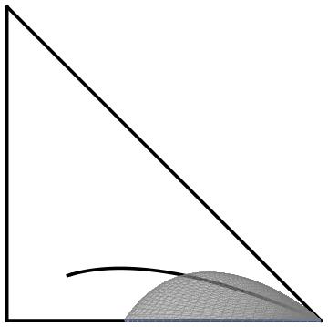 Figure 1
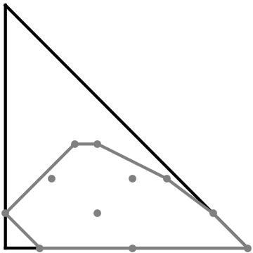 Figure 2
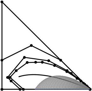 Figure 3
Peer Reviews
No public reviews on file for this paper yet. If you reviewed it on a platform where reviews are public (OpenReview, ICLR, NeurIPS, ICML), you can paste yours below so the community can read it here.
Videos
No videos yet. Explain this paper in a talk, walkthrough, or lecture? Add one.
Taxonomy
TopicsBayesian Methods and Mixture Models · Bayesian Modeling and Causal Inference · Markov Chains and Monte Carlo Methods
Exchangeable and Sampling Consistent Distributions on Rooted Binary Trees
Benjamin Hollering and Seth Sullivant
Abstract.
We introduce a notion of finite sampling consistency for phylogenetic trees and show that the set of finitely sampling consistent and exchangeable distributions on leaf phylogenetic trees is a polytope. We use this polytope to show that the set of all exchangeable and infinite sampling consistent distributions on 4 leaf phylogenetic trees is exactly Aldous’ beta-splitting model and give a description of some of the vertices for the polytope of distributions on 5 leaves. We also introduce a new semialgebraic set of exchangeable and sampling consistent models we call the multinomial model and use it to characterize the set of exchangeable and sampling consistent distributions.
1. Introduction
Leaf-labelled binary trees, which are commonly called phylogenetic trees, are frequently used to represent the evolutionary relationships between species. In this paper we will restrict our attention to rooted binary trees and our label set for a tree with leaves will always be and call such trees -trees, the set of which we denote .
Processes for generating random -trees play an important role in phylogenetics. Two common examples are the uniform distribution (where a tree is chosen uniformly at random from among all trees in ) and the Yule-Harding distribution (a simple Markov branching process). Some other examples of random tree models include Aldous’ -splitting model [1], the -splitting model [8], and the coalescent process (which generates trees with edge lengths) [16]. Two features common to all these random tree processes and desirable for any such tree process is that they are exchangeable and sampling consistent.
Let denote a probability distribution on . Exchangeability refers to the fact that relabeling the leaves of the tree does not change its probability. That is, for all and , . Exchangeability is a natural condition since it does not allow the names of the species to play any special role in the probability distribution. A family of distributions, , on trees has sampling consistency if for each , the distribution , which is on -trees, can be realized as the marginalization of distributions , which is on -trees, for . That is the probability of a -tree, , under can be written as
[TABLE]
Sampling consistency is a natural condition for a random tree model because it means that randomly missing species do not affect the underlying distribution on the species that were observed.
The goal of this paper is to study the structure of finitely sampling consistent distributions on rooted binary trees. In particular, we aim to obtain a finite deFinetti-type theorem for these trees in the style of Diaconis’ Theorem 4 in [6]. Our motivation is two-fold. First of all, there has been significant work on understanding the set of exchangeable, sampling consistent distributions on other discrete objects, including rooted trees. A classic result in this theory is deFinetti’s Theorem for infinitely exchangeable sequences of binary random variables which shows that every subsequence of the infinite sequence can be expressed as a mixture of independent and identically distributed sequences. This does not hold for finitely exchangeable sequences but Diaconis later developed a finite form of deFinetti’s theorem. He showed that if a finite exchangeable sequence of binary random variables, , can be extended to an exchangeable sequence, where , then the original sequence can be approximated with a mixture of independent and identically distributed sequences with error [6]. A substantial amount of work has been done on exchangeable arrays (see [7] for example) as well, which has been used to prove deFinetti theorems for other discrete objects. For instance, Lauritzen, Rinaldo, and Sadeghi recently developed a deFinetti Theorem for exchangeable random networks [12].
As previously mentioned, there has already been considerable work characterizing exchangeable and sampling consistent distributions on trees using weighted real trees as limit objects in [9, 10, 11]. In [11] a characterization of the exchangeable and sampling consistent Markov branching models we discuss in Section 3.1 is obtained. A true deFinetti theorem for trees is conjectured in [10] and proven in Theorem 3 of [9]. The approach taken in these papers is to characterize all infinitely sampling consistent distributions on trees using a tree-limit like object called a weighted real tree. In this paper, we instead take a geometric and combinatorial approach to the study of exchangeable and finitely sampling consistent distributions on binary trees and examine what happens as we take the limit.
A second motivation comes from the combinatorial phylogenetics problem of studying properties of the distribution of the maximum agreement subtree of pairs of random trees. Let and . The restriction tree is the rooted binary tree with leaf label set obtained by removing all leaves of not in and suppressing all vertices of degree 2 except the root. Two trees, , agree on a set if . A maximum agreement set is an agreement set of the largest size for and . The size of a maximum agreement subtree of these two trees is the cardinality of the largest subset that and agree on and is denoted . If is an agreement set with then the resulting tree is a maximum agreement subtree of and .
Understanding the distribution of for random tree distributions would help in conducting hypothesis tests that the similarity between the trees is no greater than the similarity between random trees. For example, it was suggested in [5] that could be used to test the hypothesis that no cospeciation occurred between a family of host species and a family of parasite species that prey on them. The study of the distribution of for random trees is primarily conducted with the assumption that and are drawn from an exchangeable, sampling consistent distribution on rooted binary trees. Bryant, Mackenzie, and Steel began the study of the distribution of and obtained some first bounds on for random trees and drawn from the Uniform or Yule-Harding distributions [3]. Later work on the distribution obtained an upper bound on the order of for when and are drawn from any exchangeable, sampling consistent distribution [2]. A lower bound on the order of has been conjectured for all exchangeable, sampling consistent distributions as well but this remains an open problem. Our hope in pursuing this project is that developing a better understanding of the set of all exchangeable sampling consistent distributions might shed light on this conjecture.
In this paper we study the structure of exchangeable, sampling consistent distributions on leaf labelled, rooted binary trees. We introduce a notion of a polytope of exchangeable and finitely sampling consistent distributions. We use it to study the set of exchangeable and sampling consistent distributions on trees and get some characterizations for trees with a small number of leaves. We show that set of all exchangeable and sampling consistent distributions on four leaf trees come from the -splitting model that was first introduced by Aldous in [1]. We have not been able to find a similar characterization for exchangeable and sampling consistent distributions on five leaf trees but we describe some of the vertices of the polytope of exchangeable and finitely sampling consistent distributions. We also introduce a new exchangeable and sampling consistent model on trees, called the multinomial model, and show that every sampling consistent and exchangeable distribution can be realized as a convex combination of limits of sequences of multinomial distributions.
2. Exchangeability and Finite Sampling Consistency
In this section we describe how the set of exchangeable distributions relates to the set of all distributions on leaf labelled, rooted binary trees. We then introduce a notion of finite sampling consistency and discuss how it relates to traditional sampling consistency.
Recall that denotes the set of all leaf labelled, rooted binary trees with label set , which we call -trees, and that . The set of all distributions on is the probability simplex where the coordinates are indexed by -trees. The symmetric group denotes the group of permutations of . For each and let denote the tree obtained by applying to the leaf labels.
Definition 2.1**.**
A distribution on is exchangeable if for all permutations and -trees , . The set of all exchangeable distributions on is denoted .
As previously mentioned, exchangeability requires that the probability of a -tree under a particular distribution depend only on the shape of the tree. Thus we only need to consider distributions on the set of tree shapes. Let denote the set of unlabelled rooted binary trees, which we may also call trees or tree shapes. This idea is summarized in the next lemma which is the -tree analogue of Lemma 2 in [12].
Lemma 2.2**.**
The set of exchangeable distributions on , , is a simplex of dimension with coordinates indexed by tree shapes.
Proof.
First we define a distribution for each tree shape . To do so, we let be the set of trees such that . For any tree we set
[TABLE]
Then since it is a probability distribution on trees and all trees of the same shape have the same probability. We claim that , where denotes the convex hull of the set . Since for all , it is enough to show that any distribution can be written as a convex combination of the . If , then the probability of any tree depends only on the shape of not the leaf labelling so we can write
[TABLE]
where represents the probability of any -tree in with shape . Since the original is a probability distribution on all leaf labelled trees the weights in the linear combination are nonnegative and sum to .
Lastly we note that the vectors are affinely independent since there is no overlap of coordinate indices where the entries in are nonzero. So is a simplex and has coordinates indexed by . ∎
Lemma 2.2 allows us to move from studying exchangeable distributions on leaf labelled -trees to all distributions on unlabelled trees. We will primarily focus on understanding the set of sampling consistent distributions within now. First recall that for the marginalization or projection map , gives a new distribution on for , defined for all by
[TABLE]
We will use this marginalization map to define a notion of finite sampling consistency.
Definition 2.3**.**
A family of distributions is finitely sampling consistent or -sampling consistent, if for each , . We denote the set of all distributions in that are -sampling consistent by
[TABLE]
It is immediate that if a distribution in is -sampling consistent, then for any , such that , the distribution is also -sampling consistent. This leads to the following:
Lemma 2.4**.**
For all ,
[TABLE]
A distribution in , is sampling consistent if it is part of a -sampling consistent family of distributions for all . In other words, a distribution is sampling consistent if it is in for all . Thus we can define the following notation for the set of exchangeable distributions on that are sampling consistent:
[TABLE]
Lemma 2.5**.**
Let be defined as it is in Lemma 2.2, then
[TABLE]
Proof.
Clearly it holds that since for all . It is enough to show that if we have a distribution , then it can be written as a convex combination of the . If , then there exists such that . Since , we know from Lemma 2.2 that we can write . Then evaluating at a -tree gives
[TABLE]
Changing the order of summation we have
[TABLE]
but so we get that
[TABLE]
which shows that can be written as a convex combination of the . ∎
Example 2.6**.**
While it will be the case that , not every will be a vertex of . Figure 1 illustrates this.
Lemma 2.5 implies that understanding how the marginalization map acts on the vertices of will allow us to compute all of . The following lemma and corollary will give us a method for calculating the vertices of by computing subtree densities.
Lemma 2.7**.**
Let and . Also let . Then .
Proof.
By definition of the map
[TABLE]
but is nonzero if and only if , in which case it is . So the above sum becomes
[TABLE]
∎
Corollary 2.8**.**
Let and . Then , which is used to denote the sum of over all , is the induced subtree density of in . That is, is the ratio of the number of times that occurs as a restriction tree of when of its leaves are marginalized out.
Proof.
From the previous lemma, we know that for any , where . Then we have
[TABLE]
So for each labelling of , we are counting which fraction of labellings of yield when restricted to . As we sum over all labellings of , this gives us the total fraction of times that the shape appears as a restriction tree of the shape when of its leaves are marginalized out. ∎
The following examples elucidates what is meant by induced subtree density and shows how we can explicitly calculate this quantity.
Example 2.9**.**
We show how to find the projection of one vertex of down to . is the convex hull of the projection of all of the vertices of . Begin with the tree shape pictured in Figure 2(a). We label the leaves of for the sake of the calculation but it should be thought of as an unlabelled tree. We then find the shape of the restriction tree for the five -subsets of . The restriction of to the leaf sets , gives the shape and the restriction to the sets gives the shape , pictured in Figure 2(b). We let the first coordinate of be the probability of obtaining and the second be the probability of obtaining . As mentioned above, these probabilities will simply be the number of times each shape appears as a restriction tree over the total number of restriction trees. Thus this vertex of will give us the distribution in .
We have now seen how to compute the vertices of explicitly but not every distribution is a vertex of . However, the comb tree always yields a vertex of .
Lemma 2.10**.**
For all , let be the -leaf comb tree, then is a vertex in .
Proof.
The comb tree has only smaller comb trees as restriction trees, so the image of the comb distribution on leaves under the marginalization map will be the comb distribution on leaves. Since is a vertex of and is a subset of , then is also a vertex of . ∎
3. Examples of Exchangeable and Sampling Consistent distributions
In this section we discuss some of the well-known exchangeable and sampling consistent families of distributions particularly, the Markov branching models. We also introduce a new family of exchangeable sampling consistent tree distributions, namely the multinomial family.
3.1. Markov Branching Models
An important example of sampling consistent and exchangeable distributions are the families of Markov branching models which can be constructed in the following way as first introduced in [1] by Aldous.
Suppose that for every integer , we have a probability distribution on which satisfies . Using this family of distributions we can define a probability distribution on by taking the probability that leaves fall on the left of the root-split and leaves fall on the right of the root-split to be with each choice of labels to fall on the left having the same probability. Repeating recursively in each branch will yield the probability of a rooted binary tree. Aldous called these models Markov branching models.
Haas et al. classified the sampling consistent Markov branching models on rooted binary trees in [11]. They show that every sampling consistent Markov branching model, defined by the splitting rules , , has an integral representation of the form
[TABLE]
where , is a symmetric measure on such that , and is a normalization constant. accounts for the comb distribution. A subclass of these models are those where the measure in equation (1) has the form for a probability density function on that is symmetric on the interval (i.e. ) and where . These Markov branching models can be thought of as uniformly choosing points in the interval at random and then splitting the interval with respect to the density . Repeating the splitting process recursively in each subinterval until each of the original points is contained in its own subinterval gives a tree shape. This process is pictured in Figure 6 in [1].
One particularly important family of Markov branching distributions is the beta-splitting model. It is a Markov branching model that belongs to the subclass mentioned above where the function in the above description has the form
[TABLE]
for . For the beta-splitting model we can calculate the values explicitly in terms of . By plugging in the beta-splitting density function into (1) for we get the following formulas:
[TABLE]
for . Note that (2) gives a valid probability distribution when and so it is natural to extend the beta-splitting model to those values of , although the density is not well-defined in that case. As approaches the beta-splitting model approaches the distribution which puts all probability on the comb tree, so we also include in the beta splitting model as the comb distribution.
An important note here is that for the beta-splitting model each is actually a rational function in . Using properties of the gamma function one can see that the above formula simplifies to
[TABLE]
Since each is a rational function in , we can see that the probability of obtaining a certain tree shape is a rational function in as well because the probability of obtaining that tree shape under the beta-splitting model is simply the product of the probability of all of the splits in the tree.
Example 3.1**.**
Let and be the trees pictured in Figure 2(b). Then the probabilities of obtaining them under the beta-splitting model are
[TABLE]
This model also has a nice characterization among all of the sampling consistent Markov branching models. In [14], Mccullagh, Pitman, and Winkel show that the beta-splitting models are the only sampling consistent Markov branching models whose splitting rules admit a particular factorization.
We are interested in examining how the sampling consistent Markov branching models and in particular the beta-splitting model fits inside inside of as a whole. These distributions are infinitely sampling consistent and so lie in as well. A priori, it might seem that to determine the probability of a tree shape with leaves under a Markov branching model that one would need to have not only the distribution but also distributions where . This is actually not the case for any sampling consistent Markov branching model though. Ford showed in Proposition 41 of [8] that if are the splitting rules for a distribution in , then in fact it must be that
[TABLE]
This implies that all that is needed to define a distribution in is the first splitting rule which gives the following corollary.
Corollary 3.2**.**
The dimension of the set of all sampling consistent Markov branching models in is at most
Proof.
As explained above, a Markov branching model is completely determined by the distribution which determines all of the distributions where . Since must be symmetric we immediately get that the values determine all of . Also since must be a distribution we lose one of these as a free parameter, thus the dimension of the set of sampling consistent Markov branching models is bounded above by . ∎
Note that when , the space of sampling consistent Markov branching models has dimension . We will see in Section 4 that the set of beta-splitting models is equal to the set of sampling consistent Markov branching models in this case.
3.2. Multinomial model
The multinomial model is a model that associated to each tree shape for any a family of probability distributions on for each . We will often extend the model to allow to use extended trees with an additional leaf added to the root. We associate to every edge, , in a parameter . This gives us a vector of parameters of length , and we assume that , so that these parameters give a probability distribution on the edges of . We will now use this probability distribution to define a set of distributions on for any . Note that and do not have to be related to each other.
Using the distribution , we draw a multiset of edges from the tree , where edge occurs with probability . There is a natural way to take the tree and a multiset of size on the set of parameters and construct a new tree which we will call . Each time that an edge appears in , we add a new leaf to the edge , which will give us a new tree with an undetermined number of leaves. We then simply take to be the induced subtree on only the leaves that come from . Hence, the multinomial model on the tree gives a way to produce random trees with an underlying skeleton that is the tree . For large , the resulting random trees look like with many extra leaves added.
The multinomial probability of observing a particular multiset of edges is the monomial
[TABLE]
where denotes the number of times that appears in the multiset , and is the resulting vector.
Letting be the set of all element multisets of edges of , we can calculate the probability of observing any particular tree shape by
[TABLE]
Example 3.3**.**
Consider the tree from Figure 3(b) with edge parameters . To calculate the probability of the tree, , in Figure 3(c) we use the formula
[TABLE]
The only multisets that satisfy this condition are the sets and . This is because if appears in a multiset any positive number of times, the tree will have a single leaf on one side of the root and four leaves on the other side, regardless of what other parameters appear in the set. So and are the only elements of that we sum over so
[TABLE]
The multinomial model gives a family of distributions as we let the parameter vector range over the entire simplex. Equivalently, the model can be described as the image of the simplex under the polynomial map
[TABLE]
where the coordinate corresponding to has value for . Since is a semialgebraic set and is a polynomial map, the multinomial model is also a semialgebraic set.
It also holds that if we take any tree , and any subtree of , then we have that . This is because if the parameters corresponding to edges that appear in but not in are set to [math] in , the map will simply become . Setting these parameters to [math] just corresponds to restricting to a subset of the simplex and thus we get the image containment.
A last interesting note is that this model is perhaps similar in spirit to the -random graphs when is a graphon obtained from a finite graph as described in [13]. The construction begins with a finite graph and uses it to define a distribution on graphs with vertices similarly to how we begin with a tree and define a distribution on trees with leaves.
We end this section with Figure 4, which shows both the beta-splitting model and the multinomial model inside . In the next section we will discuss the exchangeable and sampling consistent distributions on four leaf trees and how they relate to the models discussed in this section.
4. Distributions in
In this section we classify all of the distributions in . In particular, we show that is equal to the beta-splitting model.
First we note that since there are only two distinct tree shapes with four leaves (see Figure 3(a)), the set of exchangeable distributions is just a 1-dimensional simplex in . We take coordinates on and let the first coordinate correspond to and the second coordinate to . The subset of distributions that are also sampling consistent must be some line segment within the simplex. We know from Lemma 2.10 that the comb distribution, which is in these coordinates, is a vertex in . If we can bound the probability of obtaining then we will have a complete characterization of all distributions in . Theorem 14 in [4] will be the main tool to achieve this.
Theorem 4.1**.**
[4, Thm 14]** The most balanced tree in has the complete symmetric tree on four leaves appear more frequently as a subtree than any other tree in .
By the most balanced tree in , we mean the unique tree shape in that has the property that for any internal vertex of the tree, the number of leaves on the left and right subtrees below that differ by at most one.
Theorem 4.2**.**
The four leaf beta-splitting model equals the set of all exchangeable and sampling consistent distributions on .
Proof.
Note that only has two vertices since it is a line segment. The comb distribution is always a vertex in , by Lemma 2.10. The other vertex will be the projection of the vertex of that places the most mass on . The projection of a vertex , is where is the number of element subsets such that and is the number of element subsets such that . By Theorem 4.1 we can restrict to the most balanced tree in . We will use to denote this highest value of that we get from the most balanced tree in .
The beta-splitting model on , on the other hand, is the line segment from to . Indeed, under the beta splitting model, the probability of is just
[TABLE]
As , this converges to . So if we can show that then we will be done.
To prove that , we can restrict to the subsequence of values , since Lemma 2.4 implies that is a monotone decreasing sequence. This subsequence is easier to deal with since counts the number of -subsets, of the leaves of the complete symmetric tree in such that . It is not hard to come up with a simple recurrence for this though since has the recursive structure as illustrated in Figure 5.
Note that since the only ways we can choose a subset such that are that the leaves in fall either entirely within the left or right subtrees or that has two leaves from both the left and right subtrees. The number of ways to choose a subset that falls entirely on the left or right side is by definition. The number of ways to choose two leaves from each side is . This recurrence can be solved to find an explicit formula for which is
[TABLE]
Now we can simplify to get
[TABLE]
which converges to as tends to infinity. ∎
Note that Theorem 4.2 does not generalize to higher dimensions as the set of beta splitting distributions is of strictly smaller dimension than the set of exchangeable sampling consistent distributions. We explore the discrepancy between these sets in more detail in the next sections.
5. Distributions on
There are three distinct tree shapes with five leaves so is a -dimensional simplex in . For the rest of this section we will use , , and to represent the trees pictured in Figure 6. Specifically, let denote the comb tree on five leaves, denote the balanced tree on five leaves and denote the giraffe tree on five leaves. We take coordinates on where represent the probability of obtaining , , and , respectively.
While have not been able to give a complete description of the vertices of for all , we are able to define some tree structures in that do yield vertices of . We have already seen that the comb tree always yields a vertex of for all and . Here we provide some other examples.
Definition 5.1**.**
For a tree let be the tree that is obtained by creating a comb tree with leaves and replacing one of the two leaves at the deepest level with the tree .
Generally, if then has vertices. For example, . Note that does not matter which of the leaves is replaced with since our trees are unlabelled.
Proposition 5.2**.**
Let . Then is a vertex in .
Proof.
First note that and are the only trees with leaves that do not have as a subtree. This means that and the comb tree fall on the line in . Thus, the set is a face of for all , since every distribution must satisfy the condition and thus . Since is the same line as it defines a face. Now since and are different points are the only distributions of the form in this face, they must be vertices of this face and thus vertices of . ∎
We now introduce another tree structure that will yield a vertex in .
Definition 5.3**.**
For two positive integers and let denote the tree made by joining a comb tree of size and a comb tree of size together at a new root. We call such trees bicomb trees.
For example, .
Lemma 5.4**.**
Let . Then is a vertex of .
Proof.
First note that for , the only trees in that never contain as a restriction tree are the comb tree and the bicomb trees. This means that in , they are the only trees that fall on the edge . To show that is a vertex of it remains to to show that is extremal on this edge. We know that the comb tree is one of the extremal points on this edge and so the other extremal point will correspond to the bicomb tree with the highest density of as a restriction tree. Let be a bicomb tree for some . We let denote the number of times that occurs as a restriction tree of . From the structure of a bicomb tree we have
[TABLE]
This function is maximized when . ∎
Now we will show that the projection of the most balanced tree in is a vertex of . To do this, we prove a few lemmas about the number of trees that can appear as subtrees of a tree. These results follow the basic outline of Lemmas 12 and 13 in [4], and are in some sense an extension of those results to leaf trees.
For a tree let count the number of -subsets, , of the leaves of such that . Let be defined similarly, but for leaf comb trees.
Lemma 5.5**.**
Let be as it is pictured in Figure 7 and obtained from by swapping the positions of and . For , let and without loss of generality choose and . If and then . Furthermore, if , then .
Proof.
Without loss of generality assume that and and let denote the set of leaves of below the vertex . Note that by construction, this is the same as the set of leaves below the vertex in . If we take a -subset, , of the leaves of and then it is only possible for if . It is straightforward to see that if has zero, one, two, or three elements, .
This means
[TABLE]
where and denote the subtrees of and below . Note that for any tree , it holds that
[TABLE]
which gives
[TABLE]
and is guaranteed to be positive by Lemma 12 of [4] so the term is nonnegative. It remains to show that is nonnegative. We can explicitly enumerate these quantities in the following way:
[TABLE]
[TABLE]
We can simplify this to get that
[TABLE]
Note that this quantity is greater than [math] since and by assumption and for . Note that if , then we either have that , or which both guarantee that . ∎
This lemma essentially tells us that if the tree has an internal node that is unbalanced, we can find a tree that has appear less frequently as a restriction tree. We now have another lemma following in the style of [4].
Lemma 5.6**.**
Let be as it is pictured in Figure 8 and for , let and assume . We also assume that . Then . Furthermore, if , then .
Proof.
We will again proceed by showing that . By the same reasoning as that given in the last lemma we know that
[TABLE]
and the nonnegativity of the second term follows in the same manner that was described in the previous lemma. Now we can easily see that
[TABLE]
[TABLE]
and so
[TABLE]
It is clear that the right hand side is always nonnegative. Note that if , then either or . In both cases this guarantees that .
∎
Combining these two lemmas together we get the following theorem. This theorem will immediately allow us to show that the projection of the most balanced tree in will always be a vertex in .
Theorem 5.7**.**
For , the minimum value of is attained when every internal node of is maximally balanced.
Proof.
This proof also follows the strategy of [4]. We assume that obtains it minimum value in at but that is not maximally balanced. We will try to find a contradiction. We let be a non-balanced internal node with balanced children and . We let and be the number of leaves of the trees rooted at and respectively. Then since is not balanced we have, without loss of generality, that . If is a leaf then by Lemma 5.6 we immediately have that is not minimum since . So we have that and thus both and are balanced and must be internal nodes.
We now let be the children of and be the children of and take for and once again without loss of generality assume that and . Since both and are balanced it must be that or and or . Then the assumption that immediately gives us that
[TABLE]
Then by previous assumptions we get that . Now since is minimum at and , we can apply Lemma 5.5 to get that . Stringing together these inequalities we get that
[TABLE]
But since or , the only possibility we have is that
[TABLE]
But then we get that and which contradicts the inequality . This tells us that any tree with at least leaves must be maximally balanced around every internal node if it obtains the minimum value of on . Since there is only one tree that is maximally balanced at every internal node, there is a unique minimizer of in for . ∎
Corollary 5.8**.**
Let be the maximally balanced tree in . Then is a vertex of .
Proof.
The Corollary can be verified computationally for . For Theorem 5.7 shows that is the unique tree that attains the minimum value of among all trees in . So it holds that , thus is a vertex of . ∎
We have another Corollary that relates the exchangeable and sampling consistent distributions to the -splitting model.
Corollary 5.9**.**
The projection of the most balanced tree in approaches the point on the beta-splitting model as .
Proof.
It is enough to show that the complete symmetric tree satisfies this property. We can just count the number of times that and occur as restriction trees when we restrict to a 5-subset of the leaves. We will call these quantities and respectively. Once again since has the structure depicted in Figure 5 and we can use this structure to write down a simple recurrence for and and then solve the recurrence. Since we can either choose our subset to be on either the right or left side of the tree or 3 leaves from one side and 2 leaves from the other, is simply
[TABLE]
As for , we can once again choose our subset to be on either the right or left side of the tree or we can choose to have 1 leaf on a side of the tree and a 4 leaf symmetric tree on the other. This can be done in just ways. So is just
[TABLE]
Both of these recurrences can be solved explicitly using a computer algebra system. We get that
[TABLE]
[TABLE]
We can then find the probabilities and of and by simply dividing out by . This yields
[TABLE]
[TABLE]
Clearly as we have and .
On the other hand, we recall that the probability of obtaining a tree under the beta-splitting model is just a rational function in that can be explicitly calculated. We can then find the limit of these rational functions to get that the beta-splitting curve approaches the point
[TABLE]
as as well and so the projection of in is approaching the point on the curve. ∎
These are all of the tree structures in we have been able to find that always appear as vertices in . We end this section with Figure 9, which pictures all of the families of exchangeable and sampling consistent distributions that we have discussed and the vertices of for some small values of .
6. Distributions on
While we are not able to get a description of the vertices of for general and , it is possible to to describe using the multinomial model that was introduced in Section 3.2. In particular, this shows that multinomial models converge as an inner limit to .
Theorem 6.1**.**
Let be a sequence of tree shapes and be the corresponding sequence of distributions. If converges to some as goes to infinity, then there exists a sequence of multinomial distributions that also converges to as goes to infinity.
Proof.
Define to be the multinomial distribution on the tree with the edge parameter vector such that if one of the vertices in is one of the original leaves of and otherwise. Note that these nonzero edge parameters are bijectively associated to the leaves of and we may call the set of nonzero edge parameters meaning the leaf set of . To show that also converges to , it is enough to show that for every tree , . Fix a labelling of and let be the number of sets such that . By Corollary 2.8, is the induced subtree density of in , so . So
[TABLE]
On the other hand, let , then
[TABLE]
by definition and we note by requiring that multisets have that , only includes multisets whose support is contained in . Also note that is either [math] or since all the edge parameters are [math] or . So to understand the quantity it is enough to know the coefficient of . Note that any multiset has a naturally associated integer partition of to it, formed by taking the multiplicities of each unique element that appears in it. Call this integer partition the weight of , denoted , and let be the set of multisets in with weight . Now observe that for , since the value of the multinomial coefficient is totally determined by the weight and the product of the edge parameters is always . If we let be the value of the multinomial coefficient then the formula for can be rewritten as
[TABLE]
but we can bound the quantity . We note that the quantity , of all multisets on the edge parameters of of size, with weight , is at most where is the length of the partition . This is because there are choices for which elements to use in the multiset and at most unique multisets for each choice of elements. Since is a polynomial in of degree though, we have that
[TABLE]
since the partition is the only partition where is of the order , and so is the only term that contributes to the limit. Now we note that the multisets correspond exactly to choosing subsets of the leaves of that yield upon restriction since the only edges that can be in are those corresponding to leaves, every leaf can be chosen at most once, and . So , and so
[TABLE]
and since converges, to , it must be that also does. ∎
Corollary 6.2**.**
Suppose that for some . Then for any tree , can be approximated with a distribution with error , where is a constant with respect to that does not depend on the tree .
Proof.
Note that if , then we have for every ,
[TABLE]
where the above combination is convex by Lemma 2.5. Then let be defined as the multinomial distribution on just as is defined for in the previous theorem. Then recall from the proof of the previous theorem that
[TABLE]
where . Also recall from the proof of the previous theorem that . Combining these facts with the definition of and the triangle inequality gives
[TABLE]
and we now bound each term on the right hand side of this inequality.
To bound the first term in equation (4), note that is a nonnegative quantity and is bounded above by . This gives the inequality
[TABLE]
where is a constant. Note that this constant does not depend on the trees and .
To bound the second term we again recall from the proof of the previous theorem that for each partition of . Then we have that
[TABLE]
but since , it must be that so for all the remaining partitions . Applying this fact to the right hand side of equation (6) gives the bound
[TABLE]
where is a constant that also does not depend on the trees and . Applying the bounds for each term to equation (4) and setting gives
[TABLE]
and again we note that is independent of the trees and since and are. We are now ready to construct a distribution that gives the desired result. From the discussion of the multinomial model, we have that each distribution and so from the convexity of we get
[TABLE]
We can now use the expression for we began with and the bound obtained in equation (8) to get that
[TABLE]
∎
Theorem 6.1 gives that the limit of any convergent sequence where can also be realized as the limit of points coming from multinomial models. Corollary 6.2 shows that if we have a distribution in that can be extended to part of a finitely sampling consistent family, then it can be approximated with an infinitely sampling consistent distribution. With Theorem 6.1 and the following theorem, we will show that is actually the convex hull of all limits of convergent sequences of vertices, and thus the convex hull of limits of distributions drawn from the multinomial model. To do this we need a basic proposition from convex analysis which the proof of is included for completeness.
Proposition 6.3**.**
Let be a sequence of polytopes in such that for all , . Let
[TABLE]
where the bar denotes the closure in the Euclidean topology. Then .
Proof.
It is straightforward to see that . To show that the sets are equal suppose that there is . Then the Basic Separation Theorem of convex analysis implies there must exist an affine functional with and for all . We also have that since , for each , can be written as
[TABLE]
where the are the vertices of . Then because it must be that for each , there exists at least one vertex of such that . Since all the points lie in which is a compact set, there exists a convergent subsequence with limit , thus . But it also holds that
[TABLE]
which is a contradiction. ∎
Corollary 6.4**.**
Let denote the specific multinomial model construction on the tree described in Theorem 6.1. Then
[TABLE]
Proof.
Recall that , thus by Proposition 6.3,
[TABLE]
since the vertices of correspond to a subset of the points . Applying Theorem 6.1 to the sequence gives the result. ∎
Corollary 6.4 shows that every exchangeable and infinitely sampling consistent distribution is either a convex combinations of limits of multinomial distributions or a limit point of points in that set. Understanding the structure of the multinomial models may shed greater light on the structure of as a whole. We view Corollary 6.2 and Corollary 6.4 as the rooted binary tree analogue to Theorems 3 and 4 in [6], in essence they are finite forms of a deFinetti-type theorem for rooted binary trees. As previously mentioned, the work done in [10] and [9] establishes a more typical deFinetti theorem in the sense that it shows every infinitely sampling consistent sequence of distributions can be obtained by sampling from a limit object using techniques from Probability theory.
We also note that the requirement that the induced subtree densities converge is quite similar to the idea of graph convergence that appears in [13] and that many of the ideas in the theory of graph limits may also be applied to trees. The very well developed theory of graph limits contains many equivalent versions of the limiting object (see Theorem 11.52 in [13]). The work done in [10] and [9] makes the connection between the limiting object,a random real tree, and an infinitely sampling consistent model. It is still unknown if this can be connected to ideas such as tree parameters (the induced subtree density for instance) and to metrics on finite trees as has been done in the theory of graph limits. It seems that many of these equivalences hold but differences in techniques will be required.
Acknowledgments
Benjamin Hollering and Seth Sullivant were partially supported by the US National Science Foundation (DMS 1615660). Thanks to Dávid Papp for a helpful conversation regarding Proposition 6.3.
The reference list from the paper itself. Each links out to its DOI / PubMed record.
- 1[1] David Aldous. Probability distributions on cladograms. In Random discrete structures (Minneapolis, MN, 1993) , volume 76 of IMA Vol. Math. Appl. , pages 1–18. Springer, New York, 1996.
- 2[2] Daniel Irving Bernstein, Lam Si Tung Ho, Colby Long, Mike Steel, Katherine St. John, and Seth Sullivant. Bounds on the expected size of the maximum agreement subtree. SIAM J. Discrete Math. , 29(4):2065–2074, 2015.
- 3[3] David Bryant, Andy Mc Kenzie, and Mike Steel. The size of a maximum agreement subtree for random binary trees. In Bioconsensus (Piscataway, NJ, 2000/2001) , volume 61 of DIMACS Ser. Discrete Math. Theoret. Comput. Sci. , pages 55–65. Amer. Math. Soc., Providence, RI, 2003.
- 4[4] T. M. Coronado, A. Mir, F. Rosselló, and G. Valiente. A balance index for phylogenetic trees based on quartets. Ar Xiv e-prints , March 2018.
- 5[5] D. M. de Vienne, T. Giraud, and O.C. Martin. A congruence index for testing topological similarity between trees. Bioinformatics , 23:3119–3124, 2007.
- 6[6] Persi Diaconis. Finite forms of de finetti’s theorem on exchangeability. Synthese , 36(2):271–281, Oct 1977.
- 7[7] Persi Diaconis and Svante Janson. Graph limits and exchangeable random graphs. Rend. Mat. Appl. (7) , 28(1):33–61, 2008.
- 8[8] Daniel J. Ford. Probabilities on cladograms: Introduction to the alpha model . Pro Quest LLC, Ann Arbor, MI, 2006. Thesis (Ph.D.)–Stanford University.