Quasi-optimal and pressure robust discretizations of the Stokes equations by new augmented Lagrangian formulations
Christian Kreuzer, Pietro Zanotti

TL;DR
This paper introduces new discretization methods for the stationary Stokes equations that are quasi-optimal and pressure robust, using augmented Lagrangian formulations to improve accuracy without requiring divergence-free finite element pairs.
Contribution
The paper develops a novel augmented Lagrangian approach that achieves pressure robustness and quasi-optimality for various finite element pairs in Stokes discretizations, without divergence-free constraints.
Findings
Velocity error proportional to best approximation error
Pressure error bounded by approximation errors
Applicable to conforming and nonconforming finite element pairs
Abstract
We approximate the solution of the stationary Stokes equations with various conforming and nonconforming inf-sup stable pairs of finite element spaces on simplicial meshes. Based on each pair, we design a discretization that is quasi-optimal and pressure robust, in the sense that the velocity -error is proportional to the best -error to the analytical velocity. This shows that such a property can be achieved without using conforming and divergence-free pairs. We bound also the pressure -error, only in terms of the best approximation errors to the analytical velocity and the analytical pressure. Our construction can be summarized as follows. First, a linear operator acts on discrete velocity test functions, before the application of the load functional, and maps the discrete kernel into the analytical one. Second, in order to enforce consistency, we employ a new augmented…
Click any figure to enlarge with its caption.
 Figure 1
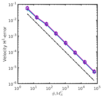 Figure 2
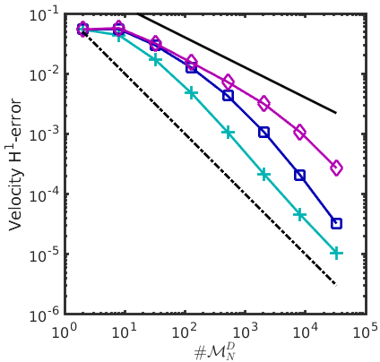 Figure 3
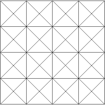 Figure 4
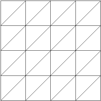 Figure 5
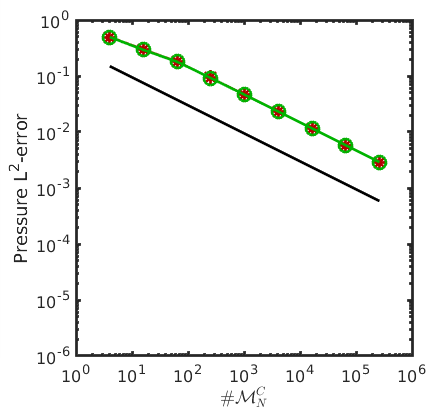 Figure 6
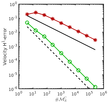 Figure 7
| N | -error EOC | -error EOC |
|---|---|---|
| 4 | 3.32e-04 | 3.32e-04 |
| 5 | 8.31e-05 1.00 | 8.31e-05 1.00 |
| 6 | 2.08e-05 1.00 | 2.08e-05 1.00 |
| 7 | 5.19e-06 1.00 | 5.19e-06 1.00 |
| 8 | 1.30e-06 1.00 | 1.30e-06 1.00 |
Peer Reviews
No public reviews on file for this paper yet. If you reviewed it on a platform where reviews are public (OpenReview, ICLR, NeurIPS, ICML), you can paste yours below so the community can read it here.
Videos
No videos yet. Explain this paper in a talk, walkthrough, or lecture? Add one.
Quasi-optimal and pressure robust
discretizations of the Stokes equations by
new augmented Lagrangian formulations
Christian Kreuzer
TU Dortmund
Fakultät für Mathematik
D-44221 Dortmund
Germany
and
Pietro Zanotti
TU Dortmund
Fakultät für Mathematik
D-44221 Dortmund
Germany
Abstract.
We approximate the solution of the stationary Stokes equations with various conforming and nonconforming inf-sup stable pairs of finite element spaces on simplicial meshes. Based on each pair, we design a discretization that is quasi-optimal and pressure robust, in the sense that the velocity -error is proportional to the best -error to the analytical velocity. This shows that such a property can be achieved without using conforming and divergence-free pairs. We bound also the pressure -error, only in terms of the best approximation errors to the analytical velocity and the analytical pressure. Our construction can be summarized as follows. First, a linear operator acts on discrete velocity test functions, before the application of the load functional, and maps the discrete kernel into the analytical one. Second, in order to enforce consistency, we employ a new augmented Lagrangian formulation, inspired by Discontinuous Galerkin methods.
1. Introduction
We consider the discretization of the stationary Stokes equations
[TABLE]
with viscosity , in a bounded domain , . According to the classical approach of Brezzi [12], we approximate the analytical velocity and the analytical pressure by means of discrete spaces and , which are required to fulfill the so-called inf-sup condition. We additionally assume that and are finite element spaces on a simplicial mesh of .
To motivate our work, let us focus on the velocity -error, i.e. the error between and the discrete velocity , measured in the -norm. We refer to [8, Chapter 5] for the proof of the results listed hereafter. The Céa’s-type quasi-optimal estimate
[TABLE]
is well-known for standard discretizations (see (2.2) and (2.11) below) with conforming and divergence-free pairs, i.e. under the assumptions and . Such pairs have attracted a growing interest in recent years; see [18, 19, 32, 37] and the references therein. Owing to (1.2), this class of discretizations seems particularly attractive, because it fully exploits, up to a constant, the approximation properties of the space in the -norm. This prevents, in particular, from the following issues.
For standard discretizations with general conforming pairs (see (2.2) and (2.5) below) one typically has
[TABLE]
Thus, if , the right-hand side suggests that the velocity -error may be not robust with respect to the pressure. This is indeed the case and such effect is known in the literature as poor mass conservation. It becomes extreme for purely irrotational loads or for small values of the viscosity; see, for instance, [24]. Poor mass conservation discourages, in particular, from the use of unbalanced pairs, i.e. pairs so that the approximation power of in the -norm is higher than the one of in the -norm; cf. Remark 3.1.
Recall also that, in the nonconforming case , estimates in the form
[TABLE]
are often derived. Here is an extension of the -norm to and the semi-norm is defined on (a subspace of) . Since the lack of smoothness in is commonly compensated by additional regularity of the load beyond , the semi-norm cannot be extended to and potentially dominates the right-hand side of (1.4) for rough solutions. Therefore, an estimate like (1.3) cannot be expected to hold, cf. Remark 2.3.
Several techniques are available in the literature to deal with the above mentioned difficulties. The discretization of [4, section 6] and the general framework in [33] indicate how to avoid the issue with for nonconforming pairs. The over-penalized augmented Lagrangian formulation of [10] and the grad-div stabilization [28] may serve to mitigate the impact of poor mass conservation. More recently, Linke et al. [23, 24, 25] proposed a class of discretizations, which differ from standard ones only in the treatment of the load and enjoy the following pressure robust upper bound
[TABLE]
for several conforming and nonconforming pairs.
In this paper, we show that the quasi-optimal and pressure robust estimate (1.2) is not a prerogative of conforming and divergence-free pairs, but can be achieved also by (carefully designed) discretizations, based on general inf-sup stable pairs. In this way, we combine the advantages of the various techniques listed above. We also bound the pressure -error only in terms of the best approximation errors to the analytical velocity and to the analytical pressure. To our best knowledge, similar error bounds were previously obtained only in [35] in the rather specific case of the lowest-order nonconforming Crouzeix-Raviart pair [14]. In particular, our results make unbalanced pairs a valuable option, if one is more interested in the analytical velocity rather than in the analytical pressure.
Our approach is guided by few simple necessary conditions and builds on two main ingredients. First, we discretise the load with the help of an operator which maps into and discretely divergence-free into exactly divergence-free functions. The importance of the latter property was first devised in [24]. For this purpose, we solve local Stokes problems with Scott-Vogelius elements on a barycentric refinement of the mesh, see [19, 30, 36]. Second, we discretise the weak form of the Laplace operator in a way inspired by Discontinuous Galerkin (DG) methods, in order to enforce the necessary consistency. The resulting discretization can be interpreted as a new augmented Lagrangian formulation, cf. Remark 3.7.
The rest of the paper is organized as follows. In section 2 we set up the abstract framework. In section 3 we illustrate our construction by means of a model example. Various generalizations are then discussed in section 4. Finally, in section 5 we complement our theoretical findings through some numerical experiments.
2. Abstract framework
This section introduces an abstract discretization of (1.1) and the properties in which we are interested. Two basic results are also proved. We use standard notations for Lebesgue and Sobolev spaces.
2.1. Quasi-optimal discretizations
Let , , be an open and bounded polytopic domain with Lipschitz-continuous boundary. The weak formulation of the stationary Stokes equations in , with viscosity and load , looks for and such that
[TABLE]
Here denotes the euclidean scalar product of tensors and is the dual pairing of and . Due to the boundary condition on the analytical velocity , the analytical pressure belongs to . Problem (2.1) is uniquely solvable, according to [8, Theorem 8.2.1].
Remark 2.1* (Alternative formulation).*
Most of our subsequent results remain unchanged in case the gradient is replaced by the symmetric gradient in the first equation of (2.1) and the homogeneous Neumann condition is imposed on (a portion of) . The only remarkable difference is that a piecewise Korn’s inequality may fail to hold for some of the nonconforming pairs mentioned in section 4.1, see [2, 11]. This problem, however, can be overcome e.g. by an additional jump penalization in the spirit of [34, Section 3.3].
We consider discretizations that mimic the variational structure of problem (2.1). More precisely, we approximate and in finite-dimensional linear spaces and . We require and measure the pressure error in the -norm . Instead, we allow for nonconforming discrete velocity spaces . In order to measure the velocity error, we assume that an extension of the -norm to is at our disposal. We replace the bilinear forms in (2.1) with discrete surrogates and . Moreover, we let be a linear operator. Hence, we look for a discrete velocity and a discrete pressure such that
[TABLE]
To ensure that this problem is uniquely solvable, we assume hereafter that is coercive on and that the pair is inf-sup stable, i.e.
[TABLE]
for some constant , see [8, Corollary 4.2.1]. Note, in particular, that the duality is well-defined for all and , also in the nonconforming case.
We shall pay special attention to the following property, which guarantees that is a near-best approximation of in .
Definition 2.2** (Quasi-optimality).**
Denote by and the solutions of (2.1) and (2.2), respectively, with load and viscosity . We say that (2.2) is a quasi-optimal discretization of (2.1) when there is a constant such that
[TABLE]
for all and . We denote by the smallest such constant.
According to [8, Theorem 5.2.5], the discretization (2.2) is quasi-optimal if
[TABLE]
i.e. if is a conforming pair and , and are simple restrictions of their conforming counterparts in (2.1). In sections 3 and 4 we show that quasi-optimality can be achieved also with nonconforming pairs and/or for different choices of and .
Remark 2.3* (Smoothing by ).*
Since is finite-dimensional, the operator is bounded and the solution of (2.2) depends continuously on the -norm of . This property, in turn, prevents the issue pointed out in the introduction concerning the semi-norm in (1.4). Of course, such observation is of practical interest only if the norm of is of moderate size, so that it does not affect too much the stability constant of (2.2). We call ”smoothing” operator, because it increases the smoothness of the elements of whenever . For conforming pairs, one can let be the identity as in (2.5). This choice is compatible with quasi-optimality but, possibly, it is not pressure robust; compare with section 2.2 below.
Remark 2.4* (Computational feasibility).*
It is highly desirable that there are bases and of and , respectively, such that the scalars
[TABLE]
can be computed or approximated, up to a prescribed tolerance, with operations, for all and . This ”computational feasibility” is not necessary for quasi-optimality but guarantees that the solution of (2.2) can be computed with optimal complexity.
2.2. Quasi-optimal and pressure robust discretizations
The analytical velocity solving (2.1) can be equivalently characterized as the solution of an elliptic problem. In fact, the second equation imposes that is divergence-free or, in other words, that it is an element of the kernel
[TABLE]
Then, testing the first equation with an arbitrary element of , we obtain the reduced problem
[TABLE]
which is uniquely solvable, according to the Lax-Milgram lemma and the Friedrichs inequality.
The same structure can be observed at the discrete level. To see this, we first introduce the discrete divergence by
[TABLE]
for all . The second equation of (2.2) imposes that is discretely divergence-free, i.e. it is an element of the discrete kernel
[TABLE]
Then, testing the first equation with an arbitrary element of , we derive the discrete reduced problem
[TABLE]
which is uniquely solvable, since is coercive on . In the vein of [12, Remark 2.1], it is worth recalling that this is a (possibly) nonconforming discretization of (2.6), because may fail to be a subspace of , even if .
Similarly as in Definition 2.2, we will be interested in the question whether is a near-best approximation of in . This actually amounts to ask whether is near-best in , because the inf-sup condition (2.3) implies
[TABLE]
according to [8, Proposition 5.1.3] and [29, Lemma 2.1].
Definition 2.5** (Quasi-optimality and pressure robustness).**
Denote by and the solutions of (2.6) and (2.8), respectively, with load and viscosity . We say that (2.2) is a quasi-optimal and pressure robust discretization of (2.1) when there is a constant such that
[TABLE]
for all and . We denote by the smallest such constant.
Problem (2.6) reveals that the analytical velocity is independent of the pressure and depends on the load only through its restriction to . This implies, for instance, that is invariant with respect to irrotational perturbations of , see Linke [24]. The near-best estimate (2.10) guarantees that reproduces such invariance property at the discrete level and justifies the designation ”pressure robust”.
The discretization (2.2) is known to be quasi-optimal and pressure robust if
[TABLE]
i.e. if is a conforming and divergence-free pair and , and are simple restrictions of their continuous counterparts in (2.1). In fact, in this case, we have and (2.8) is a conforming Galerkin discretization of (2.6). Therefore, Céa’s lemma and (2.9) imply . It is our purpose to show that quasi-optimality and pressure robustness can be achieved also by other discretizations than (2.11).
2.3. Necessary consistency conditions
The left- and the right-hand sides of (2.4) are seminorms on and the kernel of the latter is , as a consequence of (2.9). Quasi-optimality actually prescribes that such seminorms are equivalent, because the converse of (2.4) immediately follows from the inclusion . Hence, a simple necessary condition is that the kernels of the two seminorms coincide. In other words, whenever the solution of (2.1) is in , it must solve also (2.2). This is an algebraic consistency condition, which can be rephrased in terms of the forms and and of the operator , in the spirit of [33, Definition 2.7].
Lemma 2.6** (Consistency for quasi-optimality).**
Assume that (2.2) is a quasi-optimal discretization of (2.1). Then, necessarily we have
[TABLE]
Proof.
Denote by the solution of (2.1) and assume first and . Quasi-optimality implies that the solution of (2.2) satisfies and . Comparing the first equations of (2.1) and (2.2), we derive the identity for all . Condition (2.12a) then follows from the definition of in (2.7). Next, assume and . Since quasi-optimality implies and , condition (2.12b) can be derived comparing the first equations of (2.1) and (2.2) as before. ∎
The conforming discretization (2.5) is a simple option to fulfill (2.12), but not the only possible. Examples with nonconforming discrete velocity space can be found in [4, Section 6] and [35]. Standard nonconforming discretizations, like the one of Crouzeix and Raviart [14], do not fulfill (2.12), because they do not employ a smoothing operator. It is also worth noticing that (2.12) involves the interplay of and with . This indicates that the discretization of the differential operator in (1.1) and the one of the corresponding load should not be regarded as independent tasks.
Proceeding similarly as in Lemma 2.6, we derive necessary conditions for quasi-optimality and pressure robustness.
Lemma 2.7** (Consistency for quasi-optimality and pressure robustness).**
Assume that (2.2) is a quasi-optimal and pressure robust discretization of (2.1). Then, necessarily we have
[TABLE]
Proof.
Let be such that . Assuming that solves (2.1), we infer . Inserting this information in (2.8), we obtain . Therefore, we have , which contradicts quasi-optimality and pressure robustness. This proves (2.13a). Assertion (2.13b) may be checked similarly to (2.12b) in Lemma 2.6. ∎
Condition (2.13b) is clearly necessary for (2.12b), while (2.13a) is neither necessary nor sufficient for (2.12a). We mention also that (2.13a) differs from the condition exploited in [25] to achieve pressure robustness, in that here is required to map into and not only into , cf. Remark 2.3.
Remark 2.8* (Failure of ).*
If is a conforming and divergence-free pair, the abstract discretization (2.2) with (2.11) verifies the first necessary condition in Lemma 2.7. If, instead, the pair is conforming but not divergence-free, we have . In this case, the operator cannot coincide with the identity on .
In the next sections, we design some new discretizations proceeding as follows. Given an inf-sup stable pair , together with the corresponding bilinear form , we construct and so that the necessary conditions in Lemmas 2.6 and 2.7 hold true. Then, we use standard techniques from the analysis of saddle point problems to verify (2.4) and (2.10) and to bound the constants and . Alternatively, one could exploit [33, Theorem 4.14], which guarantees that (2.13) is a sufficient condition for quasi-optimality and pressure robustness. Such result provides also a formula for . Analogously, generalizing the framework of [33], one could show also that (2.12) is a sufficient condition for quasi-optimality and derive a formula for . We prefer to proceed as indicated, to make sure this paper can be read independently of [33].
3. A paradigmatic discretization
Assume that we are given an inf-sup stable pair , together with the corresponding bilinear form . A possible strategy to fulfill the necessary conditions (2.12a) and (2.13a) is to employ a ”divergence-preserving” smoothing operator, i.e.
[TABLE]
Once such operator is given, conditions (2.12b) and (2.13b) prescribe the restriction of on . Then, inspired by [1] and [34], we extend the resulting form to , in a way that additionally ensures symmetry and coercivity. In order to keep the exposition as clear as possible, we first exemplify this idea in a model setting. We postpone various generalizations to the next section.
3.1. The unbalanced pair
We consider hereafter pairs of finite element spaces on a face-to-face simplicial mesh of in the sense of [15, Definition 1.36]. We write for a nondecreasing and nonnegative function of the shape parameter of , which possibly depends also on different quantities (like, e.g., the space dimension), but neither on other properties of nor on the viscosity . Such constant may change at different occurrences. We occasionally abbreviate as and as .
For all integers , we denote by the space of polynomials with total degree on a simplex . The space of -conforming element-wise polynomials on then reads
[TABLE]
with and the convention . Motivated by the homogeneous boundary condition in (1.1), we consider the subspaces
[TABLE]
To exemplify our construction, we assume for the remaining part of this section. We consider the conforming pair, which is given by
[TABLE]
with . The inf-sup condition (2.3) holds with , see [8, Remark 8.6.2].
Remark 3.1* (Unbalanced pairs).*
The pair is unbalanced, in the sense that the approximation power of the discrete pressure space in the -norm is strictly less than the approximation power of the discrete velocity space in the -norm. Other examples can be obtained enriching the velocity space of any inf-sup stable pair. The use of conforming unbalanced pairs, in combination with the standard discretization (2.5), is discouraged by the error estimate (1.3) and Remark 2.8; see also [8, Remark 8.6.2]. Still, quasi-optimal and pressure robust discretizations based on such pairs would be a valuable option, if one is more interested in the analytical velocity rather than in the analytical pressure.
The discrete divergence in the pair coincides with the -orthogonal projection of the analytical divergence onto . Since (2.7) actually holds for all discrete pressures in , we can compute element-wise as follows
[TABLE]
for all and , where is the -orthogonal projection onto . Therefore, denoting by the discrete kernel, we conclude .111The superscript stands for ”unbalanced”. Along this section, we use it to label spaces, forms and operators related to the pair. This confirms that the pair is conforming but not divergence-free.
The abstract discretization (2.2) with (2.5), based on the pair, states and such that
[TABLE]
3.2. Local inversion of the divergence
Proceeding as in [35], we enforce (3.1) with the help of local right inverses of the divergence. Such operators can be defined through discrete Stokes-like problems on the barycentric refinement of each element. To see this, fix and let denote the triangulation of obtained connecting each vertex with the barycenter; cf. Figure 3.1. For , we define the local spaces
[TABLE]
on similarly to the global spaces and in (3.3). In particular, all vanish on and all are such that . The pair is conforming and divergence-free in .
According to [19, Theorem 3.1], we have the local inf-sup stability
[TABLE]
This entails that we can define a linear operator as follows. Given , let and solve
[TABLE]
Hence, we set
[TABLE]
Proposition 3.2** (Local right inverses).**
Let be a mesh element and . The operator is well-defined and, for all , we have
[TABLE]
Proof.
The operator is well-defined and satisfies (3.9a) in view of the local inf-sup (3.7) and [8, Corollary 4.2.1]. The property in (3.9b) directly follows from the second equation of problem (3.8), because . ∎
Remark 3.3* (Computation of the local right inverses).*
In what follows, we shall need to compute for all and various . To this end, a possible strategy is to precompute the solution of (3.8) on a reference triangle , for all possible loads in a basis of . The computational complexity of this task only depends on . Then, the solution of (3.8) in can be obtained in terms of the corresponding solution in , by means of the contravariant Piola transformation; see [8, Section 2.1.3].
We have considered here the two-dimensional case only to be consistent with the simplification introduced in section 3.1. The same construction is actually possible in any space dimension .
3.3. A new augmented Lagrangian formulation
We now propose a new discretization of the Stokes equations, based on the pair. The first ingredient of our construction is a linear operator fulfilling (3.1). In view of and Remark 2.8, the identity on cannot accommodate this property. Therefore, we introduce a ”divergence correction”
[TABLE]
Proposition 3.4** (Divergence-preserving smoothing operator).**
The linear operator given by
[TABLE]
fulfills (3.1) and is such that, for all ,
[TABLE]
Proof.
For all and , it holds
[TABLE]
In view of (3.5), we have . Since the inclusion implies also , Proposition 3.2 and the identity above ensure that fulfills (3.1). This, in turn, easily implies the lower bound ”” in (3.11). The corresponding upper bound ”” is a consequence of the identity , , combined with (3.9a). ∎
The second ingredient of our construction is a suitable bilinear form . Accounting for the definition of in (3.10), the necessary conditions (2.12b) and (2.13b) prescribe
[TABLE]
for all and . A simple option would be to let the right-hand side define on . Still, it has to be noticed that the second summand cannot be expected to vanish. Therefore, it obstructs the symmetry and, possibly, also the nondegeneracy of . To overcome this problem, we observe that vanishes on , according to (3.11). This suggests to re-establish symmetry and nondegeneracy mimicking the construction of the Symmetric Interior Penalty (DG-SIP) discretization of second-order problems, see [1] or [15, section 4.2.1]. Thus, we set , where
[TABLE]
where is a penalty parameter. Note that fulfills (3.12).
The abstract discretization (2.2) with the pair, and reads as follows: Find and such that
[TABLE]
We begin our discussion on the new discretization by checking that a solution exists and is unique. In view of the above-mentioned inf-sup stability of the pair, it suffices to prove that is coercive on . We proceed similarly as in [15, Lemma 4.1.2].
Lemma 3.5** (Coercivity of ).**
The bilinear form is coercive on for all and we have
[TABLE]
for all .
Proof.
Let . Setting in (3.13), we obtain
[TABLE]
The Cauchy-Schwartz and the weighted Young’s inequality further provide the upper bound . Inserting this inequality into the previous identity concludes the proof. ∎
Let us comment on the cost for assembling and solving the new discretization.
Remark 3.6* (Feasibility of the new discretization).*
Assume that and are nodal bases of and , respectively. All functions and , with and , are locally supported. Hence, the construction of involves the solution of a limited number of local problems (3.8) and we have . Moreover, thanks to the local characterization of the discrete divergence (3.5), the entire computation of requires operations. This entails that the bilinear forms and and the linear form can be evaluated with operations for all and . Thus, the discretization (3.14) is computationally feasible, in the sense of Remark 2.4. Let us mention also that the stiffness matrices associated with and its counterpart in (3.6) are of course different but, for all , their condition numbers differ, at most, by the ratio of the continuity and the coercivity constants of . This ratio is bounded by , as a consequence of Proposition 3.4 and Lemma 3.5.
The following remarks connect (3.14) with other existing discretizations.
Remark 3.7* (Connection with augmented Lagrangian formulations).*
In view of (3.11), the last summand in the definition of penalizes the functions that are in the discrete kernel and not in . More precisely, the penalization is equivalent to on . This indicates that (3.14) can be interpreted as a new augmented Lagrangian formulation for the Stokes problem; see [8, Section 6.1]. The additional terms enforcing consistency and symmetry distinguish our formulation from previous ones.
Remark 3.8* (Connection with DG discretizations).*
The DG-SIP bilinear form in [1] consists of four terms. The first two terms serve to accommodate consistency, see [15, Section 4.2] or [34]. In particular, the second one arises due to the use of possibly nonconforming, i.e. discontinuous, functions. The two remaining terms are designed to further enforce symmetry and coercivity, respectively, still preserving consistency. The same structure can be observed in the form . Here nonconformity has to be intended in the sense that , i.e. discretely divergence-free functions are possibly not divergence-free. A remarkable difference from the DG-SIP bilinear form is that the coercivity of can be guaranteed for all and not only for sufficiently large .
Remark 3.9* (Connection with R-FEM discretizations).*
Rearranging terms in (3.13), we see that the form can be rewritten as follows
[TABLE]
This sheds additional light on the condition in Lemma 3.5 and provides an interesting connection with the Recovered Finite Element Method (R-FEM) of Georgoulis and Pryer [17].
3.4. Error estimates
We now aim at showing that, unlike (3.6), (3.14) is a quasi-optimal and pressure robust discretization of (2.1). As a preliminary step, we bound the consistency error generated by the last two terms in the definition of . Such terms can be expected to generate a consistency error, as they were artificially added to the right-hand side of (3.12).
Lemma 3.10** (Consistency error).**
Let be given. We have
[TABLE]
for all and .
Proof.
The definitions of and imply
[TABLE]
The equivalence (3.11) reveals, in particular, for all . The characterization (3.5) of the discrete divergence and (3.11) entail also . Inserting these bounds into the identity above concludes the proof. ∎
Recall from section 2.2 that the discrete velocity solving (3.14) is in the discrete kernel and can be equivalently characterized through the reduced problem
[TABLE]
Theorem 3.11** (Quasi-optimality and pressure robustness).**
For all , problem (3.14) is a quasi-optimal and pressure robust discretization of (2.1) with constant .
Proof.
Denote by and the solutions of problems (2.6) and (3.17), respectively, with load and viscosity . Let be arbitrary and define . Lemma 3.5 and problem (3.17) reveal
[TABLE]
Since , we have as a consequence of Proposition 3.4. Hence, problem (2.6) yields . We insert this identity into the previous inequality and invoke Proposition 3.4 and Lemma 3.10. Owing to the inclusion , it results
[TABLE]
We conclude taking the infimum over all and recalling (2.9). ∎
Let us mention that a better bound of the constant in terms of , namely , could be obtained with the help of [33, Theorem 4.14]. Both, this estimate and the one in Theorem 3.11, suggest to set . The next remark additionally confirm that we may have as , thus pointing out the importance of explicitly knowing a safe value of the penalty parameter.
Remark 3.12* (Locking effect).*
The penalization in imposes that the solution of (3.17) approaches the subspace for , as a consequence of Proposition 3.4. This entails that the constant in Theorem 3.11 remains bounded in the limit only if the equivalence
[TABLE]
holds for all . Conversely, if (3.18) holds, we can assume that the function in the proof of Theorem 3.11 varies only in . This, in turn, provides a robust upper bound of in the limit . Whenever condition (3.18) fails, a locking effect may occur, in the sense of [3]. We illustrate this in section 5.3 by means of a numerical experiment.
Theorem 3.11 states that the discretization (3.14) enjoys a better velocity -error estimate than the standard one (3.6), cf. Remark 2.8. The next result additionally ensures that the two discretizations are actually comparable if one considers the sum of the velocity -error times viscosity plus the pressure -error. Thus, in other words, the modifications introduced in (3.14) do not impair the quasi-optimality of (3.6).
Theorem 3.13** (Quasi-optimality).**
For all , problem (3.14) is a quasi-optimal discretization of (2.1) with constant .
Proof.
Denote by and the solutions of problems (2.1) and (3.14), respectively, with load and viscosity . In view of Theorem 3.11, it suffices to bound the pressure error . To this end, let be arbitrary and recall that the discrete divergence is given by (2.7). The inf-sup stability of the pair and Proposition 3.4 yield
[TABLE]
For all , a comparison of (2.1) and (3.14) entails
[TABLE]
where we have made use again of Proposition 3.4. The last summand in the right-hand side vanishes if we let be the -orthogonal projection of . Hence, invoking Lemma 3.10 and proceeding as in the proof of Theorem 3.11, we infer
[TABLE]
The triangle inequality and Theorem 3.11 conclude the proof. ∎
3.5. Inhomogeneous continuity equation
It is worth having a look at the case when the incompressibility constraint of (1.1) is replaced by the inhomogeneous continuity condition with . The corresponding weak formulation reads as follows: Find and such that
[TABLE]
A possible extension of the discretization (3.14) with the pair consists in finding and such that
[TABLE]
The second equations of (3.20) and (3.21) impose and , respectively, where
[TABLE]
and is the -orthogonal projection onto .
Lemma 3.10 states that the consistency error in the left hand side of (3.16) vanishes whenever . If, instead, we assume for some with , the consistency error may not vanish. In fact, we possibly have , as a consequence of Proposition 3.4. This suggests that a bound of the consistency error solely in terms of the best approximation -error to by elements of is likely not possible. Therefore, we do not expect that the discrete velocity solving (3.21) is a near-best approximation of the analytical velocity in , with respect to the -norm.
Still, combining the equivalence (3.11) and the -orthogonality of , we obtain the following generalization of Lemma 3.10
[TABLE]
for all and , with . Apart from the additional term in the right-hand side of this estimate, the technique in the proof of Theorem 3.11 can be still applied, with the help of [8, Proposition 5.1.3], and we finally derive
[TABLE]
for any fixed . Similarly as in (1.3), here the approximation power of the discrete pressure space in the -norm may impair the velocity -error, because the pair is unbalanced. We confirm this suspicion by means of a numerical experiment in section 5.4. Still, we remark that this estimate, unlike (1.3), is pressure robust, i.e. independent of the analytical pressure. A corresponding bound of the pressure error can be derived arguing as in the proof of Theorem 3.13.
The nonconforming discretization proposed in section 4.1 has the remarkable property that the consistency error can always be bounded solely in terms of the best approximation -error to the analytical velocity; cf. Remark 4.3. Therefore, in that case, we achieve quasi-optimality and pressure robustness even if an inhomogeneous continuity condition is imposed.
4. Generalizations of the paradigmatic discretization
The idea illustrated in the previous section can be generalized in various directions. An immediate observation is that the same construction applies to any other conforming and inf-sup stable pair such that
is a subset of and
the discrete divergence can be computed element-wise.
The first condition is needed in Proposition 3.4 to ensure that the smoothing operator fulfills (3.1). The second one guarantees that the divergence correction can be computed element-wise. As a consequence, the proposed discretization is computationally feasible, cf. Remark 3.6. Conditions (i) and (ii) are verified, for instance, by the following generalization of the pair
[TABLE]
where and . Another possibility is to consider the conforming Crouzeix-Raviart pairs described in [8, Sections 8.6.2 and 8.7.2]. Stable pairs with continuous pressure, i.e. , do not fulfill (i), while (ii) is violated, for instance, by the modified Hood-Taylor pairs of Boffi et al. [9].
We now aim at addressing more substantial generalizations. We mainly focus on the necessary modifications and, in particular, we omit all proofs that are similar to the ones in the previous section.
4.1. Nonconforming pairs
Assume that is a nonconforming pair, i.e. . In this case, it does not seem appropriate to define the smoothing operator as in (3.10), because of the condition . A possible fix for this problem is to replace with , where is a linear operator. To make sure that a counterpart of Proposition 3.4 holds, we require that has element-wise the same mean as for all . Therefore, we resort to a element-wise ”mean mass preserving” operator; cf. Proposition 4.1.
As before, we illustrate this idea by means of a model example, namely the two-dimensional nonconforming Crouzeix-Raviart pair of degree . We do not consider the lowest-order case , as it is rather specific and it is already covered by [35], cf. Remark 4.2. A similar technique can be applied, for instance, with the modified Crouzeix-Raviart pairs of [27] or with the three-dimensional generalizations of the Kouhia-Stenberg pair from [21]. The original two-dimensional pair of Kouhia and Stenberg [22] can be treated as indicated in Remark 4.2.
Let the mesh be as in section 3 and denote by the faces of . A subscript to indicates that we consider only those faces that are contained in the set specified by the subscript. We orient each interior face with a normal unit vector . We denote by the jump on in the direction of . For boundary faces , we orient so that it points outside and let coincide with the trace on , cf. [15, Section 1.2.3]. We use the subscript to indicate the broken version of a differential operator on . For instance, the broken gradient of an element-wise -function is given by for all .
The nonconforming Crouzeix-Raviart space of degree on , with homogeneous boundary conditions, can be defined as follows
[TABLE]
Notice that the integral is well-defined for all and and vanishes if . Yet, the jumps on mesh faces are not vanishing in general.
We assume hereafter . The two-dimensional nonconforming Crouziex-Raviart pair of degree is
[TABLE]
Results concerning the inf-sup stability can be found in [6, 13, 16]. Since the broken divergence maps into , it coincides with the discrete divergence from (2.7), i.e. . We measure the velocity error in the broken -norm, augmented with scaled jumps. Thus, in the notation of section 2, we set
[TABLE]
where is the diameter of . An equivalent alternative would be to consider only the broken -norm. Both options extend the -norm to .
Let be the set of interior Lagrange nodes of degree in . For all , we denote by the Lagrange basis function of associated with the evaluation at , i.e. for all . Fix also an element with . We define a ”simplified nodal averaging” operator by
[TABLE]
Next, let be the midpoint of any interior face . Consider the bubble function , where is the Lagrange basis function of associated with the evaluation at . The normalization implies for all , according to the Simpson quadrature formula. We introduce a ”bubble” operator by
[TABLE]
We combine and to obtain the announced element-wise mean mass preserving operator . Roughly speaking, we use to enforce the first part of (4.2) below, while is responsible for the second part.
Proposition 4.1** (Element-wise mean mass preserving operator).**
The linear operator given by
[TABLE]
is such that
[TABLE]
for all and .
Proof.
Let and be given. The normalization of the functions reveals
[TABLE]
The same identities hold also for boundary faces , in view of the boundary conditions in and . Rearranging terms, we obtain for all . Then, for all , the Gauss theorem yields the first part of (4.2)
[TABLE]
A detailed proof of the second part of (4.2) can be found in [34, Section 3], where a similar, actually more involved, operator is considered. For this reason, we only sketch the proof. Let be given. Owing to the triangle inequality, we initially bound and . The scaling of the functions and the trace inequality imply
[TABLE]
where is the diameter of . Next, for all , we have if , otherwise , where varies in . This estimate and the scaling of the Lagrange basis functions entail that the right-hand side of (4.3) is bounded by . Squaring and summing over all , we finally obtain
[TABLE]
We conclude recalling the definition of the norm . ∎
According to the first part of (4.2), we can now construct a smoothing operator similarly to in Proposition 3.4. Recalling the local operators introduced in section 3.2, we define by
[TABLE]
Owing to the identity , we see that fulfills condition (3.1), as a consequence of Propositions 3.2 and 4.1. Moreover, the stability of the operators and the second part of (4.2) provide a strengthened counterpart of (3.11) in that, for all , we have
[TABLE]
Next, inspired by the definition of in (3.13) as well as by identity (3.15), we introduce the following bilinear form on
[TABLE]
where and is a penalty parameter. The above-mentioned properties of imply that the necessary conditions in Lemmas 2.6 and 2.7 are fulfilled if we set and . In this setting, the abstract discretization (2.2) reads as follows: Find and such that
[TABLE]
Similarly as in Lemma 3.5, the form is coercive on , for , with constant . Moreover, in view of (4.5), we can estimate the consistency error of (4.6) by the following counterpart of Lemma 3.10
[TABLE]
for all . Hence, we conclude that (4.6) is a quasi-optimal and pressure robust discretization of (2.1) in the norm and the constant from Definition 2.5 solely depends on and the shape parameter of .
Whenever the pair is inf-sup stable, an estimate of the pressure -error, only in terms of the best approximation errors to the analytical velocity and the analytical pressure, can also be established similarly as in Theorem 3.13. Thus, problem (4.6) is also a quasi-optimal discretization of (2.1).
Locally supported basis functions of are described in [5, section 3]. With this basis and the standard nodal basis of , we see that (4.6) is computationally feasible in the sense of Remark 2.4, cf. Remark 3.6.
Remark 4.2* (The pair ).*
In principle, the approach described for applies also with , up to observing that (and not ) should be used in (4.4). The point is that, in this case, an element-wise integration by parts and the identity , with , reveal for all . Hence, the form is given by , showing that the penalization is actually not needed. Setting annihilates the consistency error and corresponds to the discretization proposed in [35].
Remark 4.3* (Inhomogeneous continuity equation).*
The infimum in the right-hand side of (4.7) is taken over and not only over , unlike Lemma 3.10. This prevents the issue pointed out in section 3.5. Therefore, the nonconforming Crouzeix-Raviart pair can be used to design a quasi-optimal and pressure robust discretization of problem (3.20) with the inhomogeneous continuity condition .
4.2. Conforming pairs with continuous pressure
Another class of pairs still not covered by our discussion are conforming pairs with continuous pressure. In fact, the following observations obstruct the construction of a smoothing operator as indicated in Proposition 3.4.
Since is not a subspace of , the identity may fail to hold for some and .
The computation of is likely unfeasible in the sense of Remark 2.4.
Item (i) entails that we cannot correct the divergence element-wise by means of the operators from section 3.2. The shape functions of the lowest-order continuous space suggest to work on patches of elements sharing a vertex, instead. Item (ii) further indicates that we should never require a direct computation of . The construction of a quasi-optimal and pressure robust discretization of the Stokes equations is still possible under these constraints, but it is more involved than the ones in the previous sections. We mainly adapt ideas by Lederer et al. [23].
As an example, we let the mesh be as in section 3 and consider the two-dimensional Hood-Taylor pair
[TABLE]
with . The inf-sup condition (2.3) holds with under mild assumptions on , see [7]. The discrete divergence coincides with the -orthogonal projection of the analytical divergence onto . We denote by the discrete kernel.
Let denote the set of all vertices of . For each , let be the Lagrange basis function of associated with the evaluation at , i.e. for all . Recall that is supported on the patch . Consider the barycentric refinement of , i.e. the mesh obtained connecting the vertices and the barycenter of any triangle in , cf. Figure 4.1. The space and the subspaces
[TABLE]
are defined on analogously to in (3.2) and and in (3.3), respectively. The element-wise local Lagrange interpolant is given by
[TABLE]
where is the set of Lagrange nodes of degree in and is the Lagrange basis function of associated with the evaluation at and extended to zero outside . Consider also the simplified local averaging
[TABLE]
where is a fixed element such that and is extended to zero outside . As before, denotes the Lagrange basis function of associated with the evaluation at .
We are now ready to define the operators that will be used to correct the divergence in each patch , . Here plays the same role as in section 3.2. Given , let and be such that
[TABLE]
This problem is uniquely solvable, according to [19, Corollary 6.2]. Then, we set
[TABLE]
Remark 4.4* (Local problems).*
The use of the barycentric refinement is a main difference compared to [23]. This ensures that the pair is inf-sup stable. In fact, it is known that the stability of the Scott-Vogelius pair on (without the barycentric refinement) may be impaired if is a singular or nearly singular vertex, see [32]. The partition of unity and the interpolants account for the overlapping of the patches, while the averaging operators are used to avoid a direct computation of the discrete divergence in (4.9).
We define a global divergence correction
[TABLE]
In contrast to and from (3.10) and (4.4), respectively, we now make use of a smoothing operator which is not guaranteed to be divergence-preserving, i.e. (3.1) may fail to hold. We shall see, however, that it still satisfies the necessary conditions in Lemmas 2.6 and 2.7. In the following proposition we only prove a basic stability estimate, for the sake of simplicity.
Proposition 4.5** (Smoothing operator for the Hood-Taylor pair).**
The linear operator given by
[TABLE]
satisfies (2.12a) and (2.13a) and is such that, for all ,
[TABLE]
Proof.
For all and , we have
[TABLE]
The first identity follows from the second equation of (4.8), which actually holds for all in (and not only in ), as both sides vanish if is constant. To check the second identity, observe that for all , due to the continuity of . Thus, we derive the identity
[TABLE]
showing that condition (2.12a) holds. Next, let be given and consider . Recall that is a partition of unity and extend to zero outside . We infer . Then, since is discretely divergence-free, we have
[TABLE]
This reveals and confirms that condition (2.13a) holds. Finally, owing to the stability of and in the -norm, we infer
[TABLE]
for all and . This entails , owing to [8, Corollary 4.2.1] and the inf-sup stability of the pair stated in [19, Corollary 6.2]. The definition of in (4.9) then implies
[TABLE]
for all , where varies in . We conclude summing over all elements of and recalling the definition of . ∎
Next, for , we introduce the following bilinear form on
[TABLE]
The abstract discretization (2.2) with and looks for and such that
[TABLE]
This discretization is computationally feasible in the sense of Remark 2.4, cf. Remark 3.6. Yet, the implementation is more costly than the one of (3.14) and (4.6) because, in general, we cannot resort to one reference configuration for the solution of the local problems (4.8). The error analysis of (4.11) proceeds almost verbatim as in section 3.4, with the help of Proposition 4.5. The only remarkable difference is that estimate (3.19) in the proof of Theorem 3.13 should be replaced by the weaker one , because identity (3.1) may fail to hold.
5. Numerical experiments with the unbalanced pair
In this section we restrict our attention to the two-dimensional Stokes equations, with unit viscosity, posed in the unit square. In the notation of section 2, this corresponds to
[TABLE]
We investigate numerically the new discretization (3.14), based on the unbalanced pair, i.e.
[TABLE]
If not specified differently, the penalty parameter is set to
[TABLE]
We shall consider the following families and of triangular meshes of . For , we divide into identical squares, with edges parallel to the - and -axis and with area . We obtain the ”diagonal mesh” dividing each square by the diagonal with positive slope. Similarly, we obtain the ”crisscross mesh” drawing both diagonals of each square, cf. Figure 5.1. All experiments have been implemented in ALBERTA 3.0 [20, 31].
5.1. Smooth solution
To illustrate the quasi-optimality and pressure robustness of the new discretization, we first consider a test case with smooth analytical solution, given by
[TABLE]
where . We compare the performances of the standard discretization (3.6) and the new one (3.14) on the crisscross meshes with . Figure 5.2 displays the respective balances of velocity -error and pressure -error versus , that is the number of triangles in the mesh.
We first observe that the pressure -errors of both discretizations behave quite similarly and converge to zero with the maximum decay rate . The velocity -error of the standard discretization converges to zero with the same decay rate, as suggested by estimate (1.3), according to the approximation power of the discrete pressure space in the -norm. Note, however, that such rate is suboptimal with respect to the approximation power of the discrete velocity space in the -norm. In contrast, the velocity -error of the new discretization exhibits the maximum decay rate , as predicted by Theorem 3.11. The next experiments are intended to highlight some of the ingredients that contribute to make this optimal-order convergence possible.
5.2. Composite numerical quadrature
The evaluation of the duality , , in the new discretization requires, in particular, the evaluation of for test functions that are element-wise quadratic on the barycentric refinement of the mesh at hand. This suggests that, for each triangle in the mesh, a composite quadrature rule, based on the barycentric refinement of , should be used. If one, instead, uses a standard quadrature rule in , the resulting quadrature error could be not negligible, due to the low regularity of . Moreover, since the quadrature error is potentially not pressure robust, as pointed out in [26, section 6.2], this may even affect the decay rate of the velocity -error.
To illustrate such effect, we consider a test case with analytical solution
[TABLE]
For , we apply the new discretization on the crisscross meshes with . We assemble the right-hand side both with a composite and a standard quadrature rule of degree . For , the corresponding velocity -errors are reported in Table 5.1. In each case, we compute also the so-called experimental order of convergence (EOC), defined as
[TABLE]
where denotes the -error on .
When the composite quadrature rule is applied, the results seem insensitive to the parameter and we observe the maximum decay rate . In contrast, the use of the standard quadrature rule impairs the pressure robustness stated in Theorem 3.11. In fact, for sufficiently large , the velocity -error is essentially proportional to and exhibits the suboptimal decay rate .
5.3. Locking
As mentioned in Remark 3.8, the bilinear form in the new discretization has the same structure as the DG-SIP form of [1]. Still, one main difference is that Lemma 3.5 ensures the coercivity of the former for any penalty (and not only for sufficiently large ). Moreover, the coercivity constant is for . Having an explicit and safe choice of the penalty parameter is particularly useful in this context, because we may have locking for large , in view of Remark 3.12.
To illustrate this, we consider a test case with analytical solution
[TABLE]
We apply the new discretization for both on diagonal meshes and on crisscross meshes , with . The velocity -errors displayed in the right part of Figure 5.3 indicate that the new discretization is robust with respect to on crisscross meshes. This follows from the fact that condition (3.18) in Remark 3.12 holds for such meshes, as a consequence of [30, Theorem 4.3.1]. In contrast, adopting the terminology of [3], we observe on the left part of Figure 5.3 locking of order when diagonal meshes are used.
5.4. Inhomogeneous continuity equation
We finally point out that the quasi-optimality and pressure robustness of the new discretization, as stated in Theorem 3.11, hinges on the homogeneity of the continuity equation in the Stokes problem (2.1), cf. section 3.5.
To see this, we consider the more general problem (3.20) and approximate the analytical solution
[TABLE]
on the crisscross meshes with . Note, in particular, that is not element-wise constant on .
Comparing the velocity -errors of the standard discretization (3.6) and the new one (3.14), we see that the former is slightly smaller than the latter and that both errors converge to zero with decay rate ; cf. Figure 5.4. This confirms that inequality (3.22) captures the correct behavior of the new discretization. Thus, for this problem, we expect that the new discretization performs significantly better than the standard one only in case of large pressure -errors.
Acknowledgements
We wish to thank Rüdiger Verfürth for reading some preliminary versions of this manuscript and for suggesting several improvements in the presentation.
Funding
The authors gratefully acknowledge partial support by the DFG research grant KR 3984/5-1 “Convergence Analysis for Adaptive Discontinuous Galerkin Methods”.
The reference list from the paper itself. Each links out to its DOI / PubMed record.
- 1[1] D. N. Arnold , An interior penalty finite element method with discontinuous elements , SIAM J. Numer. Anal., 19 (1982), pp. 742–760.
- 2[2] D. N. Arnold , On nonconforming linear-constant elements for some variants of the Stokes equations , Istit. Lombardo Accad. Sci. Lett. Rend. A, 127 (1993).
- 3[3] I. Babuška and M. Suri , Locking effects in the finite element approximation of elasticity problems , Numer. Math., 62 (1992), pp. 439–463.
- 4[4] S. Badia, R. Codina, T. Gudi, and J. Guzmán , Error analysis of discontinuous Galerkin methods for the Stokes problem under minimal regularity , IMA J. Numer. Anal., 34 (2014), pp. 800–819.
- 5[5] Á. Baran and G. Stoyan , Crouzeix-Velte decompositions for higher-order finite elements , Comput. Math. Appl., 51 (2006), pp. 967–986.
- 6[6] Á. Baran and G. Stoyan , Gauss-Legendre elements: a stable, higher order non-conforming finite element family , Computing, 79 (2007), pp. 1–21.
- 7[7] D. Boffi , Stability of higher order triangular Hood-Taylor methods for the stationary Stokes equations , Math. Models Methods Appl. Sci., 4 (1994), pp. 223–235.
- 8[8] D. Boffi, F. Brezzi, and M. Fortin , Mixed Finite Element Methods and Applications , vol. 44 of Springer Series in Computational Mathematics, Springer, Heidelberg, 2013.