Penalized linear regression with high-dimensional pairwise screening
Siliang Gong, Kai Zhang, and Yufeng Liu

TL;DR
This paper introduces a novel high-dimensional variable screening method that incorporates pairwise covariate effects, improving selection accuracy by considering dependence among variables and combining it with existing screening techniques.
Contribution
It develops a new theoretical framework for pairwise correlation distribution and proposes a combined screening and penalization method for better variable selection.
Findings
Method improves prediction accuracy.
Method enhances variable selection precision.
Theoretical results support the screening approach.
Abstract
In variable selection, most existing screening methods focus on marginal effects and ignore dependence between covariates. To improve the performance of selection, we incorporate pairwise effects in covariates for screening and penalization. We achieve this by studying the asymptotic distribution of the maximal absolute pairwise sample correlation among independent covariates. The novelty of the theory is in that the convergence is with respect to the dimensionality , and is uniform with respect to the sample size . Moreover, we obtain an upper bound for the maximal pairwise R squared when regressing the response onto two different covariates. Based on these extreme value results, we propose a screening procedure to detect covariates pairs that are potentially correlated and associated with the response. We further combine the pairwise screening with Sure Independence Screening…
Click any figure to enlarge with its caption.
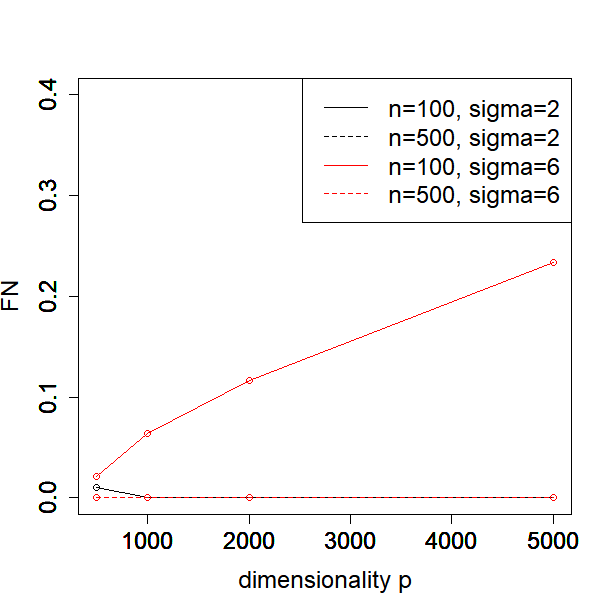 Figure 1
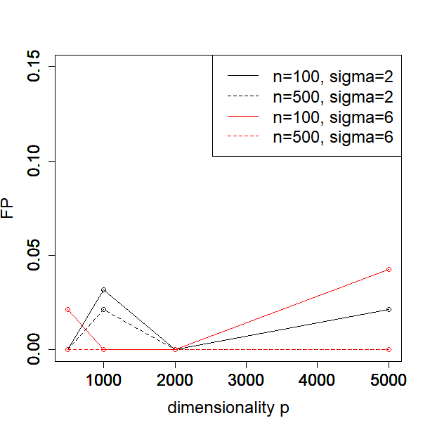 Figure 2
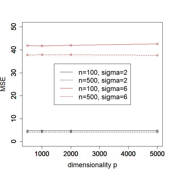 Figure 3
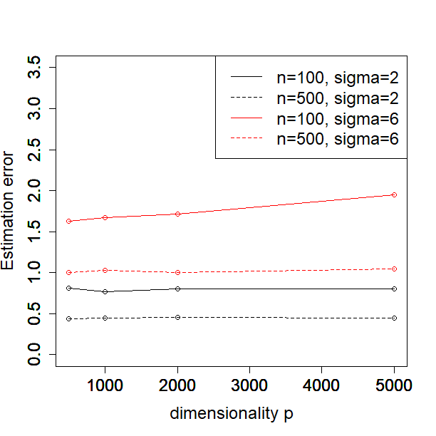 Figure 4
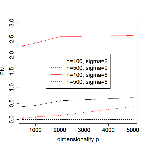 Figure 5
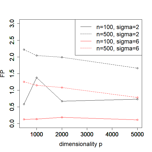 Figure 6
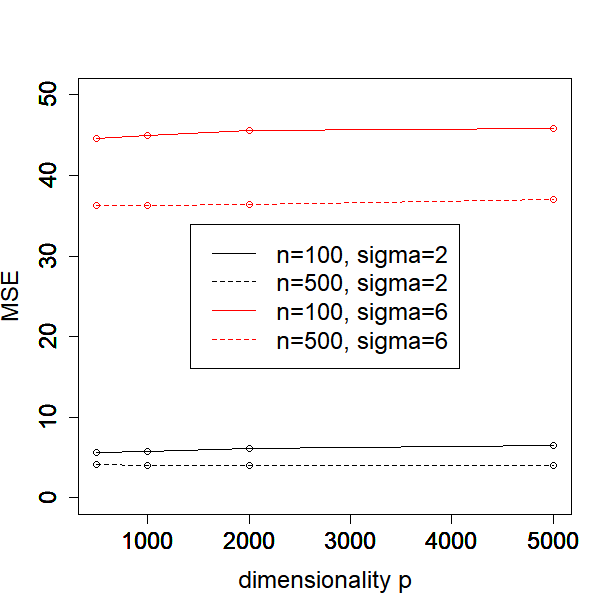 Figure 7
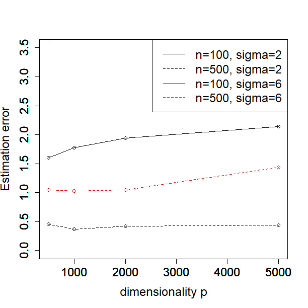 Figure 8
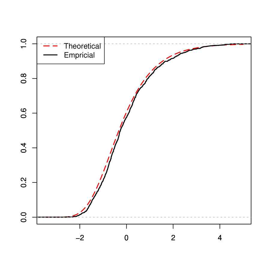 Figure 9
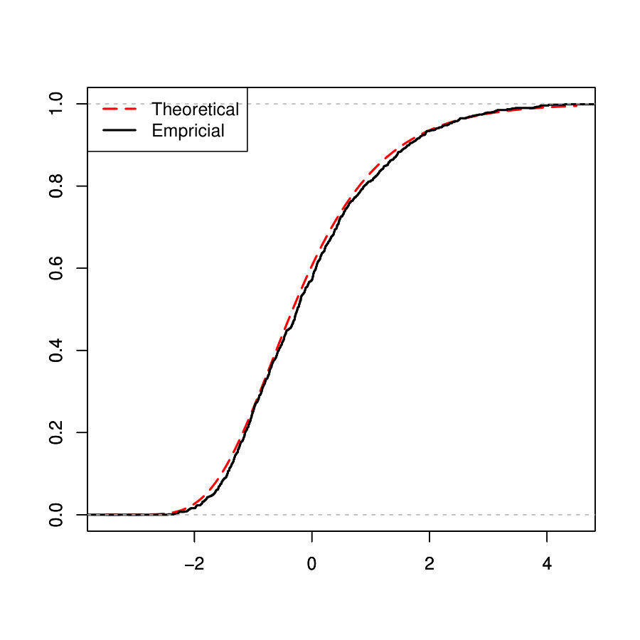 Figure 10
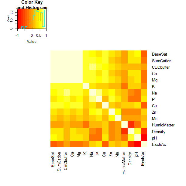 Figure 11
| Method | MSE | FN | FP | |
| Elnet | 5.94 (0.07) | 1.40 (0.03) | 0.00 (0.00) | 1.64 (0.24) |
| SIS-Elnet | 5.47 (0.06) | 1.30 (0.03) | 0.00 (0.00) | 1.15 (0.12) |
| LASSO | 5.95 (0.07) | 1.50 (0.03) | 0.00 (0.00) | 1.28 (0.18) |
| SIS-LASSO | 5.47 (0.06) | 1.42 (0.03) | 0.00 (0.00) | 0.85 (0.10) |
| SIS-Ridge | 86.00 (0.76) | 4.50 (0.01) | 0.00 (0.00) | 12.00 (0.00) |
| SIS-PACS | 4.69 (0.07) | 0.48 (0.02) | 0.00 (0.00) | 0.01 (0.01) |
| PCS | 4.74 (0.05) | 0.76 (0.02) | 0.00 (0.00) | 0.03 (0.02) |
| PRCS | 4.91 (0.05) | 0.93 (0.02) | 0.00 (0.00) | 2.55 (0.15) |
| Elnet | 6.42 (0.09) | 1.57 (0.03) | 0.00 (0.00) | 2.45 (0.26) |
| SIS-Elnet | 5.64 (0.06) | 1.41 (0.03) | 0.00 (0.00) | 1.28 (0.12) |
| LASSO | 6.41 (0.08) | 1.64 (0.04) | 0.00 (0.00) | 2.06 (0.21) |
| SIS-LASSO | 5.65 (0.06) | 1.52 (0.03) | 0.00 (0.00) | 1.03 (0.10) |
| SIS-Ridge | 88.74 (0.75) | 4.59 (0.01) | 0.00 (0.00) | 12.00 (0.00) |
| SIS-PACS | 4.97 (0.08) | 0.72 (0.02) | 0.00 (0.00) | 1.78 (0.43) |
| PCS | 4.77 (0.05) | 0.81 (0.03) | 0.00 (0.00) | 0.02 (0.02) |
| PRCS | 4.85 (0.06) | 0.89 (0.03) | 0.00 (0.00) | 1.21 (0.11) |
| Method | MSE | FN | FP | |
| Enet | 6.75 (0.08) | 2.45 (0.02) | 1.00 (0.01) | 0.98 (0.25) |
| SIS-Enet | 6.47 (0.10) | 2.30 (0.03) | 0.76 (0.05) | 3.16 (0.41) |
| LASSO | 6.75 (0.08) | 2.45 (0.02) | 1.00 (0.01) | 0.98 (0.25) |
| SIS-LASSO | 6.47 (0.10) | 2.30 (0.03) | 0.76 (0.05) | 3.16 (0.41) |
| SIS-Ridge | 14.14 (0.10) | 3.85 (0.00) | 0.27 (0.04) | 19.27 (0.04) |
| SIS-PACS | 6.53 (0.14) | 2.43 (0.04) | 1.06 (0.05) | 3.39 (0.73) |
| PCS | 5.24 (0.12) | 1.41 (0.08) | 0.34 (0.05) | 1.63 (0.13) |
| PRCS | 5.72 (0.13) | 1.75 (0.08) | 0.43 (0.05) | 1.34 (0.24) |
| Elnet | 7.16 (0.08) | 2.55 (0.02) | 1.02 (0.01) | 0.40 (0.09) |
| SIS-Elnet | 7.02 (0.09) | 2.49 (0.03) | 0.94 (0.03) | 1.31 (0.34) |
| LASSO | 7.16 (0.08) | 2.55 (0.02) | 1.02 (0.01) | 0.36 (0.08) |
| SIS-LASSO | 7.03 (0.09) | 2.49 (0.03) | 0.94 (0.03) | 1.31 (0.34) |
| SIS-Ridge | 14.40 (0.11) | 3.87 (0.00) | 0.59 (0.05) | 19.59 (0.05) |
| SIS-PACS | 7.28 (0.16) | 2.83 (0.04) | 1.26 (0.07) | 2.41 (0.95) |
| PCS | 5.96 (0.14) | 1.83 (0.09) | 0.63 (0.06) | 0.74 (0.08) |
| PRCS | 6.48 (0.13) | 2.14 (0.07) | 0.68 (0.05) | 0.73 (0.24) |
| Method | MSE | FN | FP | |
|---|---|---|---|---|
| Enet | 69.71 (0.88) | 5.13 (0.03) | 4.99 (0.13) | 1.57 (0.37) |
| SIS-Enet | 72.54 (0.88) | 5.25 (0.03) | 5.65 (0.10) | 0.23 (0.12) |
| LASSO | 72.78 (0.87) | 5.41 (0.03) | 6.06 (0.10) | 0.09 (0.04) |
| SIS-LASSO | 70.12 (0.86) | 5.35 (0.04) | 5.69 (0.12) | 0.94 (0.19) |
| SIS-Ridge | 109.66 (0.87) | 5.74 (0.01) | 4.46 (0.06) | 16.46 (0.06) |
| SIS-PACS | 71.27 (0.89) | 5.58 (0.02) | 5.06 (0.02) | 3.45 (0.07) |
| PCS | 58.87 (0.50) | 4.80 (0.04) | 4.95 (0.03) | 0.06 (0.06) |
| PRCS | 59.76 (0.56) | 4.83 (0.04) | 4.97 (0.02) | 0.00 (0.00) |
| Method | Classification Error | FN | FP | |
|---|---|---|---|---|
| Enet | 0.129 (0.003) | 5.79 (0.01) | 2.16 (0.17) | 12.77 (1.54) |
| SIS-Enet | 0.126 (0.003) | 5.69 (0.03) | 1.37 (0.15) | 7.48 (0.39) |
| LASSO | 0.136 (0.003) | 5.83 (0.01) | 4.19 (0.13) | 4.25 (0.49) |
| SIS-LASSO | 0.130 (0.003) | 5.75 (0.02) | 3.94 (0.12) | 3.50 (0.32) |
| SIS-Ridge | 0.311 (0.003) | 6.28 (0.01) | 0.11 (0.05) | 12.11 (0.05) |
| PCS | 0.098 (0.004) | 5.39 (0.05) | 1.73 (0.14) | 2.92 (0.31) |
| PRCS | 0.099 (0.004) | 5.34 (0.06) | 1.71 (0.13) | 3.26 (0.32) |
| Method | MSE | FN | FP | |
|---|---|---|---|---|
| Enet | 102.47 (1.84) | 3.90 (0.08) | 1.51 (0.12) | 4.88 (0.86) |
| SIS-Enet | 96.60 (2.74) | 3.49 (0.09) | 1.02 (0.12) | 4.20 (0.37) |
| LASSO | 103.11 (1.89) | 4.42 (0.08) | 2.30 (0.13) | 3.74 (0.71) |
| SIS-LASSO | 96.97 (2.78) | 4.27 (0.08) | 2.05 (0.14) | 1.87 (0.20) |
| SIS-Ridge | 226.52 (3.78) | 4.95 (0.03) | 0.26 (0.08) | 12.26 (0.08) |
| SIS-PACS | 89.82 (2.70) | 3.54 (0.15) | 0.26 (0.08) | 7.32 (0.45) |
| PCS | 79.79 (3.16) | 2.42 (0.14) | 0.42 (0.10) | 1.29 (0.33) |
| PRCS | 74.60 (1.24) | 2.15 (0.12) | 0.31 (0.08) | 0.06 (0.03) |
| Method | MSE | Model Size |
|---|---|---|
| Enet | 1.088 (0.047) | 3.70 (0.38) |
| LASSO | 1.068 (0.045) | 2.08 (0.21) |
| Ridge | 1.113 (0.044) | 15.00 (0.00) |
| PCS | 0.996 (0.062) | 5.82 (0.37) |
| PRCS | 1.028 (0.063) | 5.96 (0.38) |
| PCS | Enet | LASSO | |
|---|---|---|---|
| Variables | |||
| BaseSat | 16 | 9 | 0 |
| SumCaton | 32 | 23 | 0 |
| CECbuffer | 86 | 62 | 48 |
| Ca | 37 | 32 | 11 |
| Mg | 6 | 10 | 0 |
| K | 49 | 27 | 12 |
| Na | 22 | 10 | 6 |
| P | 32 | 15 | 5 |
| Cu | 47 | 17 | 9 |
| Zn | 29 | 17 | 4 |
| Mn | 69 | 43 | 32 |
| HumicMatt | 89 | 70 | 69 |
| Density | 25 | 15 | 4 |
| pH | 27 | 11 | 4 |
| ExchAc | 16 | 9 | 4 |
| Method | MSE | Model Size |
| SIS-Enet | 0.358 (0.015) | 15.66 (0.46) |
| SIS-Lasso | 0.356 (0.016) | 9.12 (0.18) |
| SIS-Ridge | 0.632 (0.024) | 26.00 (0.00) |
| PCS | 0.327 (0.014) | 15.04 (0.39) |
| PRCS | 0.361 (0.018) | 12.77 (0.37) |
Peer Reviews
No public reviews on file for this paper yet. If you reviewed it on a platform where reviews are public (OpenReview, ICLR, NeurIPS, ICML), you can paste yours below so the community can read it here.
Videos
No videos yet. Explain this paper in a talk, walkthrough, or lecture? Add one.
Taxonomy
TopicsStatistical Methods and Inference · Statistical Methods and Bayesian Inference · Advanced Statistical Methods and Models
Penalized linear regression with
high-dimensional pairwise screening
Siliang Gong, Kai Zhang and Yufeng Liu
University of Pennsylvania
and The University of North Carolina at Chapel Hill
Abstract: In variable selection, most existing screening methods focus on marginal effects and ignore dependence between covariates. To improve the performance of selection, we incorporate pairwise effects in covariates for screening and penalization. We achieve this by studying the asymptotic distribution of the maximal absolute pairwise sample correlation among independent covariates. The novelty of the theory is in that the convergence is with respect to the dimensionality , and is uniform with respect to the sample size . Moreover, we obtain an upper bound for the maximal pairwise R squared when regressing the response onto two different covariates. Based on these extreme value results, we propose a screening procedure to detect covariates pairs that are potentially correlated and associated with the response. We further combine the pairwise screening with Sure Independence Screening (Fan and Lv, 2008) and develop a new regularized variable selection procedure. Numerical studies show that our method is very competitive in terms of both prediction accuracy and variable selection accuracy.
Key words and phrases:Pairwise Screening, Penalized Regression, Sure Independence Screening, Variable Selection
1 Introduction
In the era of big data, high dimensional problems are of interest in many scientific fields, where the number of variables may be comparable to or even much larger than the sample size. For example, in genetic studies, one often has tens of thousands of genes in the microarray datasets with only a few hundreds of patients; in neuroscience, fMRI images may contain millions of voxels.
In recent years, much research effort has been devoted to dealing with high dimensional data analysis. Among those methods developed, penalized least squares plays an important role. In particular, one of the most well-known method is the LASSO proposed by Tibshirani (1996), which is the solution to the following penalized problem
[TABLE]
where is the penalty. Tibshirani (1996) showed that the LASSO leads to a sparse estimator that shrinks the OLS solution and sets some of the estimated coefficients to exact zero. Despite with good theoretical properties and practical performance, the LASSO has two major drawbacks: firstly, due to the shrinkage nature, LASSO may over-shrink the estimates and cause significant bias; secondly, if there is a group of variables that are highly correlated, LASSO tends to select only one of them. To address these issues, Zou and Hastie (2005) introduced the elastic net method, using as the regularization term in (1.1) and thus encouraging a grouping effect. Besides the elastic net, various penalized variable selection methods have been proposed as extensions to LASSO, including the Dantzig selector (Candès and Tao, 2007), the smoothly clipped absolute deviation (SCAD) penalty (Fan and Li, 2001), among many others. See Hastie et al. (2003) and Fan and Lv (2010) for a comprehensive overview.
For high dimensional variable selection, it is crucial to account for the dependency structure of covariates. Such structure information not only improves the accuracy of selection, but also have practical meanings. For instance, in gene expression data, genes usually function as biological pathways instead of working independently. Classical penalized variable selection methods, however, usually do not explicitly take into account the relationships between covariates. To address this problem, Yuan and Lin (2006) proposed the group LASSO method, which takes advantage of the grouping information among the covariates. Extensions of group lasso include, but are not limited to Breheny and Huang (2015). Other methods use the structure information as predictor graph (see Li and Li (2008); Pan et al. (2010); Zhu et al. (2013); Yu and Liu (2016) among others for reference).
A common assumption for the methods mentioned above is that the underlying predictor graph is given, which may not hold in practice. When the prior information is not available, the idea of clustering can be incorporated to improve regression performance. Specifically, Park et al. (2007) proposed to perform hierarchical clustering on the covariates first and take the cluster average as new predictors for regression. There are also methods using supervised clustering to encourage highly correlated pairs of covariates to be included or excluded simultaneously (Bondell and Reich, 2008; Sharma et al., 2013). Similarly, another type of methods aims to make correlated covariates have similar regression coefficients (She, 2010). Nevertheless, a large sample correlation between two variables does not necessarily indicate that they are dependent in the population sense. When the dimensionality continues to increase, the maximal pairwise correlation among independent covariates can be close to 1 (Fan and Lv, 2010). Therefore, it is important to identify covariates that are truly correlated and incorporate such information into variable selection procedures.
In this paper, we study the limiting behavior of the maximal absolute pairwise sample correlation among covariates when they are independent Gaussian random variables. Different from existing work, we investigate the limiting distribution as the dimensionality diverges. Therefore, the proposed asymptotic results potentially can be applied to datasets with arbitrarily large dimensionality. We further discuss the extreme behavior of the maximal absolute Spearman’s rho statistic for covariates with general distributions. On the other hand, we obtain the upper bound of maximal pairwise R squared when regressing the response onto pairs of covariates. With the extreme value results, we formulate a screening procedure to identify covariates pairs that are potentially dependent and associated with the response. We further combine the pairwise screening with the Sure Independence Screening (SIS) (Fan and Lv, 2008) and propose a novel penalized variable selection method. More specifically, we assign different penalties to each individual covariate according to the screening results. Numerical experiments show that the performance of our proposed method is competitive compared with existing approaches in terms of both variable selection and prediction accuracy.
The remainder of this paper is organized as follows: We first investigate the limiting distribution of the maximal pairwise sample correlation among covariates in Section 2.1. We also show that our asymptotic results cover that of Cai and Jiang (2012) as a special case. Then we propose an upper bound for the maximal pairwise R squared in Section 2.2. In Section 3.1 we formulate our proposed variable selection approach as a penalized maximum likelihood problem, and discuss potential extensions of our method in Section 3.2. Theoretical properties are discussed in Section 4. We show with simulated experiments as well as two real datasets in Section 5 that the proposed method has improved performance when important variables are highly correlated. Finally, we conclude this paper and discuss possible future work in Section 6. Proofs of the theoretical results are provided in the Appendix.
2 Pair Screening for covariates
Suppose we have the following linear model
[TABLE]
where is the response vector, is an design matrix with being independent and identical observations from the covariate . We assume that the covariate vector has a multivariate distribution with unknown covariance matrix , and is a vector of i.i.d. random variables with mean 0 and standard deviation , and is independent of the covariate vector .
For the linear model (2.2), variable selection methods aim to identify the non-zero components of , in other words, the important variables among all candidate predictors. Particularly, if two covariates have a large pairwise correlation, we may want to include or exclude these two variables simultaneously when conducting variable selection. However, the sample correlation can be spurious, especially when the number of covariates is relatively large. Therefore, it is important to identify covariates that are truly correlated. In other words, we need to find a threshold for the pairwise sample correlation among covariates to screen covariates pairs. In the following subsection, we will discuss in details the asymptotic results that generate the screening rule.
2.1 Extreme laws of pairwise sample correlation among covariates
We propose to choose a bound based on the extreme laws of the pairwise sample correlation when the covariates are independent. Our investigations are under two settings: (a) the covariates are normally distributed; (b) the covariates are non-Gaussian random variables.
2.1.1 Gaussian covariates
It has been recently studied that the maximal absolute Pearson sample correlation between i.i.d. Gaussian covariates and an independent response has a Gumble-type limiting distribution as goes to infinity (Zhang, 2017). Motivated by Zhang (2017)’s work, we find that the maximal absolute pairwise sample correlation among independent covariates also has a limiting distribution, as stated in the following theorem:
Theorem 1**.**
Suppose are independent Gaussian variables and we observe independent samples from each of ’s. Let , where is the Pearson sample correlation between and . Then as ,
[TABLE]
which is uniformly for any . Here , , and c_{p,n}=\big{(}\frac{n-2}{2}B(\frac{1}{2},\frac{n-2}{2})\sqrt{1-p^{-4/(n-2)}}\big{)}^{2/(n-2)} are the normalizing constants.
In random matrix theory, is also known as the coherence when the design matrix is random. Specifically, the coherence is defined as the largest magnitude of the off-diagonal entries of the sample correlation matrix associated with a random matrix. The limiting behavior of the coherence has been well studied when the sample size goes to infinity. For example, Cai et al. (2011) studied the asymptotic distribution under certain regularity conditions with application to the testing of covariance matrix. Cai and Jiang (2012) further obtained the limiting laws of the coherence for different divergence rate of with respect to and summarized the results as phase transition phenomena. We can show that our result unifies the convergence in terms of the sample size, and covers Cai and Jiang (2012)’s as special cases, described in the following corollary.
Corollary 1**.**
Let be defined as in Theorem 1, where we still assume ’s are independent normal random variables. Let .
- (a)
(Sub-Exponential Case) Suppose as and , then as ,
[TABLE] 2. (b)
(Exponential Case) Suppose satisfies as . Then as ,
[TABLE]
where K(\beta)=\big{(}\frac{\beta}{2\pi(1-4e^{-4\beta})}\big{)}^{1/2}. 3. (c)
(Super-Exponential Case) Suppose satisfies as . Then as ,
[TABLE]
Compared with previous work, our asymptotic distribution is novel in two aspects. First, the convergence in Theorem 1 is with respect to instead of , making it applicable to high dimensional data, or even ultrahigh dimensional problems. Moreover, the convergence result we have discovered is uniform for any , thus finite sample performance is guaranteed.
2.1.2 Non-Gaussian covariates
When the covariates are non-Gaussian random variables, it is more desirable to choose a distribution-free statistic for the screening rule. Therefore, instead of using the Pearson’s sample correlation, we study the extreme behavior of the Spearman’s rho statistic (Spearman, 1904). Recall that are i.i.d. observations from the covariate . Let and be the ranks of and in and respectively. Then the Spearman’s rho is defined as
[TABLE]
where .
Similar to the normal setting, we are particularly interested in the limiting distribution of when the covariates are all independent, which has been studied in Han and Liu (2014). The following proposition states that as increases, converges to a Gumble type distribution.
Proposition 1**.**
Suppose that are independent and identically distributed random variables, and we have independent samples for each of the covariates. Let be the squares of the maximal pairwise Spearman’s rho statistics, then for , we have
[TABLE]
Theorem 1 and Proposition 1 characterize the magnitude of the maximal pairwise correlation and Spearman’s rho statistic respectively when the covariates are independent. Suppose a pair of covariates, say and , have a absolute sample correlation greater than the quantile of the distribution given in Theorem 1 or Proposition 1, then they tend to be marginally dependent. Since we are only interested in pairs of truly important covariates, we further investigate the extreme behavior of the maximal pairwise R squared under the null model, i.e., ’s are all equal to zero.
2.2 R squared screening for pairs of covariates
With the asymptotic distributions introduced in the previous subsections, we can identify covariates pairs that are potentially dependent. However, such screening does not take into account the association between the covariates and the response. It is possible that an important variable has a large sample correlation with unimportant ones; or two highly correlated covariates are both unrelated to the response. To address such an issue, we introduce another screening procedure based on the R squared from regressing the response onto the pairs of covariates.
Consider the linear regression where we regress onto a pair of covariates and with , we can obtain the corresponding R squared . Under the model setting (2.2), when all the coefficients are zeros, the maximal pairwise R squared cannot be too large. In fact, there exists an asymptotic bound for , as described in the following theorem.
Theorem 2**.**
Let , where is the pairwise squares from regressing onto and where . Suppose that and are from the model setting 2.2 and we further assume that is a normally distributed. Then when ’s are all zeros, we have for any fixed , , as , .
With the bound given by Theorem 2, we can design a screening rule to find pairs of covariates that are potentially associated with the response. In Section 3, we introduce how to make use of the theoretical results to benefit variable selection.
3 Penalized variable selection using pairwise screening
In this section, we propose a pairwise screening procedure that takes advantages of the asymptotic results in Section 2. We further establish a new penalization algorithm for variable selection.
3.1 Screening-based penalization
Given the limiting distribution of the maximal pairwise sample correlation described in Section 2, we propose the following screening rule to identify covariates pairs that are potentially correlated and related to the response:
[TABLE]
where is the quantile of the distribution given in Theorem 1 (for Gaussian covariates) or Proposition 1 (for non-Gaussian covariates), and . Note that the values of and can affect the size of . The larger and are, there are fewer pairs included in . In practice, we suggest to take and .
The group definition in (3.6) is a screening procedure with respect to covariates pairs. The idea of screening is prevalent for high dimensional data analysis. In particular, for penalized variable selection methods, increasing dimensionality makes it more difficult to capture the inherent sparsity structure. Therefore, dimension reduction is necessary when there are tens of thousands of candidate variables. To this end, Fan and Lv (2008) introduced the Sure Independence Screening (SIS) method, which ranks the covariates based on the magnitude of their sample correlation with the response. More specifically, let be a vector such that and is a constant between , then a sub-model is defined as
[TABLE]
where denotes the integer part of . Fan and Lv (2008) further demonstrated that SIS is screening consistent under some conditions. This guarantees that all those ’s with are included in the subset of covariates.
To take advantage of the distribution information while implementing dimension reduction, we propose a new penalized variable selection approach that applies different penalties to each covariate based on the screening results. Let be the index set of covariates that have the largest absolute sample correlation with the response among . We also define the set of paired covariates as
[TABLE]
Our proposed method is established by solving the following optimization problem:
[TABLE]
subject to for . In other words, we ignore the covariates that fail the marginal screening.
From the above penalty, it can be seen that we apply different penalties to covariates based upon the results from two types of screening. The intuitions behind the proposed penalty are
- •
For a covariate that is included in both and , we only apply the penalty because it tends to be an important variable that we need to include in the final model.
- •
For a covariate that is included in but not in , we only apply the penalty since there is no significant multicollinearity between it and other covariates.
- •
For a covariate that is not included in , since it does not pass the marginal screening, we no longer consider it in the regression. This is because SIS enjoys screening consistency under certain assumptions, which implies that covers all important variables.
Our proposed method is connected with existing penalization approaches when the covariates have certain covariance structure. In particular, when the covariates are all independent, our method reduces to SIS-LASSO, which performs marginal screening first and then implements LASSO on the remaining covariates; when the predictors are all highly correlated such that includes all covariates pairs, our method is equivalent to SIS-Ridge.
So far we have established a new penalized variable selection. Now we discuss how to solve the optimization problem in (3.9). One can see that the penalty part of (3.9) is convex, so we can efficiently solve it by coordinate descent algorithm (Friedman et al., 2010). Specifically, the updating rule has the following form:
[TABLE]
where is the fitted value excluding the effect of , and is the soft-thresholding function. In practice, we can first implement SIS to obtain when the dimension is high, then run the algorithm on the covariates ’s with .
Remark 1**.**
The computational cost of the pairwise screening procedure is , which can be very inefficient as increases. In our proposed procedure, to reduce the computational complexity, we implement the marginal screening first to obtain . Since the cardinality of is , the computational cost of applying pairwise screening to will reduce to O\big{(}(n/\log(n))^{2}\big{)}.
3.2 Further extensions
As discussed in the previous subsection, we introduce a new penalized method that combines marginal screening with pairwise screening under the linear model setting. Note that the pairwise covariates screening does not involve the response. Therefore, our method can be further extended to generalized linear models (GLM), e.g., logistic regression for binary response, or cox model for survival data. Suppose the response is from the following one-parameter exponential family . Moreover, we assume for generalized linear models.
Similar to 3.6, we define the pairwise screening as
[TABLE]
The difference is that we do not consider the R squared screening for GLMs. This is because for GLMs, it is not reasonable to use the regression R squared to evaluate the associations between the covariates and the response. We further define the set of paired covariates as follows
[TABLE]
Let be our proposed screening-based penalty. Then for logistic regression, we need to solve the following penalized maximum likelihood problem
[TABLE]
In the above optimization problem, the log likelihood part can be approximated by a quadratic function, which is a weighted least squares term (Friedman et al., 2010). Therefore, it can still be solved by coordinate descent algorithm. Similarly, we can use the algorithm proposed by Simon et al. (2011) to solve the regularized Cox proportional hazard model using the screening based penalty .
4 Theoretical properties
In this section, we study the theoretical properties of the proposed pairwise correlation screening (PCS) method. More specifically, we investigate the conditions under which the PCS achieves the variable selection consistency.
Note that we implemented the marginal screening using SIS to the covariates set. Fan and Lv Fan and Lv (2008) demonstrated that under certain regularity conditions, SIS has the screening consistency, that is, the resulting subset of covariates includes all important variables. Due to space constraints, we only present the main result. The regularity conditions are provided in the appendix.
Proposition 2** (Fan and Lv (2008)).**
Under , if , then there is some such that , when with , we have, for some ,
[TABLE]
where is the subset of covariates obtained from the sure independence screening.
The above proposition guarantees that all important variables survive the marginal screening with high probability. In order to achieve the selection consistency, we also need to ensure that only important variables can pass the pairwise screening. In the following theorem, we present the technical conditions that are required such that the event occurs with high probability.
Theorem 3**.**
Suppose the following conditions holds
- ()
. 2. ()
There exists such that either one of the following two conditions holds:
- (a)
** 2. (b)
.
Here denotes the population correlation between covariates and . Then under conditions and or conditions and , we have that as ,
[TABLE]
Given Proposition 2 and Theorem 3, to demonstrate the selection consistency of PCS, we only need to show that the penalty in (3.9) can identify the important variables in exactly. This relates to the selection consistency for the LASSO, which has been studied extensively. In particular, Zhao and Yu Zhao and Yu (2006) have shown that the Irrepresentable Condition (to be clarified later) is almost necessary and sufficient for LASSO to select all important variables.
We first introduce some necessary notations. Let . Without of loss of generality, assume that where for and otherwise. By Theorem 3, we further assume that where . Then the design matrix can be expressed as , where corresponds to the first columns, corresponds to the th to the th columns and corresponds to the last columns of respectively. Similarly, we can write , , and .
Set , , , , , , , , . Then can be expressed in a block-wise form as follows:
[TABLE]
We impose the following assumption analogous to the Irrepresentable Condition introduced by Zhao and Yu Zhao and Yu (2006). Specifically, we assume that there exists a constant , such that
[TABLE]
where is the max norm.
In fact, we can show that the condition mentioned above is implied by the Irrepresentable Condition on the full covariates set under mild assumptions. We illustrate this result in the following theorem:
Theorem 4**.**
Assume that there exists so that , , and conditions and holds. Suppose the Irrepresentable Condition holds, i.e., s.t.
[TABLE]
where , , and is a positive constant. Then with probability tending to 1, the condition (4.16) holds.
The assumptions , in Theorem 4 require that and have eigenvalues bounded below. Given the Irrepresentable Condition in (4.17), we need additional constraints on the random noise ’s and the coefficients of important variables .
- ()
’s are i.i.d. random variables with finite ’s moment for an integer . 2. ()
There exists and such that .
So far we have discussed all the theoretical assumptions required to ensure the selection consistency of the proposed PCS method. We conclude the consistency result in the following theorem:
Theorem 5**.**
Suppose conditions (A1)–(A4), (C1)–(C2) and inequality (4.17) hold, and the assumptions of Theorem 4 are satisfied, then for any such that and , we have,
[TABLE]
where is the solution to (3.9).
The proof follows immediately from Proposition 2 and Theorems 3 and 4 as well as the selection consistency of the LASSO. It shows that under certain conditions, our proposed method is consistent in variable selection. In Section 5, we will show with numerical examples that our proposed method can perform well in practice.
5 Numerical Studies
In Section 3, we have established a new regularized variable selection approach for high-dimensional linear models. In this section, we demonstrate the performance of our proposed method using both simulations and real data examples.
5.1 Simulation study
In this section, we use several simulated examples to show that our method with pairwise correlation screening (PCS) or pairwise rank-based correlation screening (PRCS) outperforms some existing variable selection procedures. More specifically, PCS denotes our proposed method using the limiting distribution in Theorem 1, and PRCS uses the asymptotic result in Proposition 1.
For comparison, we consider LASSO, elastic net (Enet), SIS-LASSO, SIS-elastic net (SIS-Enet) and SIS-PACS. The SIS-PACS refers to applying the PACS method proposed by Sharma et al. (2013) after implementing the SIS procedure. In SIS-type methods, we first implement SIS and find those covariates with the largest absolute sample correlations with the response, then perform LASSO, Enet or PACS on these variables. We evaluate the variable selection accuracy using False Negatives (FN) and False Positives (FP). FN is defined as where denotes the indicator function, and FP is defined as We use the following quantities to evaluate the prediction accuracy:
- •
: the distance between the estimated coefficient vector and the true coefficients ;
- •
Out of sample mean squared errors (MSE) on the independent test data;
We generate the simulated data from Model (2.2) and conduct 100 replications. Each simulated dataset includes a training set of size 100, an independent validation set of size 100 and an independent test set of size 400. Here we fix the sample size to be 100 throughout the simulation study. In the next subsection, we also consider varying sample size for sensitivity study. We only fit models on the training data, and we use the validation data to select tuning parameters. Given the fitted model, we can calculate the FN, FP and the estimation error , and we make predictions and calculate the out of sample MSEs using the test data. We simulate the covariates from the multivariate Gaussian distribution , with being the correlation matrix.
Details of the simulated examples are as follows:
Example 1: We consider or , , and we take where the first 10 coefficients being non-zero and equal to 2. We set for , and [math] for all the other . We also consider and present the results in the supplementary. In other words, there are two groups in the covariates, where each group has 5 important variables.
Example 2: We consider or , , , where the first 3 coefficients are non-zero ones. We also consider and present the results in the supplementary. We generated Gaussian covariates with for .
Example 3: The coefficients have the same set up as in Example 1. But we set for and [math] for all the other . Therefore only part of the important variables are highly correlated. We consider and in this Example.
Example 4: In this example, we examine the performance of all methods under the logistic regression setting. We simulate the binary response from the binomial distribution , where , and follow the same set ups as in Example 1. We consider and in this Example. Instead of comparing MSE, we calculate the classification errors on the test data. We did not compare with SIS-PACS in this example since the R program does not support GLM.
Example 5: In this example, we generate the covariates from a multivariate distribution, where ’s are distributed with degrees of freedom 5. The covariance structure of the covariates and the coefficients are set the same as in Example 1. We consider and in this Example.
The results for simulated Example 1 is shown in Table 1. We see that when there are groups in the covariates, the performance improvement of our approach is significant compared with other penalized methods. While elastic net-based procedures perform better than LASSO-type approaches in terms of FN, as illustrated by Zou and Hastie (2005), they still miss approximately one important covariate on average. In contrast, the model selection results of our method are much closer to the correct model for this example. In addition, although SIS-PACS has competitive performance when is small, it tends to include more unimportant variables into the model when the noise level increases, and therefore may not work well.
Table 2 displays the performance comparisons for Example 2. Compared with Example 1, this setting is a more difficult one for our method, since correlation exists among all pairs of covariates. Nevertheless, PCS and PRCS perform better than, or as well as all the others in terms of estimation error and prediction accuracy. Moreover, besides SIS-Ridge, our proposed methods are able to identify more important variables than others in this example when the noise level is low.
Table 3 shows the results for Example 3, where correlation exists only within part of the important variables. This example is more difficult compared with Example 1 due to the correlation structure of the covariates. One can see that the false negatives are significantly larger for all procedures. Nevertheless our method still outperforms all the others in terms of prediction and variable selection accuracy.
Example 4 considers the logistic regression setting, and the results are provided in Table 4. One can see that as the correlations among the covariates vary, the performance of our method is always competitive compared with the others.
Table 5 displays the results for all methods under the non-Gaussian covariates setting. Similar to Example 1, our proposed PCS and PRCS achieve much better performance compared with the competitors. Moreover, due to the non-Gaussian set ups, the nonparametric method PRCS outperforms PCS.
As a conclusion, our method can make use of the correlation structure among predictors. Compared with other penalized variable selection procedures, our method performs well, especially when the covariates are highly correlated.
5.2 Sensitivity Study
In this subsection, we investigate how the performance of our method depends on the sample size, dimensionality, and noise level. In particular, we consider or , or and or in the Simulated Example 1 as introduced in Section 5.1. We illustrate the MSE, , FN and FP against different values of for each configuration of sample size and noise level in Figure 1.
One can see from the plots that the performance of PCS does not change much as the dimensionality increases from 500 to 5000, especially in terms of MSE and the estimation error of . Moreover, the performance is better when the sample size and signal to noise ratio (SNR) become larger, which is expected. In general, our proposed PCS method is robust to sample size, dimensionality and SNR.
5.3 Soil data
We first demonstrate the performance of our method in real applications using a small dataset. This dataset contains 15 covariates of soil characteristics for 20 plots with the same area in the Appalachian Mountain. The outcome variable is the forest diversity for each plot. More descriptions of the data can be found in Bondell and Reich (2008). To better demonstrate the correlation structure of covariates, we obtain the absolute pairwise correlation matrix and show the heatmap in Figure 2. One can see that some predictors are highly correlated. In particular, the magnitude of the pairwise correlations among Sum of Cations (SumCation), calcium, magnesium, Base Saturation (BaseSat), and cation exchange capacity (CEC) are as large as 0.9. The reason is SumCation, BaseSat, CEC are characteristics for cations; while calcium and magnesium are examples of cations (Bondell and Reich, 2008).
We conduct a total of 100 replications. In each replication, 15 samples are randomly chosen as the training set and the remaining as the test set. As in the simulation experiments, we applied LASSO, Enet, Ridge and our proposed PCS, PRCS to the dataset. For each method, 5-fold cross-validation is used to choose the tuning parameters since the sample size is very small. We report the average prediction errors on the test data and the model size in Table 6. One can see that PCS and PRCS outperform all the others in terms of prediction accuracy. Moreover, PCS and PRCS tend to include more covariates into the model compared with LASSO and Enet.
To further investigate the performance of variable selection, we summarize the frequency that each covariate is selected for LASSO, Enet and our method, which is displayed in Table 7. Note that among those variables that are most frequently selected by LASSO and Enet, for instance, CEC, Mn, HumicMatt, they also tend to be included for our method. Moreover, our method can identify covariates that are strongly correlated. For example, potassium, sodium and copper are variables related to cations, and all have a large sample correlation with CEC, which is a potentially important variable. These variables are frequently selected by our method, but not by Enet and LASSO.
5.4 Riboflavin data
In this section, we consider a real data set about the riboflavin production in Bacillus subtilis. The data contain samples, where the response variable is the logarithm of the riboflavin production rate, and the covariates are the logarithm of expression levels of genes. More descriptions about the dataset can be found in Bühlmann et al. (2014). Before analysis, all covariates are standardized to have zero means and unit standard deviations.
For comparison purpose, we apply LASSO, Enet, SIS-LASSO, SIS-Enet, SIS-ridge and our method to the dataset. We conduct 100 replications, and we randomly split the dataset into a training set of size with the remaining as the test data. For all methods, we implement 10-fold cross validation on the training data to select the penalty parameters.
The results are reported in Table 8. One can see that PCS has significant improvement in terms of out of sample mean squared errors compared with other competitors. On the other hand, PRCS does not perform well compared with PCS. A possible reason is that in this dataset all the variables have been taken log transformations and are approximated well by Gaussian distribution. Moreover, due to the assumption of Proposition 1 where , PRCS is more sensitive to the dimensionality and the sample size of dataset. As a result, PRCS may not achieve good performance when the dimensionality is too high.
We also examine the gene selection results. There are 8 genes that are selected at least 50 times out of the 100 replications by our method, i.e., XTRA_at, YCKE_at, YDAR_at, YOAB_at, YWFO_at, YXLC_at, YXLD_at and YXLE_at. Besides YXLC_at, all the other genes also appear among the most frequently selected genes by SIS-Enet and SIS-LASSO with a frequency no less than 50. For YXLC_at, we find that the magnitude of the pairwise sample correlations between this gene and two other genes, YXLD_at and YXLE_at, are greater than 0.95. It indicates that our method is capable of identifying potentially important variables that are highly correlated with the others.
6 Discussion
In summary, we propose a novel variable selection method that regularizes covariates selectively based on the results from two screening procedures: pairwise screening and marginal screening. The screening process of covariates pairs takes advantage of the distribution information of the maximal absolute pairwise sample correlation among covariates, and is applicable to large scale problems. Simulation experiments and real data study demonstrate that the proposed method performs well when important variables are highly correlated compared with existing approaches. For future research, we can consider other extensions of our proposed method, for example, the Cox model for survival data.
Appendix A Technical Proofs
We present some regularity conditions and key proofs in the appendix.
Regularity Conditions for Sure Independence Screening Define , . Let be the index set of covariates with non-zero coefficient. The following assumptions are imposed:
- ()
and for some , where is given by condition (A3). 2. ()
has a spherically symmetric distribution, and such that
[TABLE]
holds for any submatrix of with . 3. ()
, and for some and ,
[TABLE] 4. ()
There are some and such that .
Proof of Theorem 1.
To prove Theorem 1, we need to use the following lemma, which is from Arratia et al. (1989).
Lemma 1**.**
Let be an index set and be a set of subsets of , that is, for each . Let also be random variables. For a given , set . Then
[TABLE]
where , and , and is the -algebra generated by . In particular, if is independent of for each , then =0.
In our proof, we take Let we define one of and or , but , and , where . Let , by the Chen-Stein method (in particular, Lemma 6.2 in Cai and Jiang (2011)),
[TABLE]
where , and , .
Moreover, we have .
Since are independent, and are also independent with equal probability. Therefore we have .
On the other hand, . Take , where , and c_{p,n}=\big{(}\frac{n-2}{2}B(\frac{1}{2},\frac{n-2}{2})\sqrt{1-p^{-4/(n-2)}}\big{)}^{2/(n-2)}. Then
[TABLE]
Therefore, uniformly for any , , and \lim_{p\rightarrow\infty}\lambda_{p,n}=\frac{1}{2}\big{(}1-\frac{2}{n-2}x\big{)}^{\frac{n-2}{2}}
Then it follows from (A.19) that uniformly for any and ,
[TABLE]
When , . Therefore, uniformly for any ,
[TABLE]
Combining (A.21) and (A.22) we have uniformly for any ,
[TABLE]
Or equivalently,
[TABLE]
∎
Proof of Theorem 3.
Let event , event where , is the screening threshold for pairwise correlation screening. Then implies that no pairs of unimportant variables passed the R squares screening. implies that important and unimportant variables can not be too highly correlated.
By the definition of , we have
[TABLE]
For the event , we have
[TABLE]
Under the assumption , as . Therefore we have .
Next we show that as . We have
[TABLE]
where is the quantile of the limiting cumulative distribution function of the maximal pairwise correlation statistic, and we denote by .
Note that
[TABLE]
Let be the population correlation coefficient between and . Write , . It has been shown that as ,
We have
[TABLE]
where .
If as , then . Therefore , which yields . Then the tail probability in (A.26) goes to zero as . It follows that as .
If as , then . Under assumption that , . Again the tail probability in (A.26) goes to zero as . It follows that as .
If as , then . Hence . Under the assumption , we have . Therefore as .
Given and , we have as . ∎
Proof of Theorem 4.
It follows from (4.17) directly that
[TABLE]
where denotes the max norm of a matrix. Based the definition of , we have the following element wise inequalities , . Here is the pairwise correlation screening bound. Since is positive definite, there exists an orthogonal matrix s.t. , where is a diagonal matrix consists of the eigenvalues of . By assumption, we have . Therefore Under the assumption that , . It follows that . By assumption , . Thus , then = as . Therefore
[TABLE]
Write , and . Then the above term becomes . Moreover, we have
[TABLE]
Since , and
[TABLE]
Therefore we have
[TABLE]
as . It follows that with probability tending to 1 as which concludes the proof if we take . ∎
The reference list from the paper itself. Each links out to its DOI / PubMed record.
- 1Arratia et al. (1989) Richard Arratia, Larry Goldstein, and Louis Gordon. Two moments suffice for poisson approximations: the chen-stein method. The Annals of Probability , 17(1):9–25, 1989.
- 2Bondell and Reich (2008) Howard D Bondell and Brian J Reich. Simultaneous regression shrinkage, variable selection, and supervised clustering of predictors with oscar. Biometrics , 64(1):115–123, 2008.
- 3Breheny and Huang (2015) Patrick Breheny and Jian Huang. Group descent algorithms for nonconvex penalized linear and logistic regression models with grouped predictors. Statistics and Computing , 25(2):173–187, 2015.
- 4Bühlmann et al. (2014) Peter Bühlmann, Markus Kalisch, and Lukas Meier. High-dimensional statistics with a view toward applications in biology. Annual Review of Statistics and Its Application , 1:255–278, 2014.
- 5Cai and Jiang (2012) T Tony Cai and Tiefeng Jiang. Phase transition in limiting distributions of coherence of high-dimensional random matrices. Journal of Multivariate Analysis , 107:24–39, 2012.
- 6Cai et al. (2011) T Tony Cai, Tiefeng Jiang, et al. Limiting laws of coherence of random matrices with applications to testing covariance structure and construction of compressed sensing matrices. The Annals of Statistics , 39(3):1496–1525, 2011.
- 7Candès and Tao (2007) Emmanuel Candès and Terence Tao. The dantzig selector: Statistical estimation when p is much larger than n. The Annals of Statistics , 35(6):2313–2351, 2007.
- 8Fan and Li (2001) Jianqing Fan and Runze Li. Variable selection via nonconcave penalized likelihood and its oracle properties. Journal of the American Statistical Association , 96(456):1348–1360, 2001.