Maximum Likelihood Detection in a Four-Dimensional Stokes-Space Receiver
Amir Tasbihi, Frank R. Kschischang

TL;DR
This paper derives a maximum likelihood detection rule for a four-dimensional optical receiver, compares three detection algorithms, and evaluates their performance and achievable rates through simulations and approximations.
Contribution
It introduces simplified detection algorithms with negligible performance loss and provides high-SNR approximations and achievable rate analyses for four-dimensional optical signals.
Findings
Successive detection reduces complexity by a factor of 8 with minimal performance loss.
High-SNR approximation is accurate even at low SNRs.
Achievable rates of 10 bits per channel use at 25 dB SNR for specific constellations.
Abstract
The maximum likelihood detection rule for a four-dimensional direct-detection optical front-end is derived. The four dimensions are two intensities and two differential phases. Three different signal processing algorithms, composed of symbol-by-symbol, sequence and successive detection, are discussed. To remedy dealing with special functions in the detection rules, an approximation for high signal-to-noise ratios (SNRs) is provided. Simulation results show that, despite the simpler structure of the successive algorithm, the resulting performance loss, in comparison with the other two algorithms, is negligible. For example, for an 8-ring/8-ary phase constellation, the complexity of detection reduces by a factor of 8, while the performance, in terms of the symbol error rate, degrades by 0.5 dB. It is shown that the high-SNR approximation is very accurate, even at low SNRs. The achievable…
Click any figure to enlarge with its caption.
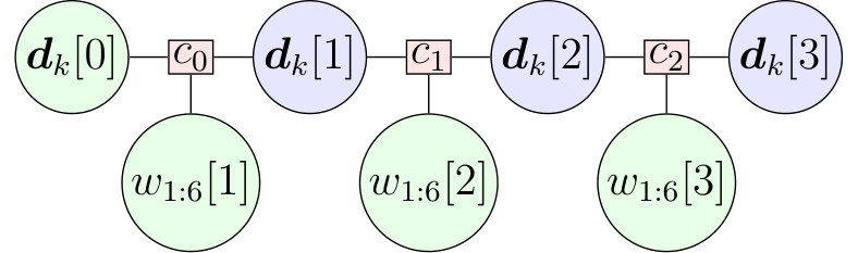 Figure 1
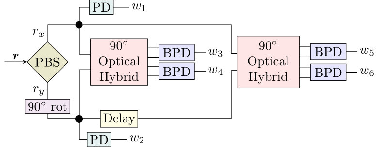 Figure 2
 Figure 3
 Figure 4
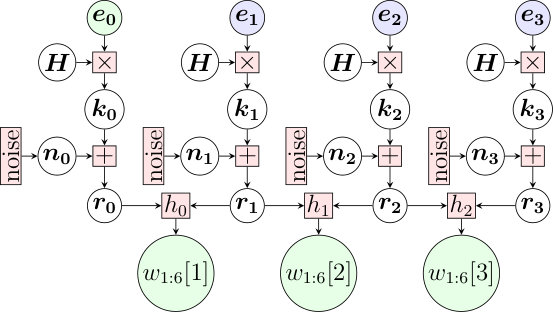 Figure 5
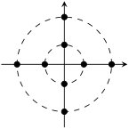 Figure 6
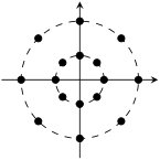 Figure 7
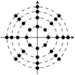 Figure 8
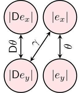 Figure 9
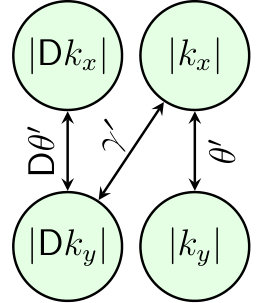 Figure 10
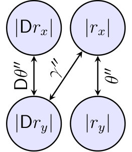 Figure 11
 Figure 12
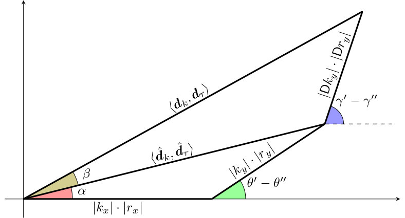 Figure 13
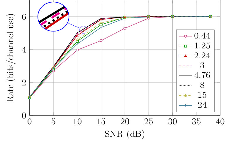 Figure 14
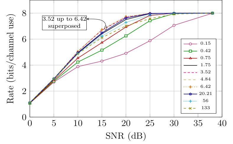 Figure 15
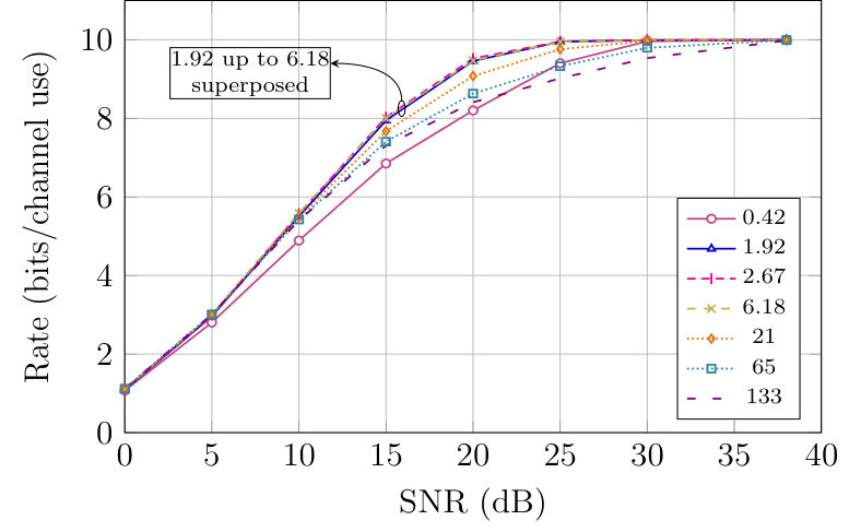 Figure 16
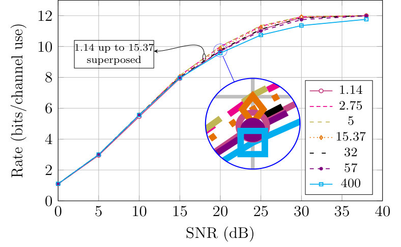 Figure 17
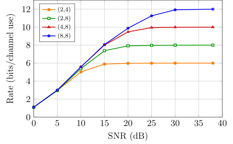 Figure 18
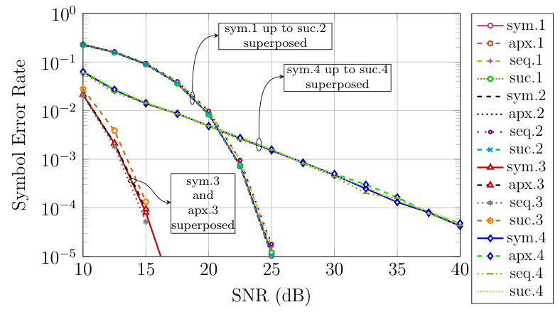 Figure 19
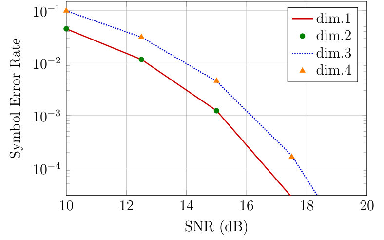 Figure 20
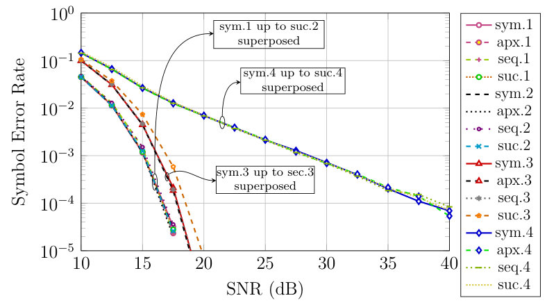 Figure 21
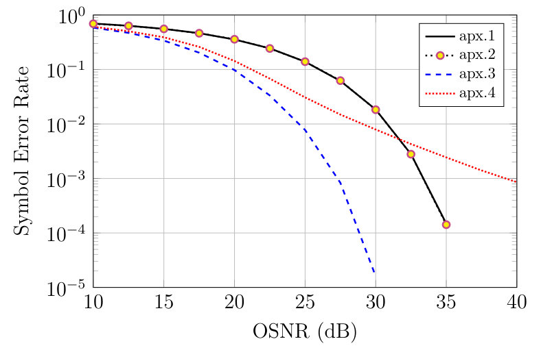 Figure 22
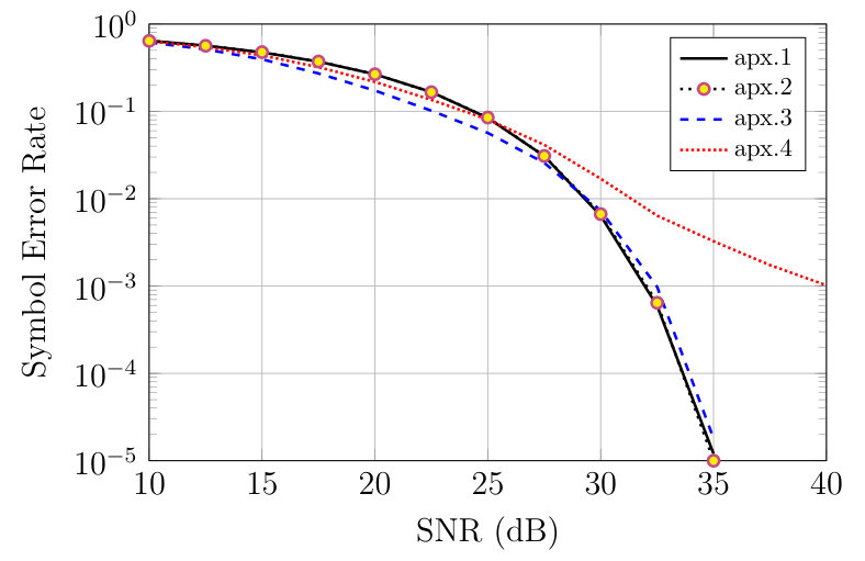 Figure 23
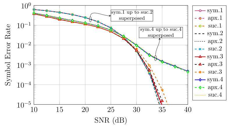 Figure 24
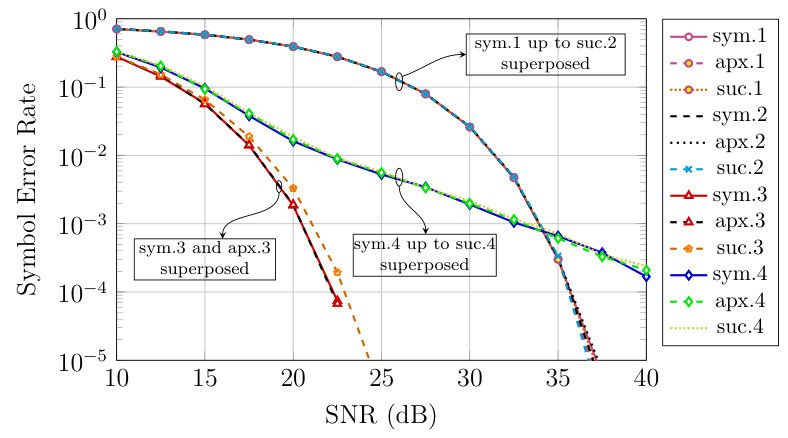 Figure 25
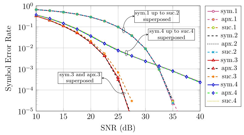 Figure 26
Peer Reviews
No public reviews on file for this paper yet. If you reviewed it on a platform where reviews are public (OpenReview, ICLR, NeurIPS, ICML), you can paste yours below so the community can read it here.
Videos
No videos yet. Explain this paper in a talk, walkthrough, or lecture? Add one.
Maximum Likelihood Detection in a Four-Dimensional
Stokes-Space Receiver
Amir Tasbihi and Frank R. Kschischang The authors are with the Edward S. Rogers Sr. Dept. of Electrical and Computer Engineering, University of Toronto, Toronto, ON M5S 3G4, Canada. Email: {tasbihi,frank}@ece.utoronto.ca. Submitted to IEEE Trans. Commun., February 1, 2019.
Abstract
The maximum likelihood detection rule for a four dimensional direct-detection optical front-end is derived. The four dimensions are two intensities and two differential phases. Three different signal processing algorithms, composed of symbol-by-symbol, sequence and successive detection, are discussed. To remedy dealing with special functions in the detection rules, an approximation for high signal-to-noise ratios (SNRs) is provided. Simulation results show that, despite the simpler structure of the successive algorithm, the resulting performance loss, in comparison with the other two algorithms, is negligible. For example, for an 8-ring/8-ary phase constellation, the complexity of detection reduces by a factor of 8, while the performance, in terms of the symbol error rate, degrades by 0.5 dB. It is shown that the high-SNR approximation is very accurate, even at low SNRs. The achievable rates for different constellations are computed and compared by the Monte Carlo method. For example, for a 4-ring/8-ary phase constellation, the achievable rate is 10 bits per channel use at an SNR of 25 dB, while by using an 8-ring/8-ary phase constellation and an error correcting code of rate 5/6, this rate is achieved at an SNR of 20 dB.
Index Terms:
Optical communication, non-coherent detection, Stokes space, maximum likelihood detection.
I Introduction
We derive the maximum likelihood (ML) detection rule for the four dimensional direct-detection receiver optical front-end described in [1]. We propose three digital signal processing (DSP) algorithms: symbol-by-symbol, sequence (min-sum) and successive detection. For each proposed method, we find the likelihood (utility) function to be maximized for the ML detection.
Due to their inexpensive structures, non-coherent detection schemes have promising applications in short-haul ( km) data transmission, e.g., intra data-center communication [2, 3]. In addition, the demand for high data rates necessitates the usage of all degrees of freedom (DOF) for data transmission.
Although exploiting the intensity or the phase of the transmitted light without using any local oscillator at the receiver was proposed earlier, exploiting both of them simultaneously in optical communication goes back to the early 2000s [4]. To combat the practical issue of precise adjustment in those techniques, self-homodyne detection was proposed in 2005 [5], which later was improved to exploit both of the polarizations for the data transmission in wavelength division multiplexing systems [6, 7]. Similar to self-homodyne detection, Stokes-vector direct detection (SVDD) was introduced in 2014, taking into account the polarization rotation of the fiber [3, 8]. Despite the simple structure of the receiver, SVDD (and also self-homodyne detection) devotes half of the available dimensions to the transmission of a pilot symbol. Later, a modified Stokes-space direct detection scheme was introduced in [1] which, by transmitting a data symbol instead of the pilot, achieves a higher data-rate. However, exploiting all of its DOF is only possible under either non-realistic assumptions or by using a complex receiver. This issue was later resolved for the same optical front-end by additional processing in the DSP [9]. The present paper extends the results of [9] by determining the actual ML detection rule for the various schemes under study.
The rest of the paper is organized as follows. The system model, including the transmitter, the channel and the receiver, is introduced in Sec. II. In Sec. III-A we discuss symbol-by-symbol ML detection. In Sec. III-B we describe sequence detection, exploiting the min-sum algorithm on the factor graph of the system. To combat the complexity of symbol-by-symbol and sequence detectors, we propose a successive detection scheme in Sec. III-C. Due to the existence of modified Bessel functions in the likelihood scores, we introduce an accurate and easy-to-compute approximation, suitable for operation in the moderate to large SNR regimes. These approximately ML decoders are described at the end of Secs. III-A, III-B, and III-C. In Sec. IV, we discuss about the fast fading behaviour of the fourth DOF subchannel. In Sec. V, we compare the discussed methods in previous sections via simulations. Finally, we provide concluding remarks in Sec. VI.
Through this paper, we adopt the following notational conventions.
- •
Scalars: lower-case letters, e.g., and .
- •
: the magnitude, phase, real and imaginary parts and complex conjugate of the complex number , respectively.
- •
Sets: blackboard bold capital letters, e.g., . In particular, , , and denote integers, real numbers, non-negative reals, and complex numbers, respectively.
- •
↔ : there is a bijection between and .
- •
Vectors: lower-case bold letters, e.g., . The element of is denoted by . For , the inner product is defined as
- •
Matrices: upper-case bold letters, e.g., . In addition, denotes the identity matrix.
- •
and : the determinant and the transpose of .
- •
Random variables: non-bold capital letters, e.g. . Realizations are shown in the same lower-case letter, e.g., if is a random variable then is its realization.
- •
: the sequence , where .
- •
: the unit-delay operator, e.g., if denotes a discrete-time signal then .
- •
We will extensively make use of the Jones vector representation of light [10]. For the Jones vector , and denote the X and Y polarizations, respectively.
II The System Model
In this section, we formulate the signal processing operations performed by the transmitter, the channel, and the receiver.
II-A The Transmitter
For simplicity, we discuss the base-band equivalent model. We assume the use of Nyquist pulses, i.e., pulses without intersymbol interference, allowing for a discrete-time formulation corresponding to the sample times. We use an -ring/-ary phase constellation (See Fig. 1) with equally-spaced squared radii as in [1]. The radius set is
[TABLE]
where and , and the phase set is
[TABLE]
The transmitter sends two points, and , from the constellation over the X and Y polarizations, respectively. As a result, the transmitted symbol is . As and are complex numbers, they have a magnitude and a phase, providing four DOF to exploit. As with any non-coherent scheme, instead of the absolute phase, we use differential phase encoding. As a result, we encode our data in
- i)
, 2. ii)
, 3. iii)
, 4. iv)
,
which we refer to as the first up to the fourth dimension, respectively. The relationship among these dimensions are shown in Fig. 2a. The fourth dimension necessitates an initial condition on a symbol block, which is achieved by transmitting a pilot symbol, e.g., , at the beginning of the block.
II-B The Channel
We adopt a linear channel model, neglecting fiber nonlinearities, as is appropriate for short-haul data transmission. The random birefringence of single mode fibers impose a linear transformation on the input Jones vector. In particular, in the absence of noise, the output Jones vector, , can be written as
[TABLE]
where
[TABLE]
is the channel rotation matrix, such that and [11, 12, 13, 1]. The matrix is nonsingular; so if and denote all possible and vectors, respectively, then ↔. The coherence time of the channel matrix is assumed to be much larger than a symbol duration, so we can neglect its variation over the transmission of a sequence of symbols. Fiber loss is not considered in (1), as it is compensated by a receiver amplifier. The amplifier contaminates with amplified spontaneous emission noise, , which is a zero-mean additive white Gaussian noise with the covariance matrix [10]. Its output is , hence
[TABLE]
The angles and are defined in the same way as their “-domain counterparts” as
[TABLE]
as shown in Figs. 2b and 2c. The relation among and is shown in Fig. 3. It is assumed that the receiver knows the channel parameters, i.e., and ; such knowledge can be attained by transmitting training symbols at the beginning of data blocks [8].
II-C The Optical Front-end
We use the same optical front-end as proposed in [1] and shown in Fig. 4. Its components are:
- •
polarization beam splitter (PBS), which splits the input Jones vector into its and polarizations;
- •
photo-diode (PD), which transforms its input, , to its output, ;
- •
balanced photo-detector (BPD), which transform its two inputs, and , to its output, ;
- •
optical hybrid, which transforms its two inputs, and , to its four outputs, .
The outputs of the optical front-end, , are six real-valued numbers which are processed in the back-end DSP to detect , denoted by (see Fig. 3). The relation between and is [9]
[TABLE]
III ML Detection
In this section, we derive the ML detector for the transmitted data under three processing assumptions, after observing . Based on the transmitted and the received quantities, we define the vectors
[TABLE]
and
[TABLE]
Note that and are in one-to-one correspondence. The relationship among , and the components of and is depicted in Fig. 5, to be used in later sections.
III-A Symbol-by-symbol ML Detection
In this section, we discuss about the symbol-by-symbol detection of all four dimensions. As ↔, for the ease of computation, first we decide on ; after that, by a bijection we find . In this process is fixed as it is decoded in the previous time slot.
By the definition of conditional PDF, we can write the likelihood function as
[TABLE]
In Theorems 1 and 2, we find and , respectively. After that, we can find the likelihood function by (5).
Theorem 1**.**
[TABLE]
where denotes the modified Bessel function of order zero and for .
Proof.
Let and be the random variables representing the received and the transmitted (in domain) signals. Note that and are independent complex Gaussian random variables, with means and each one has a covariance matrix . The radius has a Rician distribution with the PDF given as [14]
[TABLE]
In addition, given , is independent of other parameters in , so we have
[TABLE]
from which (6) is obtained by substituting from (7). ∎
Theorem 2**.**
[TABLE]
Proof.
See Appendix A. ∎
By using Theorems 1 and 2, and (5), we have
[TABLE]
Note that is the magnitude of the correlation of the observation, , and the hypothesis, (see Fig. 5.)
To do ML symbol-by-symbol detection, we must solve
[TABLE]
From (4), we see that given , there is a bijection between and , which allows us to rewrite (9) as
[TABLE]
Noting that is constant, by (8) and eliminating the common factors among all hypotheses, (10) is equivalent to
[TABLE]
which in practice can be solved by examining all possible ’s that satisfy the condition.
After finding from (11), we find the equivalent . Note that [1]
[TABLE]
where
[TABLE]
Hence, after decoding , by using (12) we can find . To decide on , we note that [9]
[TABLE]
where
[TABLE]
After decoding from (11) and finding from (12), the only unknown in (13) is , which can easily be solved for.
High SNR approximation
For large arguments, can be approximated as [15, eq. 9.7.1]
[TABLE]
By neglecting terms in (14) and noting that
[TABLE]
we can approximate (11) at high SNRs as
[TABLE]
Despite the “similarity” of (16) and the minimum-distance decoder, they behave differently. By eliminating in the expansion of , the minimum-distance decoder solves
[TABLE]
which is different from (16). For example, for , , , we have
[TABLE]
while
[TABLE]
As a result, the minimum-distance decoder maps to , while the ML decoder maps it to .
III-B Sequence ML Detection
In this section, we show how to decode a sequence of transmitted data by using the min-sum algorithm on the factor-graph of the system [16]. The sequence comprises two types of symbols: a pilot symbol which is sent at the beginning of the sequence, and is known to the receiver (see Sec. II-A), and data symbols.
The flow-graph of the system for a sequence of length four is shown at Fig. 6. Variable nodes (v-nodes) and check nodes (c-nodes) are shown with circles and rectangles respectively. The channel matrix is represented by and the optical front-end is denoted by .
Solving ML sequence-detection (MLSD) problem requires finding
[TABLE]
which, as ↔, can be written as
[TABLE]
where and are the pilot symbols. Note that and form a second-order hidden Markov chain and as a result
[TABLE]
By using (8), (17) is equivalent to
[TABLE]
which suggests to use the min-sum algorithm on its factor graph. A factor-graph representation of the objective function of (18) for a sequence of length four is shown in Fig. 7. Note that the factor graph is cycle-free, hence the min-sum algorithm produces the exact minimum. In addition, it is equivalent to the Viterbi algorithm [16].
High SNR approximation
From (14) and (15), (18) can be approximated at high SNRs as
[TABLE]
III-C Successive ML Detection
In symbol-by-symbol detection, we search over all possible transmitted symbols for the detection of each received symbol; e.g., for an -ring/-ary phase constellation for each polarization, different possibilities must be examined. We can reduce this complexity by decoding in a successive manner, at the expense of an increase in SER. In the proposed successive detection method, we decode the first three dimensions jointly, then proceed to decode the fourth one with the knowledge of the first three dimensions. In this way, we must examine different possibilities; which, for a large value of , the complexity reduction is significant. For example, for an -ring/-ary phase constellation, we must search over possibilities to decode each symbol in the symbol-by-symbol scheme, while this number reduces to for successive detection.
III-C1 The Likelihood Function at the First Successive-Step
The ML detection of the first three dimensions necessitates solving
[TABLE]
which, due to the bijection between and (see (4)), can be written as
[TABLE]
In Theorem 3, we find the likelihood function of the first three dimensions.
Theorem 3**.**
[TABLE]
Proof.
See Appendix B. ∎
By using Theorem 3, we can rewrite (19) as
[TABLE]
Note that the optimal , obtained by solving (20), is the closest possible one to , i.e., it maximizes over all feasible . That is because and are strictly increasing functions. Hence, to minimize the objective function of (20), we must maximize , which from Fig. 5 obtains when is the “closest” one to zero, i.e., must be maximized.
High SNR approximation
Similar to the symbol-by-symbol detection, at high SNRs, (20) can be approximated as
[TABLE]
III-C2 The Second Successive-Step
At the second successive-step, the fourth dimension is decoded. According to (4) we have
[TABLE]
At this step, the intensities are treated as constants, as they have been decoded at the first successive-step. As a result, there is a bijection between and . The decoder performs ML detection of by solving
[TABLE]
Theorem 4 provides an easy way to decide on .
Theorem 4**.**
[TABLE]
where , as shown in Fig. 5.
Proof.
See Appendix C. ∎
The interpretation of (22) is that the decoder chooses the closest feasible to . This can be justified by using Fig. 5 and (11) as well. In the first successive step we have decoded and as a result, are fixed. From (11), we must maximize to minimize its objective function, which happens when the segment in Fig. 5 has the smallest angular deviation from the segment . This means that must be the closest one to .
IV Subchannel Fading
In this section, we show that the optical front-end, studied in this paper, causes the fourth DOF () to be subjected to fast fading, which makes this subchannel exhibit a symbol error rate behaviour that is markedly different than the other subchannels. For the purpose of this discussion, we neglect the effect of noise (setting noise to zero); instead, we focus on the effect that the channel matrix, , has on the four DOF subchannels.
As we see from (12), the relationship between the input and the output of the first three DOF subchannels is determined by , and does not depend on previously transmitted symbols. As a result, the subchannels of the first three dimensions change only block-by-block; hence, we expect the first three dimensions to experience a slow (block) fading channel.
The output of the fourth subchannel, however, is not only a function of the channel parameters, but also a function of the previously transmitted symbols as well. Particularly, from (13), we have
[TABLE]
where, the complex number is
[TABLE]
The coefficient is a function of , which makes the fourth DOF subchannel vary symbol-by-symbol. As a result, we see that the fourth DOF subchannel suffers from fast fading; and similar to a Rayleigh fading channel, we expect the symbol error rate of the fourth dimension to be proportional to [17, p. 533]. In Sec. V, we see that the SER figures support this claim.
V Numerical Results
In this section, we provide some numerical results to compare the discussed detection methods. For all figures, the SNR is defined as the average transmitted energy per polarization over the complex-noise variance per polarization. Specifically, for the discussed constellation, the SNR is defined as
[TABLE]
The resulting SERs for different constellations are shown in Figs. 8–14. The channel matrix for each block of data is chosen uniformly over all possible matrices (see Sec. II-B). By increasing , the rings become more distant from each other, hence it improves the performance of the first two dimensions in terms of SER, but there is a trade-off with the performance of the phase channels. For example, for -ring/-ary phase constellation and the target SER of , changing from to results an improve of dB in the intensity channels, while it degrades the performance of the third channel by dB (compare Figs. 8 and 9). As another example, for -ring/-ary phase constellation and the same target SER, by changing from to , the performance of the first two dimensions improve by dB, while the performance of the third and the fourth dimensions degrades by dB and dB, respectively (compare Figs. 10–12).
As shown, while the complexity of successive detection is smaller than other methods, its SER does not differ noticeably. For example, by using -ring/-ary phase constellation with successive detection, the complexity of brute-force search is reduced (approximately) by a factor of 8, while for the target SER of , it degrades the performance of the third channel less than dB for , and does not affect the performance of other dimensions noticeably (see Fig. 10).
From Figs. 8–12, we see that the high-SNR approximation is a very good approximation which, by avoiding computing the modified Bessel function, can reduce the complexity of decoder. In all of these figures, the approximated figures and the actual ones are almost superposed. As a result, due to the large size of the constellation and to remedy the long running time of the simulation, the SER figures for -ring/-ary phase constellation are computed by high-SNR approximated formula.
As discussed in Sec. IV, we expect the fourth dimension to be under fast fading. The results support our expectation. Similar to a Rayleigh fading channel, the SER of the fourth dimension is proportional to , and that is the reason of the linear behaviour of the fourth dimension symbol error rate, shown in Figs. 8–14. The fast fading behaviour is due to the non-zero entry in the matrix, which entangles the fourth channel with the past data. Hence, we expect the fourth dimension to behave as same as the third dimension when . Fig. 15 shows that this is indeed true. For this figure, the channel matrix varies block-by-block, but in all cases, its entry is zero. As , the no-entanglement condition implies that , for some random .
The achievable rate for different constellations and are shown in Figs. 16–19. The rates are actually
[TABLE]
where denotes the mutual information between the random variables and , and is computed by the Monte Carlo method. As there is a conditioning on , (23) is actually the achievable rate of the scheme, where the receiver feeds back the intensity of the received Y polarization. As we are using an -ring/-ary phase constellation, the maximum rate is bits per channel use.
The which causes the minimum Euclidean distance between two points on a ring (which happens for the inner-most ring) to be the same as the minimum Euclidean distance between two points on different rings (which happens for the two outer-most rings) is denoted by (balanced ). It can be easily shown that
[TABLE]
As it is shown in Figs. 16–19, although is not the optimal , it is nearly optimal. The for different constellation are shown in Table I. Inspired by [18], in Fig. 20 we have compared the achievable rate of different constellations at their . This figure shows the necessity of using an error-correcting code at the encoder. For example, by using a 4-ring/8-ary phase constellation without any error-correcting code, we can transmit bits per channel use at the SNR of dB, while by using an 8-ring/8-ary phase constellation and a code of rate , we can achieve the same rate at the SNR of dB; hence, we can save dB.
VI Conclusion
We computed the maximum likelihood detection rule for symbol-by-symbol and sequence decoding, in a four-dimensional Stokes-space scheme. To reduce the complexity of those schemes, we introduced a successive detection method. To remedy dealing with special functions, we provided a high-SNR approximation of the detection rules as well. We saw that the optical front-end studied in this paper subjects the subchannel of one of the dimensions to fast fading. The decoding methods are compared by simulations. We saw that using the successive method results a negligible loss, and in addition, the high-SNR approximation is very accurate (even at low SNRs). Furthermore, the achievable rates of different constellations are obtained by the Monte Carlo method.
An interesting future problem would be to design a a good error correcting code and modulation, specialized for a particular application. We have assumed that noise contaminates the signal in the optical domain, while a more comprehensive model might be to consider an additive noise source in the electrical domain (after the photo diodes) as well. In that model, a noise term must be added to each of the six output values, . Determing the ML detection rule for that scheme is left as future research. Throughout this paper, we assumed that the receiver perfectly knows the channel matrix; it would be interesting to conduct an analysis to determine how sensitive the detection performance is to this assumption.
Appendix A
Proof of Theorem 2.
The phase of , , has a von Mises distribution with the PDF given as [19]
[TABLE]
Note that
[TABLE]
and as a result, and are functions of and . Therefore, we use the Jacobian of this transformation to compute the joint conditional PDF of and from the joint conditional PDF of and [20, p. 244]. To use the Jacobian, the number of random variables before and after the transformation must be the same, which is not true in this case. We introduce a dummy random variable, , and find the joint conditional PDF of , and . Then by marginalizing , we obtain the PDF of interest.
The determinant of the Jacobian matrix is
[TABLE]
where, e.g., the element in the first row and the second column of the Jacobian matrix is . As there is a one-to-one correspondence between and , there is only a unique that contributes to the PDF of . Let denote the condition vector. Then we have
[TABLE]
where is due to the independence of and , and is true as, by using Fig. 5, we have
[TABLE]
As a result,
[TABLE]
By marginalizing , we have
[TABLE]
where in , we have ignored the constant phase offset, , as we are integrating over one period of cosine function. ∎
Appendix B
Proof of Theorem 3.
We adopt the proof given in [19], with some adaptation to be consistent with our notation. Let . By the definition of conditional PDF, we have
[TABLE]
so, to find , we compute and .
As said in the proof of Theorem 1, given , becomes independent of , for . As a result, according to Theorem 1, we have
[TABLE]
To compute , note that is the subtraction of two independent von Mises random variables (see (27).) As a result, its PDF is the convolution of two von Mises PDFs, given as
[TABLE]
where is true as
[TABLE]
and for see Fig. 5 [21, p. 44]. Using (28) and (29), we have
[TABLE]
∎
Appendix C
Proof of Theorem 4.
Given , becomes independent of . As a result, we have
[TABLE]
where is true due to (8) and Theorem 3, and is true as, at this step, is the same for all feasible . ∎
The reference list from the paper itself. Each links out to its DOI / PubMed record.
- 1[1] M. Morsy-Osman, M. Chagnon, and D. V. Plant, “Four-dimensional modulation and Stokes direct detection of polarization division multiplexed intensities, inter polarization phase and inter polarization differential phase,” J. Lightwave Techn. , vol. 34, no. 7, pp. 1585–1592, Apr. 2016.
- 2[2] S. Aleksic, “The future of optical interconnects for data centers: A review of technology trends,” in Int. Conf. on Telecommun. (Con TEL) , Jun. 2017, pp. 41–46.
- 3[3] D. Che, A. Li, X. Chen, Q. Hu, Y. Wang, and W. Shieh, “160-Gb/s Stokes vector direct detection for short reach optical communication,” in Opt. Fiber Commun. Conf. and Exh. (OFC) , Mar. 2014, pp. (Th 5C.7)1–3.
- 4[4] M. Ohm and J. Speidel, “Quaternary optical ASK-DPSK and receivers with direct detection,” IEEE Photon. Technol. Lett. , vol. 15, no. 1, pp. 159–161, Jan. 2003.
- 5[5] T. Miyazaki and F. Kubota, “PSK self-homodyne detection using a pilot carrier for multibit/symbol transmission with inverse-RZ signal,” IEEE Photon. Technol. Lett. , vol. 17, no. 6, pp. 1334–1336, Jun. 2005.
- 6[6] M. Sjödin, E. Agrell, G. W. Lu, P. Johannisson, M. Karlsson, and P. Andrekson, “Interleaved polarization division multiplexing in self-homodyne coherent WDM systems,” in Europ. Conf. Opt. Commn. (ECOC) , Sep. 2010, pp. (Mo.1.C.3)1–3.
- 7[7] M. Sjödin, E. Agrell, P. Johannisson, G. W. Lu, P. A. Andrekson, and M. Karlsson, “Filter optimization for self-homodyne coherent WDM systems using interleaved polarization division multiplexing,” J. Lightwave Techn. , vol. 29, no. 9, pp. 1219–1226, May 2011.
- 8[8] D. Che, A. Li, X. Chen, Q. Hu, Y. Wang, and W. Shieh, “Stokes vector direct detection for linear complex optical channels,” J. Lightwave Techn. , vol. 33, no. 3, pp. 678–684, Feb. 2015.