Public decision support for low population density areas: An imbalance-aware hyper-ensemble for spatio-temporal crime prediction
Cristina Kadar, Rudolf Maculan, Stefan Feuerriegel

TL;DR
This paper introduces an imbalance-aware hyper-ensemble machine learning approach for predicting crime hotspots in low population density areas, significantly improving detection accuracy despite data sparsity.
Contribution
It presents a novel hyper-ensemble model specifically designed to handle class imbalance in spatio-temporal crime prediction in low-density regions.
Findings
Hit ratio increased from 18.1% to 24.6% for top 5% hotspots.
Hit ratio increased from 53.1% to 60.4% for top 20% hotspots.
Model outperforms state-of-the-art predictors in imbalanced settings.
Abstract
Crime events are known to reveal spatio-temporal patterns, which can be used for predictive modeling and subsequent decision support. While the focus has hitherto been placed on areas with high population density, we address the challenging undertaking of predicting crime hotspots in regions with low population densities and highly unequally-distributed crime.This results in a severe sparsity (i.e., class imbalance) of the outcome variable, which impedes predictive modeling. To alleviate this, we develop machine learning models for spatio-temporal prediction that are specifically adjusted for an imbalanced distribution of the class labels and test them in an actual setting with state-of-the-art predictors (i.e., socio-economic, geographical, temporal, meteorological, and crime variables in fine resolution). The proposed imbalance-aware hyper-ensemble increases the hit ratio considerably…
Click any figure to enlarge with its caption.
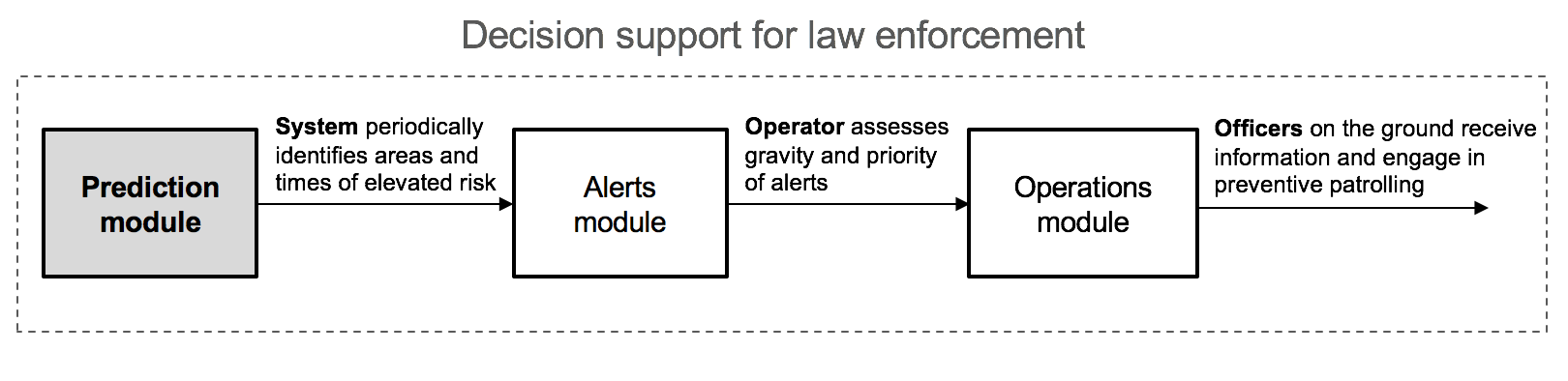 Figure 1
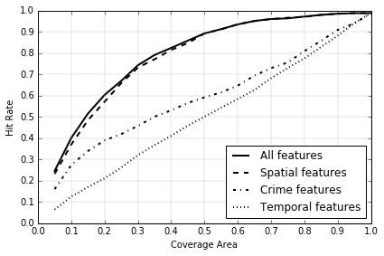 Figure 2
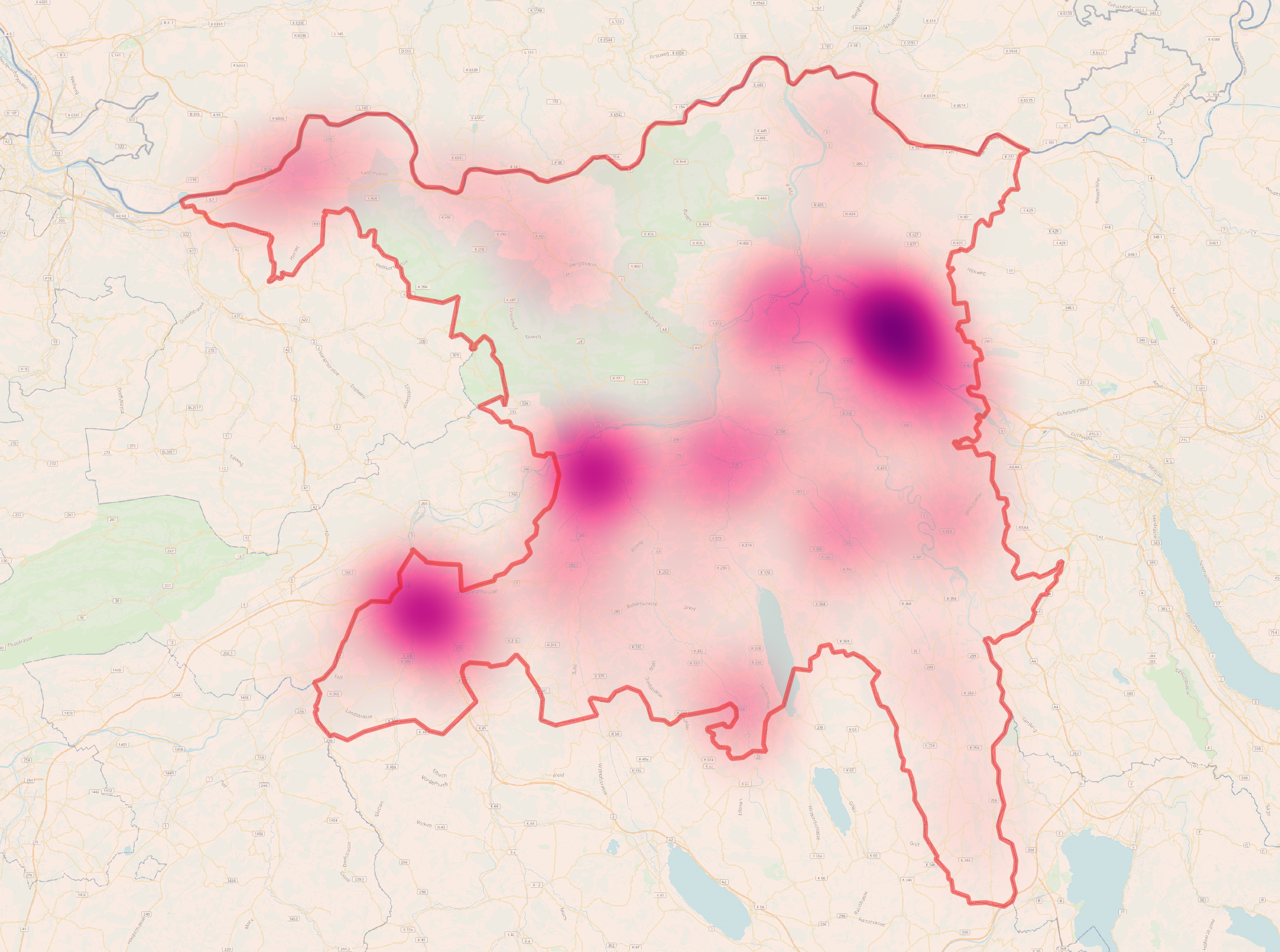 Figure 3
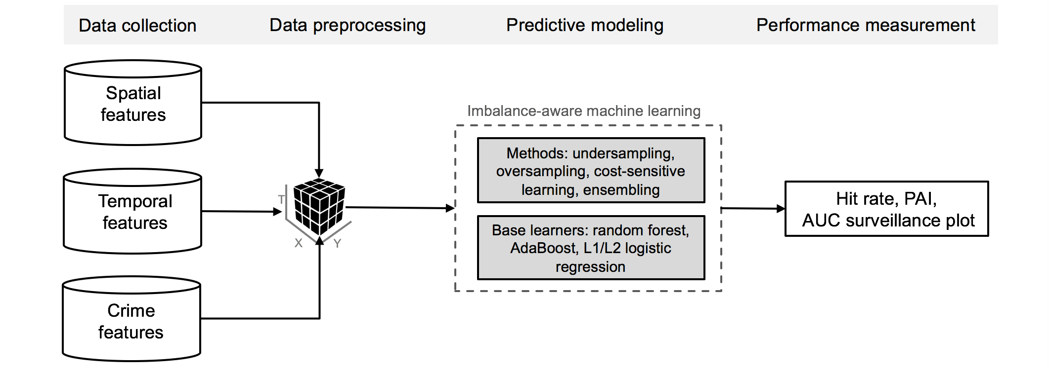 Figure 4
| Study | Population density | Study area | Spatial resolution | Temporal resolution | Features | Method |
| Bowers et al. [2004] | High | Liverpool | Grid cells of 50 m 50 m | 2 days / 1 week | Crime | Prospective hotspot |
| Mohler et al. [2011] | High | Part of Los Angeles | Grid cells of 200 m 200 m | 1 day | Crime | Self-exciting point processes |
| Wang & Brown [2012] | High | Charlottesville | Grid cells of 32 m 32 m | 1 month | Crime, spatial | Spatio-temporal generalized additive model |
| Gerber [2014] | High | Los Angeles | Points at 200 m 200 m intervals | 1 day | Crime, social media | Logistic regression |
| Bogomolov et al. [2014] | High | London metropolitan area | Lower layer super output areas (geographic hierarchy) | 1 month | Crime, spatial, telecom | Random forest |
| Rummens et al. [2017] | High | Unnamed city in Belgium | Grid cells of 200 m 200 m | 2 weeks | Crime, spatial, temporal | Logistic regression, neural network |
| Vomfell et al. [2018] | High | New York City | \pbox6cmCensus tracts | |||
| (geographic hierarchy) | 1 week | Crime, spatial, social media, mobility | Random forest, gradient boosting, neural network | |||
| This work | Low | Swiss canton Aargau (analogous to an US state) | Grid cells of 200 m 200 m | 1 day | Crime, spatial, temporal | Hyper-ensemble |
| Type | Theory | Name | Dimension | Description | Source |
| Crime | (Near) repeat victimization | prior1d, prior3d, prior7d, prior14d | integer | Number of offenses in the respective and neighboring cells in the past days | Aargau cantonal police |
| Locational | Social disorganization theory | popdens | people/hectare | Density of total residential population | AGIS: “Statistik der Bevoelkerung auf Hektarbasis” |
| popbirth_nonCH | percent | Fraction of residents not born in Switzerland | |||
| popcit_EU, popcit_europ, popcit_noneurop, popcit_CH | percent | Fraction of residents: EU, non-EU European, non-European, or Swiss citizens | |||
| popcit_dividx | real between 0 and 1 | Diversity121212Diversity is computed as the normalized Shannon entropy, given all possible categories for the variable, similarly to the approach in Kadar & Pletikosa [2018]. The resulting value lies between 0 (homogenous) and 1 (diverse). of citizenship. | |||
| pop_age1, pop_age2, pop_age3, pop_age4 | percent | Fraction of residents between 0-19, 20-34, 35-64 and 65+ years of age | |||
| popage_dividx | real between 0 and 1 | Diversity of age | |||
| popmale | percent | Fraction of male residential population | |||
| popstab | percent | Fraction of stable residential population | |||
| busidens | businesses/hectare | Density of workplaces | AGIS: “Statistik der Unternehmensstruktur (STATENT) 2013 auf Hektarbasis” | ||
| busi_sec1, busi_sec2, busi_sec3 | percent | Fraction of businesses in sectors 1, 2 and 3 | |||
| busisec_dividx | real between 0 and 1 | Diversity of workplaces with respect to sector | |||
| emplsec_dividx | real between 0 and 1 | Diversity of employees with respect to sector | |||
| empldens | employees/hectare | Density of employees | |||
| emplmale | percent | Fraction of male employees | |||
| Crime pattern theory | land_indust, land_park, land_resi1, … | percent | Fraction of land usage: industry, park, residential area with 1 story buildings, … | AGIS: “Bauzonen Schweiz (harmonisiert) Ausschnitt AG gemaess MGDM” | |
| land_dividx | real between 0 and 1 | Diversity of land use | |||
| buildgs_areafrac | percent | Fraction of area within a grid cell covered by buildings | AGIS: “Gebaeude ab Uebersichtsplan 1_5000” | ||
| buildgs_dens | buildings/hectare | Density of buildings within a grid cell | |||
| poi_infra | points/hectare | Density of infrastructural items such as ATMs, post boxes, waste baskets, etc. | OpenStreetMap Switzerland | ||
| poi_shop | points/hectare | Density of shops | |||
| poi_public | points/hectare | Density of public buildings such as police stations, hospitals, etc. | |||
| poi_edu | points/hectare | Density of educational institutions such as schools, kindergartens, etc. | |||
| poi_gastro | points/hectare | Density of gastronomical amenities such as restaurants, bars, etc. | |||
| pub_hous | boolean | Occurrence of a public housing unit in a grid cell | Bundesamt fuer Wohnungswesen | ||
| highway_exits | boolean | Occurrence of a highway exit within 5,000 m of the grid cell | AGIS: “Netz Kantons- strassen und Nationalstrassen” | ||
| border_cross | boolean | Occurrence of a border crossing within 5,000 m of the grid cell | |||
| road_type | category | Type of a road in the grid cell: from 0 = no road to 3 = high volume road | |||
| intersection | boolean | Occurrence of a major crossroads in the respective or neighboring grid cells | |||
| pub_trans | real between 0 and 1 | Quality measure for public transport | AGIS: “OeV Gueteklassen” | ||
| Temporal | Climatic and seasonal | dow | encoded | The day of the week | — |
| holiday | boolean | Indicator of whether there is a public holiday | feiertagskalender.ch | ||
| temp | degree celsius | Temperature at 12 am | Darksky API | ||
| hum | percent | Humidity at 12 am | |||
| discomf | real | Discomfort index | |||
| daylight | hours | Hours of daylight | |||
| moon | float between 0 and 1 | Moon phase (1 = full moon) | |||
| event | integer | Number of public events on the specific day for the respective cell | events.ch |
| Classifier | 5 % Coverage area | 10 % Coverage area | 20 % Coverage area | AUC | |||
| Hit rate | PAI | Hit rate | PAI | Hit rate | PAI | ||
| Majority class classifier | 0.0 % | 0.000 | 0.0 % | 0.000 | 0.0 % | 0.000 | 0.000 |
| Naïve classifier | 18.1 % | 3.621 | 32.5 % | 3.249 | 53.0 % | 2.651 | 0.754 |
| Cost-sensitive learning | 21.0 % | 4.186 | 36.1 % | 3.611 | 58.7 % | 2.935 | |
| Random over-sampling | 15.5 % | 3.094 | 25.2 % | 2.523 | 40.8 % | 2.040 | 0.593 |
| Random under-sampling | 23.3 % | 4.665 | 38.4 % | 3.840 | 59.1 % | 2.953 | 0.773 |
| Heuristic over-sampling | 16.2 % | 3.252 | 26.5 % | 2.649 | 41.3 % | 2.063 | 0.590 |
| Heuristic under-sampling | 12.5 % | 2.495 | 21.8 % | 2.181 | 43.2 % | 2.159 | 0.721 |
| Hyper-ensemble | 24.6 % | 4.932 | 40.2 % | 4.020 | 60.4 % | 3.021 | 0.779 |
| Classifier | Base learner | 5 % Coverage area | 10 % Coverage area | 20 % Coverage area | AUC | |||
| Hit rate | PAI | Hit rate | PAI | Hit rate | PAI | |||
| Random under-sampling | Random forest | 23.3 % | 4.665 | 38.4 % | 3.840 | 59.1 % | 2.952 | 0.773 |
| Random under-sampling | AdaBoost | 23.2 % | 4.654 | 37.7 % | 3.771 | 58.7 % | 2.933 | 0.771 |
| Random under-sampling | L2 logistic regression | 24.6 % | 4.922 | 37.1 % | 3.712 | 57.3 % | 2.866 | 0.768 |
| Random under-sampling | L1 logistic regression | 21.8 % | 4.363 | 34.1 % | 3.407 | 54.4 % | 2.717 | 0.758 |
| Hyper-ensemble | Random forest | 24.6 % | 4.932 | 40.2 % | 4.020 | 60.4 % | 3.021 | 0.779 |
| Hyper-ensemble | AdaBoost | 23.3 % | 4.659 | 38.1 % | 3.809 | 59.2 % | 2.959 | 0.772 |
| Hyper-ensemble | L2 logistic regression | 24.7 % | 4.936 | 37.3 % | 3.731 | 57.4 % | 2.868 | 0.769 |
| Hyper-ensemble | L1 logistic regression | 22.1 % | 4.414 | 34.1 % | 3.409 | 54.5 % | 2.722 | 0.758 |
| Population density | Feature set | 5 % Coverage area | 10 % Coverage area | 20 % Coverage area | AUC | |||
| Hit rate | PAI | Hit rate | PAI | Hit rate | PAI | |||
| All | Crime | 16.1 % | 3.213 | 27.4 % | 2.743 | 39.0 % | 1.949 | 0.581 |
| Temporal | 6.5 % | 1.292 | 12.5 % | 1.255 | 21.1 % | 1.057 | 0.498 | |
| Spatial | 23.3 % | 4.655 | 37.1 % | 3.711 | 57.2 % | 2.860 | 0.771 | |
| All | 24.6 % | 4.932 | 40.2 % | 4.020 | 60.4 % | 3.021 | 0.779 | |
| Low population density | Crime | 4.0 % | 0.813 | 5.0 % | 0.508 | 8.0 % | 0.402 | 0.157 |
| Temporal | 0.7 % | 0.142 | 3.8 % | 0.385 | 6.5 % | 0.324 | 0.154 | |
| Spatial | 10.5 % | 2.096 | 15.7 % | 1.568 | 21.2 % | 1.060 | 0.251 | |
| All | 10.5 % | 2.096 | 15.7 % | 1.568 | 21.2 % | 1.060 | 0.251 | |
| Medium population density | Crime | 8.4 % | 1.686 | 13.6 % | 1.357 | 20.4 % | 1.019 | 0.355 |
| Temporal | 3.1 % | 0.623 | 7.6 % | 0.763 | 14.5 % | 0.726 | 0.327 | |
| Spatial | 14.0 % | 2.805 | 20.4 % | 2.043 | 31.5 % | 1.572 | 0.447 | |
| All | 15.6 % | 3.123 | 21.5 % | 2.156 | 29.9 % | 1.493 | 0.448 | |
| High population density | Crime | 11.6 % | 2.320 | 21.9 % | 2.185 | 35.1 % | 1.756 | 0.561 |
| Temporal | 6.0 % | 1.199 | 11.3 % | 1.132 | 21.7 % | 1.083 | 0.486 | |
| Spatial | 15.1 % | 3.033 | 23.5 % | 2.348 | 39.2 % | 1.960 | 0.633 | |
| All | 15.0 % | 3.013 | 27.2 % | 2.721 | 41.8 % | 2.091 | 0.651 | |
Peer Reviews
No public reviews on file for this paper yet. If you reviewed it on a platform where reviews are public (OpenReview, ICLR, NeurIPS, ICML), you can paste yours below so the community can read it here.
Videos
No videos yet. Explain this paper in a talk, walkthrough, or lecture? Add one.
Taxonomy
TopicsCrime Patterns and Interventions · Data-Driven Disease Surveillance · Gambling Behavior and Treatments
Public decision support for low population density areas: An imbalance-aware hyper-ensemble for spatio-temporal crime prediction
Cristina Kadar111These authors contributed equally to this work and are listed alphabetically.
Rudolf Maculan222These authors contributed equally to this work and are listed alphabetically.
Stefan Feuerriegel
ETH Zurich, Weinbergstr. 56/58, 8092 Zurich, Switzerland
Abstract
Crime events are known to reveal spatio-temporal patterns, which can be used for predictive modeling and subsequent decision support. While the focus has hitherto been placed on areas with high population density, we address the challenging undertaking of predicting crime hotspots in regions with low population densities and highly unequally-distributed crime.This results in a severe sparsity (i. e., class imbalance) of the outcome variable, which impedes predictive modeling. To alleviate this, we develop machine learning models for spatio-temporal prediction that are specifically adjusted for an imbalanced distribution of the class labels and test them in an actual setting with state-of-the-art predictors (i. e., socio-economic, geographical, temporal, meteorological, and crime variables in fine resolution). The proposed imbalance-aware hyper-ensemble increases the hit ratio considerably from to when aiming for the top of hotspots, and from to when aiming for the top of hotspots. As direct implications, the findings help decision-makers in law enforcement and contribute to public decision support in low population density regions.
keywords:
Crime prediction , Machine learning , Imbalanced data , Spatio-temporal modeling , Public decision support
††journal: arXiv
1 Introduction
Crime inflicts immense financial losses upon individuals, businesses, and organizations, and can even threaten the stability of societies. For instance, according to recent figures from the Federal Bureau of Investigation, annual financial losses due to property crime in the United States amount to 3.6 bn USD, with an average cost of 2,361 USD per burglary.333US Federal Bureau of Investigation, Uniform crime report: https://ucr.fbi.gov/crime-in-the-u.s/2016/crime-in-the-u.s.-2016/topic-pages/burglary. Last accessed: March 11, 2018. Beyond the financial damage, crime incidents are also known to trigger negative social and psychological effects, since victims suffer from a heightened level of perceived risk, which has been found to result in a significant decrease in the quality of life [Doran & Burgess, 2012]. Hence, it is the objective of decision-makers in the private and public sectors to find strategies for effective crime prevention.
In the effort to reduce crime, governments and law enforcement agencies, such as US police departments, have recently started experimenting with techniques for predictive policing in order to optimize the use of resources and to increase the chances of deterring, as well as preventing, crime events.444US Federal Bureau of Investigation, Articles: https://leb.fbi.gov/articles/featured-articles/predictive-policing-using-technology-to-reduce-crime. Last accessed: August 4, 2018. The term “predictive policing” refers to the use of predictive analytics with the aim of identifying the potential location of criminal activity prior to such an event taking place [Ratcliffe, 2014]. Formally, this approach draws upon historical records of crime events in order to make spatio-temporal forecasts [Bowers et al., 2004, Mohler et al., 2011].555We point out that, throughout this work, we build upon the place-centric notion of crime prediction, with the aim of forecasting time-dependent spatial hot spots of elevated crime risk. This is in contrast to a people-centric notion, such as adopted by Canter et al. [2000] or Wang et al. [2013], which aims at identifying attributes of potential offenders. In addition, the predictive models are often extended by further information related to the socio-economic status of the resident population and to nearby points of interest (POI) [Kadar et al., 2017, Rummens et al., 2017, Vomfell et al., 2018, Wang & Brown, 2012, Xue & Brown, 2006], basic temporal variables [Rummens et al., 2017, Wang & Brown, 2012], or even social media, telecom, or mobility data [Bogomolov et al., 2014, Gerber, 2014, Kadar & Pletikosa, 2018, Vomfell et al., 2018, Wang et al., 2016], in order to better adapt to the spatio-temporal nature of crime events.
Forecasts from predictive policing improve situational awareness at both the tactical and strategic levels for law enforcement bodies and help them develop strategies for more efficient and effective policing [Perry et al., 2013, p. 2]. Figure 1 summarizes the main steps involved in deriving tactical decision support from predictive policing. In doing so, predictive policing is based on the assumption that the presence of police offers at crime hotspots leads to decreasing crime rates, which has been recently validated in randomized controlled trials [Mohler et al., 2015].
Previous research has developed models for crime prediction that target highly populated areas. Examples include cities such as Los Angeles [Gerber, 2014], London [Bogomolov et al., 2014], and Liverpool [Bowers et al., 2004]. Other studies even narrow the focus to individual districts such as the San Fernando Valley in Los Angeles [Mohler et al., 2011]. Yet there is scant evidence that predictive policing can also be applied to areas with lower population density. In fact, prior literature has overlooked sparsely-populated regions, despite the fact that over 50 percent of household burglaries in the US occur in such areas.666Bureau of Justice, National crime victimization survey: https://www.bjs.gov/index.cfm?ty=nvat. Last accessed: March 11, 2018. However, this segment of society is currently not benefiting from novel, data-driven techniques for public decision support.
The key contribution of this work is to adapt predictive policing to areas with low population density. The unique features of these regions require extensive modifications to current models used in predictive policing. More specifically, are characterized by low population densities and crime incidents that are distributed sparsely. In fact, only of the total daily observations in our study reflect a crime event. As a consequence, the outcome variable is affected by a severe sparsity, which, in machine learning, is called class imbalance. Due to it, traditional approaches to predictive modeling struggle achieving a forecast performance beyond a random vote. As a remedy, we follow recent suggestions for handling class imbalances, and develop a hyper-ensemble for spatio-temporal crime prediction that is specifically suited to an extreme class imbalance and, thus, to low population density areas.
Our evaluation demonstrates the capacity of crime prediction in a real-world, low population density setting. Our results reveal the challenge of forecasting spatio-temporal crime patterns with naïve predictive models, since these outperform the default hit rate of a majority vote by a mere percentage points in identifying the top of crime hotspots. To improve the predictive power, we propose a hyper-ensemble that combines the benefits of under-sampling and ensemble learning, thereby modeling decisive relationships between predictors and outcomes even in the presence of sparse crime events and thus extreme class imbalances. As a result, our hyper-ensemble consistently yields considerable performance improvements over common baselines: it increases the hit ratio significantly from to when aiming for the top of hotspots, and from to when aiming for the top of hotspots.
Our work entails immediate implications for decision support, especially across the public sector. This manuscript helps to further develop decision-making in public bodies by incorporating spatial analytics for data-driven decision support. Furthermore, literature commonly studies decision support in high population density regions, while neglecting a major share of the population that lives in areas with lower population density. Here we provide specific levers for translating existing prediction algorithms, such as those used for managing rescue units or traffic flow, to these settings. This is a direct remedy for an acute societal challenge, since sparsely-populated areas already experience lower average incomes and are now additionally excluded from the potential benefits of more efficient decision-making.
The remainder of this paper is structured as follows. Section 2 reviews theoretical and empirical efforts concerning crime prediction, thereby revealing the dearth of evidence in low population density environments. To close this gap, Section 3 proposes our hyper-ensemble for crime prediction in the case of extreme class imbalance. Its performance is evaluated in Section 4, revealing considerable improvements over traditional predictive models. Section 5 discusses our findings in the context of managerial implications and public decision support, while Section 6 concludes.
2 Related work
This section provides a detailed overview of the theoretical foundations, drawn from the field of criminology, based on which we motivate common choices in predictive modeling of crime incidents.
2.1 Theoretical foundation
The spatial nature of crime has been subject to extensive theory development. In this regard, under the umbrella of crime pattern theory, individual locations have been categorized according to whether they act as crime generators, crime attractors or crime detractors [Brantingham & Brantingham, 1995]. For instance, locations where large crowds assemble are supposed to serve as crime generators (e. g., sporting events), while the intrinsic characteristics of others function as crime attractors (e. g., bars) or crime detractors (e. g., police stations). In practice, these patterns can be modeled by the inclusion of points-of-interests (POIs) and other infrastructure characteristics as factors in predictive modeling, an approach that we also follow in our work. In addition, the social disorganization theory [Shaw & McKay, 1942] and its further offshoots link crime levels to the ecological attributes of the neighborhood such as socio-economic status, residential stability, and ethnic diversity. This motivates our choice of predictors in order to account for socio-demographic and economic variations among the resident population.
The temporal nature of crime is often theorized to follow two distinct patterns [Farrell & Pease, 1993]. On the one hand, the concept of repeat victimization proposes that crime events are more likely to occur at locations at which other crime incidents have previously taken place. The reason for the increased risk level originates from the assumption that offenders are more likely to exploit suitable opportunities further, for example, by stealing objects replaced after the initial theft. On the other hand, near repeat victimization refers to crime events occurring to close proximity of locations of past incidents. Here theory assumes the concept of risk heterogeneity, which states that the only association between one offense and another is the target involved. Since nearby locations of an existing crime scene are more likely to share certain characteristics, such as escape routes or levels of surveillance, it renders them potential locations for further crime in the short run. Theoretical arguments have been proposed for both patterns [Johnson, 2008], and we thus take these theories into consideration by incorporating counts of previous crime incidents into our predictive models.
Finally, the characteristics of an environment can inherently change according to climatic and seasonal conditions. A detailed literature review of different studies concerning the impact of weather-related variables on crime was performed in Murataya & Gutierrez [2013]. The fact that both violent and property crimes are significantly correlated with major holidays is documented in Cohn & Rotton [2003]. These studies have informed our choice of further temporal factors.
2.2 Crime prediction
2.2.1 Naïve predictions from historic crime data
Early attempts to identify crime hotspots relied upon non-parametric approaches, thus benefiting from simple estimation procedures but neglecting the prognostic capacity of environmental attributes and all associated spatio-temporal dynamics. For instance, the so-called spatial hotspot model applies a simple kernel density estimation to historic crime events in order to locate areas that were previously associated with a higher likelihood of criminal activity [Chainey et al., 2008]. While this approach proved feasible in high population density settings, the disparate and sparse crime events in less populated areas limit its applicability. Nevertheless, historic crime data serves as one of our baselines for determining locations with a high risk of crime. In fact, our empirical results later establish that basic models without theory-informed crime correlates result in inferior performance as compared to models leveraging spatio-temporal predictors.
2.2.2 Machine learning models with spatio-temporal predictors
Machine learning allows for the incorporation of crime correlates in order to improve prediction performance. It can thereby accommodate further theories, such as crime pattern theory and social disorganization theory. As a result, a variety of models and predictors have been proposed in the literature, which we summarize in the following (see Section 2.2.2).
There is considerable variability in terms of model choice. Past studies have quantified the probability of criminal events by means of generalized additive models [Wang & Brown, 2012], logistic regression [Gerber, 2014, Rummens et al., 2017], gradient boosting [Vomfell et al., 2018], neural networks [Rummens et al., 2017], or random forests [Bogomolov et al., 2014, Vomfell et al., 2018]. However, there is no evidence that any one model is consistently superior to all others. A potential reason might be located in the different prediction horizons, which can vary from month-ahead predictions [Bogomolov et al., 2014, Wang & Brown, 2012] and bi-weekly crime counts [Vomfell et al., 2018] to ranking hotspots on a daily basis [Gerber, 2014]. Notably, these works all deal with urban data and thus avoid having to account for class imbalance. Hence, we later experiment with a wide range of models in order to identify a tailored prediction strategy for our research setting.
Numerous spatio-temporal crime correlates have been used as predictors, often in a theory-informed manner. Location features inspired by social disorganization theory and crime pattern theory are common and predominantly include socio-demographic variables, infrastructure and POI data [Bogomolov et al., 2014, Kadar et al., 2017, Rummens et al., 2017, Vomfell et al., 2018, Wang & Brown, 2012]. To account for (near) repeat victimization, previous crime has been incorporated into the prediction models [Gerber, 2014, Wang & Brown, 2012]. Further dynamic features refer to seasonal indicators [Rummens et al., 2017], or urban human dynamics extracted from social media, mobility, or telecom data [Bogomolov et al., 2014, Gerber, 2014, Kadar & Pletikosa, 2018, Vomfell et al., 2018]. We adhere to these works and follow an extensive, theory-informed selection of spatio-temporal predictors in our low population setup.
Section 2.2.2 summarizes key studies on short-term crime prediction from the literature. We note that all studies restrict the analysis to an area with high population density (a major city or a region of it) and do not consider areas with low population density. Therefore, the novelty of this work is to expand crime prediction to low population density settings, which necessitates our hyper-ensemble, since it can successfully handle extremely imbalanced distributions of crime events.
[FIGURE:]
The reference list from the paper itself. Each links out to its DOI / PubMed record.
- 1Adepeju et al. [2016] Adepeju, M., Rosser, G., & Cheng, T. (2016). Novel evaluation metrics for sparse spatio-temporal point process hotspot predictions - a crime case study. International Journal of Geographical Information Science , 30 , 2133–2154.
- 2Barann et al. [2017] Barann, B., Beverungen, D., & Müller, O. (2017). An open-data approach for quantifying the potential of taxi ridesharing. Decision Support Systems , 99 , 86–95.
- 3Bogomolov et al. [2014] Bogomolov, A., Lepri, B., Staiano, J., Oliver, N., Pianesi, F., & Pentland, A. (2014). Once upon a crime: Towards crime prediction from demographics and mobile data. In International Conference on Multimodal Interaction (pp. 427–434).
- 4Bowers et al. [2004] Bowers, K. J., Johnson, S. D., & Pease, K. (2004). Prospective hot-spotting: The future of crime mapping? British Journal of Criminology , 44 , 641–658.
- 5Brantingham & Brantingham [1995] Brantingham, P., & Brantingham, P. (1995). Criminality of place. European Journal on Criminal Policy and Research , 3 , 5–26.
- 6Canter et al. [2000] Canter, D., Coffey, T., Huntley, M., & Missen, C. (2000). Predicting serial killers’ home base using a decision support system. Journal of Quantitative Criminology , 16 , 457–478.
- 7Caruana & Niculescu-Mizil [2006] Caruana, R., & Niculescu-Mizil, A. (2006). An empirical comparison of supervised learning algorithms. In International Conference on Machine Learning (pp. 161–168).
- 8Chainey et al. [2008] Chainey, S., Tompson, L., & Uhlig, S. (2008). The utility of hotspot mapping for predicting spatial patterns of crime. Security Journal , 21 , 4 – 28.