Sparse Regression and Adaptive Feature Generation for the Discovery of Dynamical Systems
Chinmay S. Kulkarni

TL;DR
This paper advances methods for discovering dynamical system equations from data by introducing a dual LASSO-based algorithm for improved accuracy and a data-driven library learning approach using STRidge, demonstrated on Lorenz systems.
Contribution
It presents novel algorithms that enhance the accuracy and stability of sparse regression for dynamical systems and introduces a data-driven method for library construction.
Findings
Dual LASSO improves stability and accuracy.
Data-driven library learning enhances model interpretability.
Methods successfully applied to Lorenz systems.
Abstract
We study the performance of sparse regression methods and propose new techniques to distill the governing equations of dynamical systems from data. We first look at the generic methodology of learning interpretable equation forms from data, proposed by Brunton et al., followed by performance of LASSO for this purpose. We then propose a new algorithm that uses the dual of LASSO optimization for higher accuracy and stability. In the second part, we propose a novel algorithm that learns the candidate function library in a completely data-driven manner to distill the governing equations of the dynamical system. This is achieved via sequentially thresholded ridge regression (STRidge) over a orthogonal polynomial space. The performance of the three discussed methods is illustrated by looking the Lorenz 63 system and the quadratic Lorenz system.
Click any figure to enlarge with its caption.
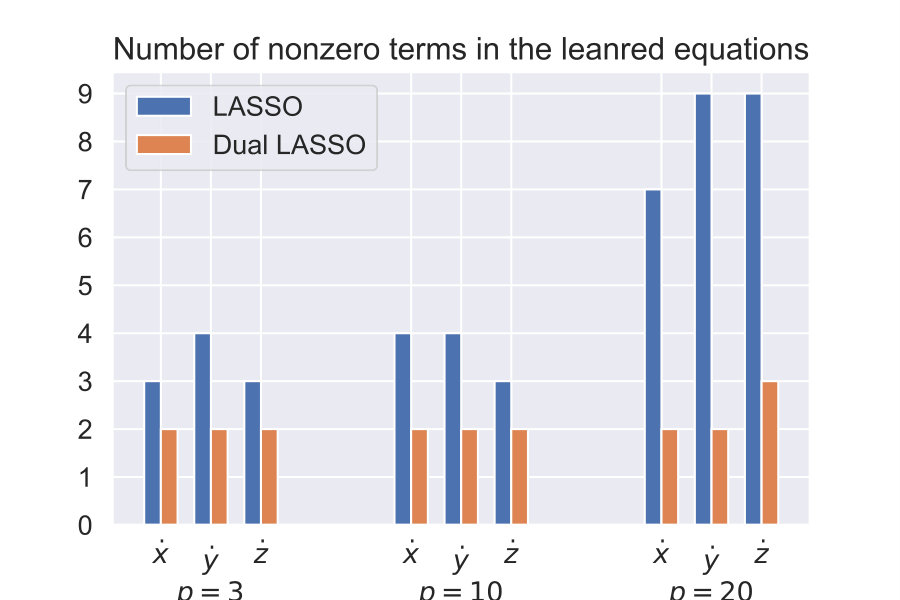 Figure 1
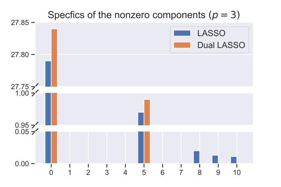 Figure 2
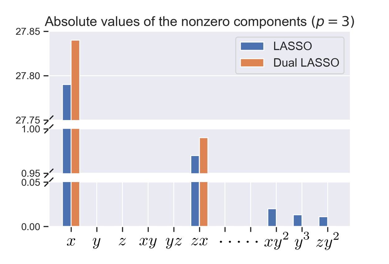 Figure 3
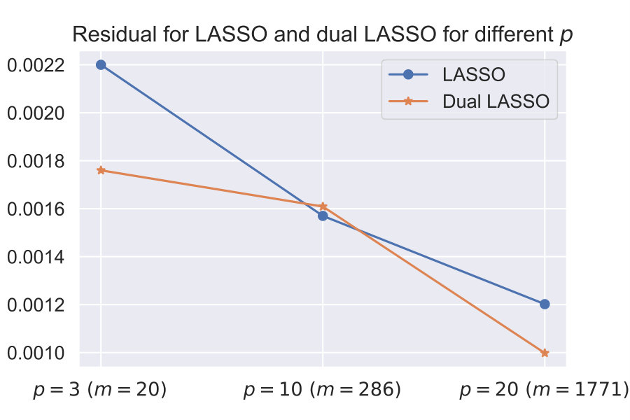 Figure 4
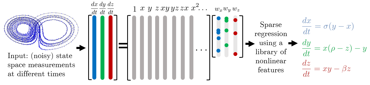 Figure 5
Peer Reviews
No public reviews on file for this paper yet. If you reviewed it on a platform where reviews are public (OpenReview, ICLR, NeurIPS, ICML), you can paste yours below so the community can read it here.
Videos
No videos yet. Explain this paper in a talk, walkthrough, or lecture? Add one.
Sparse Regression and Adaptive Feature Generation for the Discovery of Dynamical Systems
Chinmay S. Kulkarni [email protected]
Department of Mechanical Engineering, MIT
6.860: Statistical Learning Theory and Applications, Fall 2018, MIT
Abstract
We study the performance of sparse regression methods and propose new techniques to distill the governing equations of dynamical systems from data. We first look at the generic methodology of learning interpretable equation forms from data, proposed by Brunton et al. [3], followed by performance of LASSO for this purpose. We then propose a new algorithm that uses the dual of LASSO optimization for higher accuracy and stability. In the second part, we propose a novel algorithm that learns the candidate function library in a completely data-driven manner to distill the governing equations of the dynamical system. This is achieved via sequentially thresholded ridge regression (STRidge [17]) over a orthogonal polynomial space. The performance of the three discussed methods is illustrated by looking the Lorenz 63 system and the quadratic Lorenz system.
1 Introduction and Overview
The role of data today is no longer limited to the verification of first-principles-derived-models but it is also being used to learn such models. This is particularly important in non-autonomous nonlinear dynamical systems that describe a multitude of problems from science and engineering. Recent methods leverage the fact that most dynamical equations governing physical systems contain a few terms, making them sparse in high-dimensional nonlinear function space [3, 17]. By constructing an appropriate feature library based on the data coordinates, one can apply sparse regression to discover the governing equations of the dynamical system. Initial work in this field has mainly focused on the behavior of the approach with regards to noise, multi-fidelity data etc., however few have tried to improve upon the sparse regression algorithm at the core of the approach.
This is exactly the first focus area of the current work. We first look at the sparse regression method most commonly employed in this field: LASSO [18]. We point out the theoretical underpinnings of LASSO along with accuracy bounds. Although LASSO works well for uncorrelated features, for highly correlated it tends to choose a feature at random from each of the correlated groups [9]. When the feature library is built from data, higher order features are more correlated with each other, where LASSO potentially runs into difficulties. To alleviate these difficulties, we propose to solve the dual of LASSO to learn the governing equations. Even in the case of correlated features, the dual LASSO has a unique solution, which then allows us to correctly choose the present features. The second part of this work deals with the case when the exact function blocks that describe the dynamical system are not present in the feature library. We propose and investigate an approach to handle such cases by using an appropriate family of orthogonal functional basis to span the feature library. As the result may not be sparse in terms of the orthogonal functions, we resort to sequentially thresholded least squares (STRidge) algorithm [17] that does not impose sparsity, but chooses the dominant features.
These approaches are demonstrated on the Lorenz 63 system [15]and the quadratic Lorenz system [8]. We compare the performance of the LASSO and dual LASSO, and then use the approach of data-driven orthogonal regression to learn the feature library.
1.1 General Methodology
Let us assume that we have state space parameters (), with measurements for and at times (denoted by a superscript). If only state observations are available, the rate parameters can be computed using finite difference. This is followed by constructing a non-linear library of features using the state space parameters. The span of these features now describes the feature space. Typically we would construct this feature space through a class of functions that are dense in the space that our dynamical system lives in. In this work we assume a polynomial feature library. After constructing the feature library (say ), we formulate the regression problem as , where and are the unknown weights, with being the noise.
Often, dynamical models have a functional form where the terms live in a smaller manifold in the feature space. We thus use sparse regression to pick the relevant features. These features, with their corresponding coefficients describe the functional form of the governing equations. This procedure is pictorially illustrated in figure 1. For noisy observations, we carry out data filtering and smoothing at the input step and perform multiple sparse regression solves until convergence. However we do not focus on this, and we assume that we have noise free observations.
2 Sparse regression over fixed feature space
In this case, we assume that the feature library is fixed, and that we wish to find either the exact sparse equation form from this library or the closest approximation to the governing equation only from the terms in the library. The highest polynomial degree in the feature space () is . Then, the feature space contains terms of the form , such that . The number of solutions to this system (*i.e. *the number of terms in the feature library) is . Whereas, empirically the number of distinct terms in the governing equations is . Thus even for small enough , the terms in the feature library are much more in number than those to be chosen, which justifies sparse regression to select the features. Let us denote the coefficient matrix, obtained from the sparse regression solve by . The optimization problem with some form of penalty () is:
[TABLE]
To further select the features appropriately, we use our knowledge of the underlying physics of the dynamical system. Often, we have knowledge about the general scales of the state space parameters (for example, in the Lorenz system, the state space parameters represent the rate of convection, horizontal temperature variation and the vertical temperature variation). Thus, we know the the typical scales of these parameters from physics. Let us denote the scale of by , then . Thus, instead of selecting features based on their coefficient values, we select features by looking at their net magnitude, by replacing the state space parameters with their respective scales. We refer to this as ‘scale based thresholding’.
2.1 Sparsity through regularization (LASSO)
We now look at the use of LASSO for imposing sparsity. As is well-known, the LASSO penalty is , which serves as a convex counterpart to the non-convex norm. Kakade et al. [12] showed that the Rademacher averages for linear regressors with penalty are bounded by , where . We can then use the contraction property, assuming the Lipschitz constant of the LASSO problem to be (more details and methods to compute it may be found in [14, 13]) to obtain the bound of Rademacher averages of the loss function class . Using the symmetrization lemma, this yields a bound on the expected maximum error (uniform deviation), as given by Eq. (2).
[TABLE]
Note that even though we cannot explicitly compute the right hand side, we have , which renders this accuracy bound impractical. Thus, LASSO in the case of exceedingly high number of features does not provide good accuracy bounds. To alleviate this problem, we first use the SAFE bounds provided by Ghaoui et al. [10] to remove the irrelevant features and then apply LASSO over the remaining library. Even after weeding out the absent features, another important task that remains is to choose the hyperparameter . Literature widely suggests the order of to be [2], however choosing this parameter independent of the degree of correlation is not recommended [5]. It is further shown that the larger the correlation amongst the features, the smaller the value of [11]. Hebiri and Lederer [11] also prove that LASSO can achieve fast rate bounds (*i.e. *error bounded by ) even for correlated features. Even though reassuring, in practice this requires significant amount of tuning and cross validation, which is a major issue in the case at hand, as typically we only have sparse and limited observations of the physical states. Further, even though the LASSO fit is unique in case of high correlations, they are problematic for parameter estimation and feature selection [16, 19]. The pitfalls of LASSO (even after removing the irrelevant features using the SAFE rules) are that it requires significant hyperparameter tuning and it is extremely sensitive to for correlated features (observed empirically). These motivate us to instead formulate a new approach to solve the sparse regression problem.
2.2 Sparsity through dual LASSO regression
To overcome the difficulties in the application of LASSO (along with the SAFE rules), we formulate and solve its dual problem. In order for the LASSO solution (that is, the feature and parameter choices) to be unique, the feature matrix must satisfy the irrepresentability condition (IC) of Zhao and Yu [22] and beta-min condition of Bühlmann and Van De Geer [4]. The feature library violates the IC for highly correlated columns, leading to an unstable feature selection. However, even for highly correlated features, the corresponding dual LASSO solution is always unique [19]. The dual problem is given by Eq. (3) [16], which is strictly convex in (implying a unique solution).
[TABLE]
Now, let be a solution of Eq. (1) with LASSO penalty and be the unique solution to the corresponding dual problem Eq. (3). Then stationarity condition implies . Even though LASSO does not have a unique , the fitted value is unique, as the optimization problem Eq. (1) is strongly convex in for . We make use of this by first computing a solution to the primal LASSO problem and then computing the unique dual solution by using the primal fitted value and Eq. (3). Once we have the unique dual solution , we do feature selection by using the dual active set, which is same as the primal active set with high probability under the IC [9]. It is also be shown that features discarded by SAFE rules are the inactive constraints over the optimal dual solution [20], which justifies omitting them. KKT conditions imply:
[TABLE]
Eq. (4) gives us a direct way to compute the active dual set (which is the same as the active primal set with high probability) once we have . We discard the features for which and retain the others. This does not give us a good fit of the solution, so to compute the coefficients accurately, we perform ridge regression ( over these active features. This pseudocode for this is given in algorithm 1. We refer to this algorithm as ‘dual LASSO’.
3 Sparse Regression Over Adaptive Feature Space
In this section, we look at cases where the feature library is not known. If we have no prior belief over the form of the equations, we may not be able to construct an efficient feature library. In such situations, learning this library from data might be the most advantageous choice. One approach is to make the use of orthogonal functions of some parametric family, such as polynomials to construct this library. This ensures no correlation between the features and affords maximum freedom to the algorithm. The drawback in this case is that the regressor may not be sparse over this feature library.
3.1 Adaptive feature space growth through orthogonal regression
We propose the following approach for this purpose: Starting with an empty library, we recursively add a feature to it and compute the corresponding loss function of the resulting fit by using STRidge (Sec. 3.2). If the loss function decreases by more than a certain fraction, we keep this feature. Otherwise we discard it and look at the next orthogonal feature. Once every few of the addition timesteps, we perform a removal step. That is, we discard the feature(s) that do not result in a significant increase in the loss function (if any). This ensures that we do not keep lower order functions that may not be required to describe the equations as higher order functions are added. Our algorithm is inspired by previous greedy feature development algorithms by Efron et al. [7] (LARS), Zhang [21] (FoBa) etc. However these require pre-determined full possible feature space, whereas we construct new features on the fly. Once the equations are obtained in terms of these orthogonal polynomials, we distill their sparse forms by using symbolic equation simplification [1].
3.2 Sequentially thresholded ridge regression
To compute regressors over the orthogonal feature space, we use sequentially thresholded ridge regression (STRidge), proposed by Rudy et al. [17]. The idea is simple: we iteratively compute the ridge regression solution with decreasing penalty proportional to the condition number of , and discard the components using scale based thresholding (Sec. 2). As the feature matrix is orthonormal by construction, the analytical solution is . This algorithm is effective in choosing optimal features without necessitating sparsity. The overall pseudocode for learning the governing equations through adaptively growing the feature library is given by algorithm 2, and the corresponding results are presented in Sec. 4.
4 Results
For the first part (Sec. 2), our testbed will be the Lorenz 63 system (), given by Eq. (5).
[TABLE]
For the first part, we consider three polynomial feature libraries with and ( and ). The idea behind considering larger orders () is that it highlights the poor performance of LASSO for highly correlated features. Fig. (2a) shows the residual after the LASSO and the dual LASSO model fits. We can see that the residuals for both methods are comparable for all of the feature libraries, which empirically shows that the model fit even for a high degree of correlations is good for both the methods. Fig. (2b) plots the number of non-zero features in the equations for different values. LASSO has a much higher number of non-zero terms, and this number increases significantly with (and ), indicating instability of the solution. Dual LASSO performs very well, and the number of present features does not change for the most part with . Fig. (2c) plots the absolute weights for the components for the case for the equation. Dual LASSO retrieves the correct features (with accurate weights), while LASSO detects the correct features but also detects high order features that have low weights and are highly correlated to each other. This serves as a great validation of the superiority of dual LASSO over conventional LASSO for model discovery.
Now we look at the results for Sec. 3, on the quadratic Lorenz system (Eq. (6)) [8].
[TABLE]
We start with an empty feature library and and iteratively grow the feature space using algorithm 2 using Legendre polynomials (denoted by ), and removal step working every 10 addition steps (). The final obtained model is given in Eq. (7). We use symbolic simplification [1] to simply this model. Note that the model is not unique before symbolic simplification (as ). We also do scale based thresholding (Sec. 2) once after the symbolic simplification to remove any terms that may remain due to approximate factorization. The results before and after scale based thresholding are given in Eq. (8). We can see that this algorithm does a good job at identifying the correct governing equations by iteratively building the feature library, and does not include any incorrect features.
[TABLE]
[TABLE]
5 Conclusions and Future Work
In this work, we investigated LASSO, proposed dual LASSO and data driven feature learning approaches to solve the problem of discovering governing equations only from state parameter data. Future work directions involve extending the ideas of feature library building where one can construct the function to be added through a mix of a larger family of orthogonal functions. Approaches to involve kernel compositionality [6] to build these libraries can also be investigated.
The reference list from the paper itself. Each links out to its DOI / PubMed record.
- 1Bailey et al. [2014] David H Bailey, Jonathan M Borwein, and Alexander D Kaiser. Automated simplification of large symbolic expressions. Journal of Symbolic Computation , 60:120–136, 2014.
- 2Bickel et al. [2009] Peter J Bickel, Ya’acov Ritov, Alexandre B Tsybakov, et al. Simultaneous analysis of lasso and dantzig selector. The Annals of Statistics , 37(4):1705–1732, 2009.
- 3Brunton et al. [2016] Steven L Brunton, Joshua L Proctor, and J Nathan Kutz. Discovering governing equations from data by sparse identification of nonlinear dynamical systems. Proceedings of the National Academy of Sciences , 113(15):3932–3937, 2016.
- 4Bühlmann and Van De Geer [2011] Peter Bühlmann and Sara Van De Geer. Statistics for high-dimensional data: methods, theory and applications . Springer Science & Business Media, 2011.
- 5Dalalyan et al. [2017] Arnak S Dalalyan, Mohamed Hebiri, Johannes Lederer, et al. On the prediction performance of the lasso. Bernoulli , 23(1):552–581, 2017.
- 6Duvenaud et al. [2013] David Duvenaud, James Robert Lloyd, Roger Grosse, Joshua B Tenenbaum, and Zoubin Ghahramani. Structure discovery in nonparametric regression through compositional kernel search. ar Xiv preprint ar Xiv:1302.4922 , 2013.
- 7Efron et al. [2004] Bradley Efron, Trevor Hastie, Iain Johnstone, Robert Tibshirani, et al. Least angle regression. The Annals of statistics , 32(2):407–499, 2004.
- 8Eminağa et al. [2015] Buğçe Eminağa, Hatice Aktöre, and Mustafa Riza. A modified quadratic lorenz attractor. ar Xiv preprint ar Xiv:1508.06840 , 2015.