Prediction of galaxy halo masses in SDSS DR7 via a machine learning approach
Victor F. Calderon, Andreas A. Berlind

TL;DR
This paper introduces a machine learning method to predict galaxy halo masses more accurately than traditional techniques, using SDSS data and synthetic galaxy catalogues, with robust testing across different models.
Contribution
The study develops and validates a machine learning approach for galaxy halo mass prediction that outperforms existing methods and assesses its robustness across various simulation assumptions.
Findings
ML algorithms outperform HAM and DYN in mass prediction accuracy.
Training on synthetic data with different assumptions still yields better results than traditional methods.
The approach successfully applied to SDSS DR7 data to estimate galaxy halo masses.
Abstract
We present a machine learning (ML) approach for the prediction of galaxies' dark matter halo masses that achieves an improved performance over conventional methods. We train three ML algorithms (\texttt{XGBoost}, Random Forests, and neural network) to predict halo masses using a set of synthetic galaxy catalogues that are built by populating dark matter haloes in N-body simulations with galaxies, and that match both the clustering and the joint-distributions of properties of galaxies in the Sloan Digital Sky Survey (SDSS). We explore the correlation of different galaxy- and group-related properties with halo mass, and extract the set of nine features that contribute the most to the prediction of halo mass. We find that mass predictions from the ML algorithms are more accurate than those from halo abundance matching (\texttt{HAM}) or dynamical mass (\texttt{DYN}) estimates. Since the…
Click any figure to enlarge with its caption.
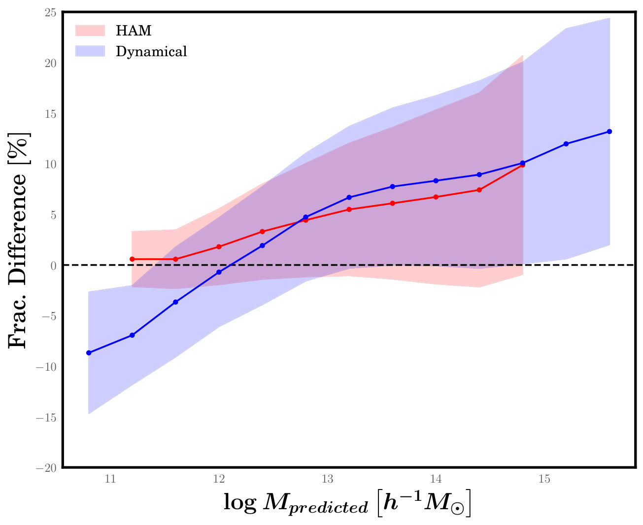 Figure 1
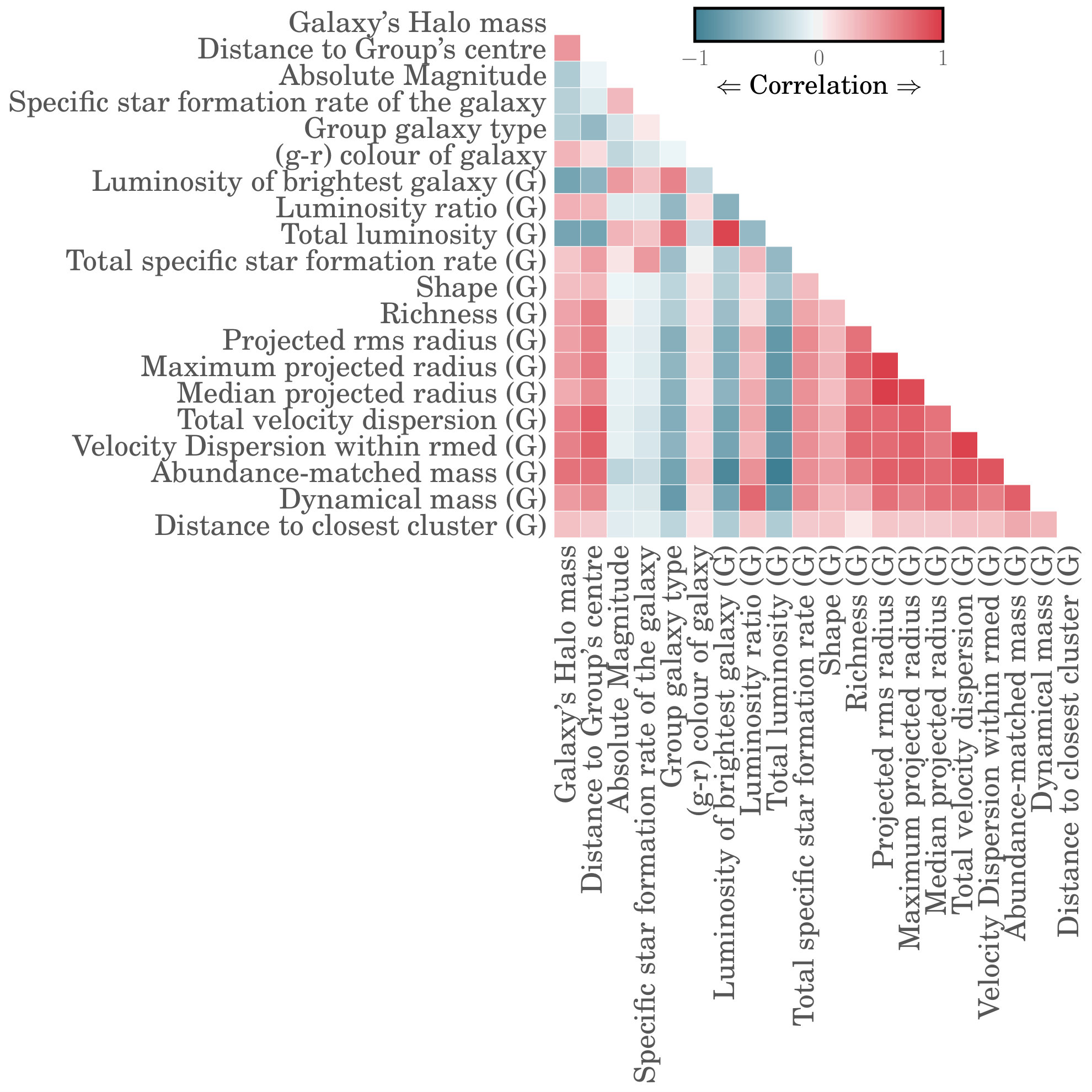 Figure 2
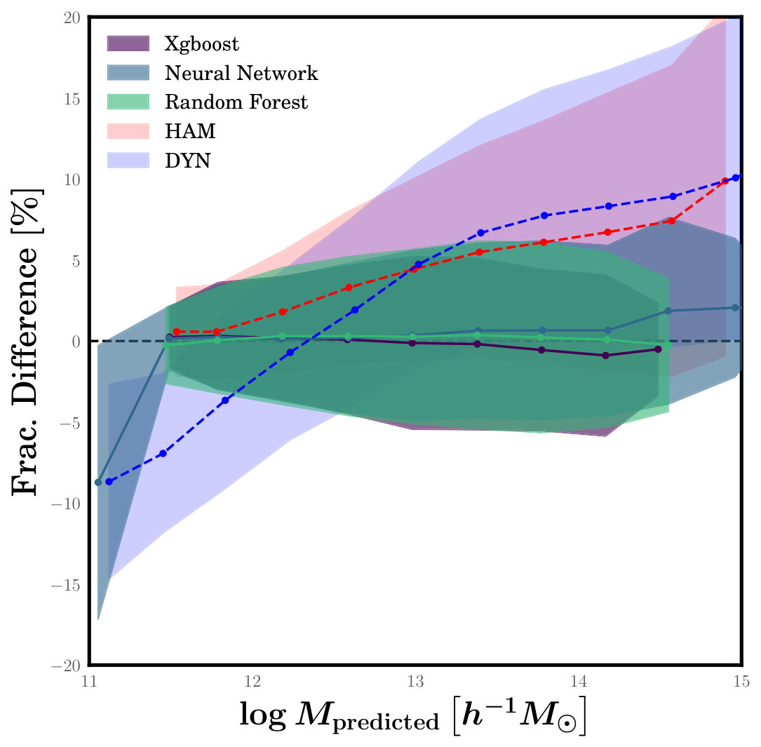 Figure 4
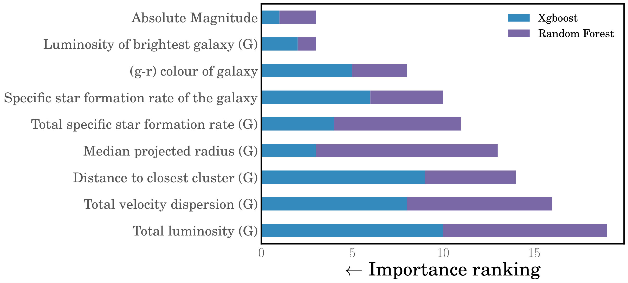 Figure 5
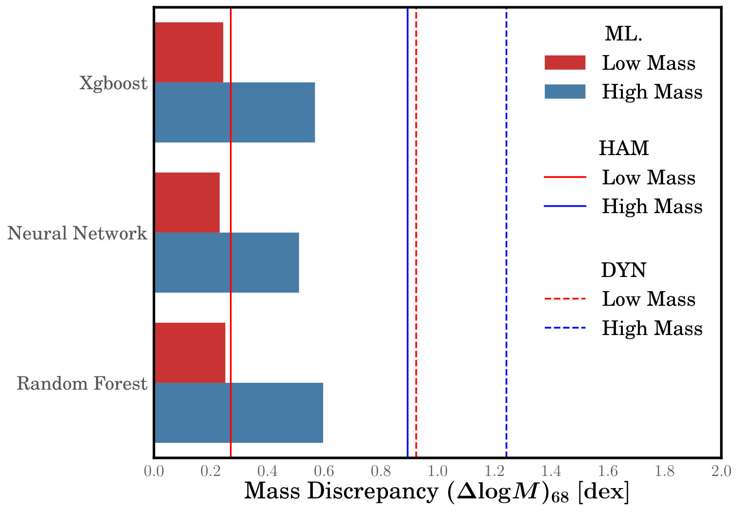 Figure 6
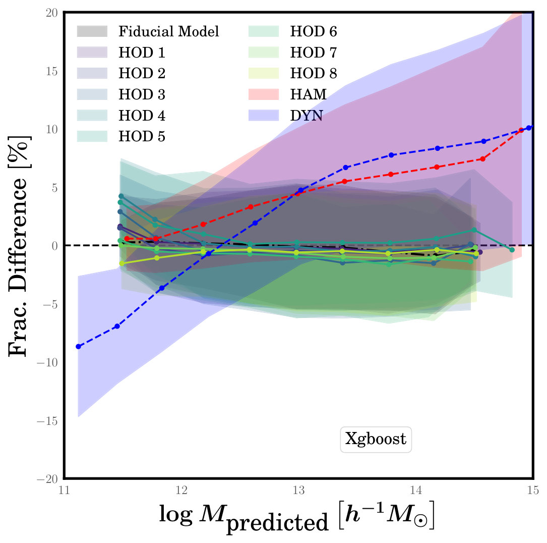 Figure 8
 Figure 10
 Figure 12
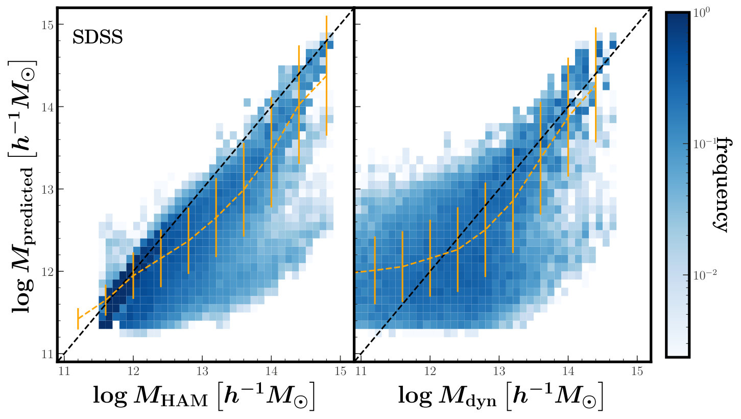 Figure 14
Peer Reviews
No public reviews on file for this paper yet. If you reviewed it on a platform where reviews are public (OpenReview, ICLR, NeurIPS, ICML), you can paste yours below so the community can read it here.
Videos
No videos yet. Explain this paper in a talk, walkthrough, or lecture? Add one.
\setremarkmarkupcolor=Changes@Color#1!20,size=color=Changes@Color#1!20,size=todo: color=Changes@Color#1!20,size=#1: #2
Prediction of Galaxy Halo Masses in SDSS DR7 via a Machine Learning Approach
Victor F. Calderon1, Andreas A. Berlind1
1 Department of Physics and Astronomy, Vanderbilt University, Nashville, TN 37235, USA Email: [email protected]
(Accepted XXX. Received YYY; in original form ZZZ)
Abstract
We present a machine learning (ML) approach for the prediction of galaxies’ dark matter halo masses that achieves an improved performance over conventional methods. We train three ML algorithms (XGBoost, Random Forests, and neural network) to predict halo masses using a set of synthetic galaxy catalogues that are built by populating dark matter haloes in N-body simulations with galaxies, and that match both the clustering and the joint-distributions of properties of galaxies in the Sloan Digital Sky Survey (SDSS). We explore the correlation of different galaxy- and group-related properties with halo mass, and extract the set of nine features that contribute the most to the prediction of halo mass. We find that mass predictions from the ML algorithms are more accurate than those from halo abundance matching (HAM) or dynamical mass (DYN) estimates. Since the danger of this approach is that our training data might not accurately represent the real Universe, we explore the effect of testing the model on synthetic catalogues built with different assumptions than the ones used in the training phase. We test a variety of models with different ways of populating dark matter haloes, such as adding velocity bias for satellite galaxies. We determine that, though training and testing on different data can lead to systematic errors in predicted masses, the ML approach still yields substantially better masses than either HAM or DYN. Finally, we apply the trained model to a galaxy and group catalogue from the SDSS DR7 and present the resulting halo masses.
keywords:
cosmology: observations — cosmology: large-scale structure of Universe – galaxies: groups — galaxies: clusters — methods: statistical
††pubyear: 2018 ††pagerange: Prediction of Galaxy Halo Masses in SDSS DR7 via a Machine Learning Approach– Prediction of Galaxy Halo Masses in SDSS DR7 via a Machine Learning Approach
1 Introduction
The practice of grouping galaxies observed in a galaxy catalogue into galaxy groups and clusters has been utilised extensively in astrophysics and cosmology, since the pioneering work of George Abell and Fritz Zwicky (Abell, 1958; Zwicky et al., 1968), who constructed cluster catalogues from the Palomar Observatory Sky Survey (POSS) using local galaxy surface number densities. Galaxy clusters represent the largest primordial density perturbations to have formed by now, and typically contain tens to hundreds of galaxies embedded within a common dark matter halo111Throughout this paper, we use the term ”halo” to refer to a gravitationally bound structure with overdensity , so an occupied halo may host a single luminous galaxy, a group of galaxies, or a cluster., thus tracing the high mass tail of the halo mass function. As a result, clusters constitute one of the most powerful cosmological probes and measurements of their abundance can be used to constrain cosmological parameters (e.g., Voit, 2005; Allen et al., 2011; Kravtsov & Borgani, 2012; Weinberg et al., 2013; Mantz et al., 2014). Additionally, our current understanding of galaxy formation and evolution revolves around the idea that all galaxies are formed and live within dark matter haloes. Therefore, galaxy groups and clusters, if identified correctly, can be used to study the galaxy-halo connection and thus how galaxies form and evolve within dark matter haloes. Whether we wish to use galaxy groups as probes of cosmology or galaxy formation, determining their masses accurately and robustly has proven to be a difficult task.
Galaxy groups and clusters can be identified in various ways. Originally, clusters were first detected as overdensities of galaxies in broad-band images in the visible spectrum (e.g. Abell, 1958; Zwicky et al., 1968). Since then, clusters have mainly been identified as overdensities of red galaxies in visible and IR bands (e.g. Gladders & Yee, 2005; Hao et al., 2010; Ascaso et al., 2012), as extended X-ray sources (e.g. Rosati et al., 2002; Vikhlinin et al., 2009), or by their signature in the cosmic microwave background (e.g. Marriage et al., 2011; Staniszewski et al., 2009; Ade et al., 2015). Since the early 1980’s and with the onset of redshift surveys, groups of galaxies have also been selected based on the closeness of galaxies in redshift space using three-dimensional algorithms. Many of these analyses have adopted the widely-used Friends-of-Friends percolation algorithm (Geller & Huchra, 1983) to place galaxies into groups and thus compile group catalogues. This algorithm links galaxies in pairs based on their separation along the line-of-sight or on the sky and places all linked galaxies into a single group. Numerous group galaxy catalogues have been constructed in this way for different redshift surveys, including the Center for Astrophysics Redshift Survey (CfA; Geller & Huchra, 1983), the Las Campanas Survey (Tucker et al., 1997), the Two Degree Field Galaxy Redshift Survey (2dFGRS; Merchán & Zandivarez, 2002; Eke et al., 2004; Yang et al., 2005; Tago et al., 2006; Einasto et al., 2007), the high-redshift DEEP2 survey (Gerke et al., 2005), the Two Micron All Sky Redshift Survey (Crook et al., 2007), and the Sloan Digital Sky Survey (e.g., Goto, 2005; Berlind et al., 2006).
Once galaxy groups and clusters are identified, mass measurements are needed to map observable properties to the underlying masses of dark matter haloes. Traditionally, there are two main methods to assign masses to galaxy groups and clusters that are built from galaxy redshift surveys, i.e., Halo Abundance Matching (hereafter HAM; e.g., Kravtsov et al., 2004; Tasitsiomi et al., 2004; Vale & Ostriker, 2004; Conroy et al., 2006) and dynamical mass estimates (hereafter DYN; e.g., Teague et al., 1990; Colless & Dunn, 1996; Fadda et al., 1996; Carlberg et al., 1997; Girardi et al., 1998; Brodwin et al., 2010; Rines et al., 2010; Sifón et al., 2013; Ruel et al., 2014). The HAM method assumes a monotonic relation between a theoretical mass-like quantity related to dark matter haloes and another observable quantity related to galaxies. This approach is simple yet powerful, wherein matching cumulative number densities of galaxies and haloes yields an implicit relationship between the theoretical quantity and the observational quantity (Hearin & Watson, 2013). HAM is typically used to connect galaxies to both host haloes and subhaloes, but in this context we refer to a variant of the method that connects galaxy groups to host haloes alone. For example, Yang et al. (2007) applied a halo-based group-finder (Yang et al., 2005) to the 2dFGRS and assigned halo masses to galaxy groups based on characteristic luminosity and characteristic stellar mass. Lim et al. (2017) extended this approach and applied a modified version of the same algorithm to multiple large redshift surveys. Calderon et al. (2018) applied the Berlind et al. (2006) algorithm to the SDSS and used HAM to estimate halo masses, based on the integrated luminosity of the groups. Moffett et al. (2015) did the same for the REsolved Spectroscopy of a Local VolumE (RESOLVE; Eckert et al., 2015) and the Environmental COntext catalog (ECO; Moffett et al., 2015). On the other hand, DYN estimates of clusters use the line-of-sight velocity dispersion of galaxies within clusters, together with measurements of their size, as dynamical tracers of the underlying gravitational potential. These estimates make use of variants of the virial theorem to estimate group masses.
Each of these approaches are not perfect, and may include possible biases or systematic errors in their mass estimates that may influence the final results. Old et al. (2014) performed an extensive comparison between various galaxy-based cluster mass estimation techniques that use position, velocities, and colours of galaxies to quantify the scatter, systematic biases and completeness of cluster masses derived from a diverse set of 25 galaxy-based methods. They found that abundance-matching and richness-based methods provide the best results, with some estimates being under- and overestimated by a factor greater than ten. Wojtak et al. (2018) studied these results further and found that contamination in cluster membership can affect the mass estimates greatly, with all methods either overestimating or underestimating the final cluster masses when applied to contaminated or incomplete galaxy samples, respectively. Additionally, Armitage et al. (2018) used the C-EAGLE galaxy clusters sample (Barnes et al., 2017) to quantify the bias and scatter of three mass estimators, and found no significant bias, but a large scatter when comparing estimated to true masses. For the case of HAM , Campbell et al. (2015) compared three different FoF-based group-finding algorithms by applying them to a realistic mock galaxy catalogue where the halo masses are known. They found that estimating group masses using HAM is limited by the intrinsic scatter in the relation between the observed quantity and the halo mass. They also show that errors in the group-finding process can cause catastrophic errors in estimated halo mass.
These previous works have demonstrated that galaxy groups and clusters identified in redshift surveys have mass estimates that are prone to large statistical and systematic errors, mostly due to failures of the group finding algorithms. These methods for estimating mass use one or two properties of groups, such as total luminosity in the case of HAM, or velocity dispersion and radius in the case of DYN. However, there are many additional properties of groups that should contain information about halo mass, such as colours and star formation rates, full density and velocity profiles, large scale environments, etc. This suggests the opportunity to apply nonparametric algorithms to analyse the abundant data at our disposal. There has been a significant increase in recent years in the number of studies applying machine learning (ML) techniques to astronomy. One of the most important applications of ML in astronomy is the classification of various objects, e.g. transient events (Mahabal et al., 2008) and galaxy morphology (Banerji et al., 2010). Other applications include the determination of photometric redshifts of galaxies from a set of broadband filters (Ball et al., 2007; Gerdes et al., 2010), the assignment of dark matter haloes to generate synthetic catalogues from N-body simulations (Xu et al., 2013; Kamdar et al., 2016a, b) and the study of the structure of the Milky Way (Riccio et al., 2016). Relevant to this work, ML has also been used to improve galaxy cluster dynamical mass measurements by employing the entire line-of-sight velocity PDF information of galaxy clusters (Ntampaka et al., 2015, 2016). More recently, ML algorithms have been used to measure cluster masses using a combination of dynamical and X-ray data (Armitage et al., 2019), and more complex algorithms have been employed to estimate the masses of galaxy clusters using synthetic X-ray images from cosmological simulations (Ntampaka et al., 2018). However, these studies were restricted to the massive cluster regime.
In this paper, we explore the possibility of employing ML techniques to estimate the halo masses of galaxies in a wide range of mass. We adopt observed properties of both the galaxies and their groups to act as features and we train the ML algorithms on synthetic data. This paper is organised as follows. In 2, we describe the observational and simulated data used in this work (2.1), introduce the set of features used in this analysis (2.2), and present the main set of ML algorithms that we use (2.3). In 3, we provide the main analysis of feature selection (3.1), and present our main results of mass estimates (3.2). In 4 we also present a detailed examination of how mass estimates may vary depending on the choice of HOD parameters (4.1), velocity bias, (4.2), or scatter in the mass-to-light ratio of central galaxies (4.3). In 5, we apply our trained algorithms to SDSS, and present the resulting galaxy catalogue with various estimates of halo mass. We summarise our results and discuss their implications in 6. The Python code and catalogues used in this project will be made publicly available on Github222https://github.com/vcalderon2009/SDSS_Groups_ML upon publication of this paper.
2 Data and Methods
In this section, we present the datasets used throughout this analysis, and introduce the main ML algorithms and statistical methods that we use to estimate the halo masses of galaxies. In 2.1, we briefly describe the SDSS galaxy sample and synthetic galaxy catalogues that we use, along with the parameters that are included in these catalogues. In 2.2, we introduce the different features that we use for training our ML predictors, and provide a guide on how these are calculated. Finally, in 2.3 we provide a brief overview of the different algorithms that we use in this analysis, as well as the default tuning parameters used by each algorithm.
2.1 SDSS Galaxy Sample and Mock Galaxy Catalogues
For this analysis, we make use of a modified version of the galaxy and group galaxy catalogues used in Calderon et al. (2018). We will provide a brief description of the galaxy sample used, and also an overview of the synthetic galaxy and group galaxy catalogues used in this analysis.
2.1.1 SDSS Galaxy Sample
For this analysis, we use data from the Sloan Digital Sky Survey (hereafter SDSS; York, 2000). SDSS collected its data with a dedicated 2.5-meter telescope (Gunn et al., 2006), camera (Gunn et al., 1998), filters (Doi et al., 2010), and spectrograph (Smee et al., 2013). We construct our galaxy sample from the large-scale structure sample of the NYU Value-Added Galaxy Catalogue (NYU-VAGC; Blanton et al., 2005), based on the spectroscopic sample in Data Release 7 (SDSS DR7; Abazajian et al., 2009). The main spectroscopic galaxy sample is approximately complete down to an apparent r-band Petrosian magnitude limit of . However, we have cut our sample back to so it is complete down to that magnitude limit across the sky. Galaxy absolute magnitudes are k-corrected (Blanton et al., 2003) to rest-frame magnitudes at redshift .
We construct a volume a volume-limited galaxy sample that contains all galaxies more luminous than , and we refer to this sample as Mr19-SDSS. The redshift limits of the sample are and and it contains 90,893 galaxies with a number density of . The sample includes the right ascension, declination, redshift, and colour for each galaxy.
To each galaxy, we assign a star formation rate (SFR) using the MPA-JHU Value-Added Catalogue DR7333https://wwwmpa.mpa-garching.mpg.de/SDSS/DR7/. This catalogue includes, among many other parameters, stellar masses based on fits to the photometry using Kauffmann et al. (2003) and Salim et al. (2007), and star formation rates based on Brinchmann et al. (2004). We cross-match the galaxies of the NYU-VAGC to those in the MPA-JHU catalogue using their MJD, plate ID, and fibre ID. A total of 5.65% of galaxies in the sample did not have corresponding values of SFR and were removed from the main sample. This leaves a sample of 85,578 galaxies. For each of these galaxies, we divide its SFR by its stellar mass to get specific star formation rates, sSFR.
Ultimately, we identify galaxy groups using the Berlind et al. (2006) group-finding algorithm. This is a Friends-of-Friends (FoF; Huchra & Geller, 1982) algorithm that links galaxies recursively to other galaxies that are within a cylindrical linking volume. The projected and line-of-sight linking lengths are and in units of the mean inter-galaxy separation, respectively. This choice of linking lengths was optimised by Berlind et al. (2006) to identify galaxy systems that live within the same dark matter halo. In each group, we define the most luminous galaxy (in the r-band) to be the ’central’ galaxy. The rest of the galaxies are defined as ’satellite’ galaxies.
In previous works, we have estimated the total masses of the groups via abundance matching, using total group luminosity as a proxy for mass. Specifically, we assume that the total group r-band luminosity increases monotonically with halo mass , and we assign masses to groups by matching the cumulative space densities of groups and haloes:
[TABLE]
To calculate the space densities of haloes, we adopt the Warren et al. (2006) halo mass function assuming a cosmological model with , , (100 ) = 0.7, , and . We refer to these abundance matched masses as group masses, . In this paper, we also use a dynamical mass estimate for each group, as well as other group properties, which are described in § 2.2.
2.1.2 Mock Galaxy Catalogues
In order to make proper predictions of the halo masses of galaxies, we need a training dataset where the halo mass of each galaxy is known. This necessitates that we use mock, rather than real data. However, the accuracy of our predictions hinges on the degree to which the mock data are truly representative of the observable Universe. Therefore, the mock dataset must not only contain the same observable properties that we will use as features in the SDSS data, it should also faithfully reproduce the true correlations between these properties and halo mass. At a minimum, the training data should be able to accurately reproduce the observed clustering of galaxies and the joint distributions of "observed" galaxy properties.
For this project, we use a suite of 10 realistic synthetic galaxy and group galaxy catalogues similar to Calderon et al. (2018), with the one exception that we use a different definition when identifying dark matter haloes, i.e. we use a spherical-overdensity (SO) definition as opposed to the Friends-of-Friends (FoF) halo definition used in Calderon et al. (2018). These synthetic catalogues are based on the Large Suite of Dark Matter Simulation (LasDamas) project444http://lss.phy.vanderbilt.edu/lasdamas/ (McBride et al., 2009), and have the same clustering and same distributions of "observed" properties as the SDSS data (luminosity, colour, sSFR, and Sérsic index). We use an Halo Occupation Distribution (HOD; Berlind & Weinberg, 2002) model to populate the DM haloes with central and satellite galaxies, whose numbers as a function of halo mass were chosen to reproduce the number density, , projected 2-point correlation function, , and group multiplicity function, , of the Mr19-SDSS sample. Specifically, we use the best-fit HOD values of Sinha et al. (2018) for the case of the Mr19-SDSS sample, the ‘LasDamas’ cosmology, the ‘Mvir’ halo definition, and the ‘PCA’ option.
Once galaxies are placed in haloes, we assign luminosities and colours using modified versions of the Conditional Luminosity Function (CLF; Yang et al., 2003) framework and the Zu & Mandelbaum (2016) halo-quenching model. This approach yields luminosity and colour distributions as well as luminosity- and colour-dependent clustering that are in agreement with SDSS measurements. The resulting mock catalogues have been analysed in exactly the same way as the SDSS data (i.e. same group-finding algorithm, same method of assigning group masses, etc). In their final version, the catalogues contain information on various galaxy-related properties (e.g., sSFR, Sérsic index, colour, luminosity) and group-related properties (e.g., group richness, groups’ total r-band absolute magnitudes, velocity dispersion within the groups, etc).
For a more detailed explanation of what went into producing the set of mock catalogues used in this analysis, we refer the reader to §2.3 of Calderon et al. (2018).
2.2 Galaxy properties as features
As part of our analysis, we must make a decision on which features to use when training the ML algorithms to predict the masses of galaxies’ dark matter halos. The set of features that we use includes properties of the galaxy in question as well as properties of the group to which the galaxy belongs. All features can be observed and measured in the SDSS. Here we provide a list of the features that we consider initially with a description of how each is computed. Later on we reduce this to a shorter list using a feature selection algorithm.
Galaxy-related features
- 1
Distance to group’s centre: This feature refers to how far a galaxy is from the centre of its corresponding galaxy group. This variable is given in units of of , but it is calculated in three-dimensional space so it is dominated by the velocity component of the galaxy’s position. The centre of the group is computed as the centroid of the group’s member galaxy positions. 2. 2
Absolute Magnitude: r-band absolute magnitude of the galaxy, k-corrected to . 3. 3
Specific star formation rate of the galaxy, sSFR: Logarithmic value of the specific star formation rate of the galaxy. As mentioned in 2.1.2 and in Calderon et al. (2018), in our mock catalogues these sSFRvalues were assigned using the Zu & Mandelbaum (2016) halo-quenching model, and matched to the distribution of sSFR values in SDSS DR7 through abundance matching. 4. 4
Group galaxy type: The galaxy type of the galaxy, in terms of its galaxy group. We denote a value of "1" if the galaxy is a group central, and a "0" if the galaxy is a group satellite. After determining the group membership of each galaxy, we designate the brightest galaxy of the group in the r-band as the group central, while the rest of galaxies are identified as group satellites. Hence, a galaxy group is composed of one bright group central and a number of group satellites. This criterion is motivated by the idea that central galaxies grow in mass and brightness by galactic cannibalism (Dubinski, 1998; Cooray & Milosavljević, 2005), while satellite galaxies experience a series of events that strip them from their mass and inhibit star formation (e.g. ram-pressure stripping and tidal stripping). 5. 5
** colour of galaxy**: The difference between the absolute magnitudes in the g-band and r-band, after these have been k-corrected to . In our mock catalogues, galaxy colours were assigned in a manner similar to that of sSFR.
Group-related features
- 6
Luminosity of brightest galaxy: r-band absolute magnitude value of the brightest galaxy in the group that the galaxy in question belongs to. This absolute magnitude is the same as that of the group central galaxy, according to our designation of group centrals and group satellites. 2. 7
Luminosity ratio: Ratio between the r-band luminosity of the brightest and second brightest galaxies in the group. 3. 8
Total luminosity, : The total r-band luminosity of the group is the sum of the r-band luminosities of its member galaxies. We compute the total group r-band absolute magnitudes as
[TABLE]
where ‘‘ corresponds to the number of member galaxies in the group, and ‘‘ to the k-corrected r-band absolute magnitude of the i-th galaxy in the galaxy group. The resulting variable is the groups’ total r-band absolute magnitude, . 4. 9
Total specific star formation rate, : Logarithmic value of the total specific star formation rate of the group. For each group, the total specific star formation rate is calculated as:
[TABLE]
where ‘‘ refers to the number of member galaxies in the galaxy group, ‘‘ and ‘‘ to the stellar mass and star formation rate of the i-th galaxy in the galaxy group. 5. 10
Shape: The shape of the group is calculated by first computing the eigenvalues of the group’s moment of inertia tensor, and then by taking the ratio between the values of the largest and second largest eigenvalues. This ratio is what we designate as the group shape feature. 6. 11
Richness: Richness is the total number of galaxies in the galaxy group. A galaxy group can be composed of a single galaxy, or many galaxies. 7. 12
Projected rms radius, : Projected rms radius of the group. It is given by
[TABLE]
where is the projected distance between each member galaxy and the group centroid. This variable is only computed for galaxy groups with two or more member galaxies. For groups with just one member galaxy, we assign a value of ’0’ to . 8. 13
Maximum projected radius, : The total radius of the galaxy group corresponds to the projected distance between the centre of the galaxy group and and the most distant member galaxy of the group. 9. 14
Median projected radius, : The median radius of the galaxy group is the median distance between the centre of the group and the group’s member galaxies. 10. 15
Total velocity Dispersion, : We compute a group one-dimensional velocity dispersion given by
[TABLE]
where is the total number of galaxies in the group, is the mean velocity of the group, and is the velocity of each member galaxy. This variable is only computed for galaxy groups with two or more member galaxies. For groups with just one member galaxy, we assign a value of ’0’ to . 11. 16
Velocity dispersion within : Similar to . We compute a one-dimensional velocity dispersion of the galaxies that are within with Equation 5, but only using galaxies within the designated radius from the centre of the galaxy group. 12. 17
Abundance-matched mass, : We estimate the total mass of the group via abundance matching. This method assumes a monotonically increasing relationship between the group total luminosity, , and the dark matter halo mass. We adopt the Warren et al. (2006) mass function for this purpose. 13. 18
Dynamical mass: We follow the prescription from Girardi et al. (1998) for estimating the group dynamical mass, using and as follows
[TABLE]
where is the gravitational constant. A is a fudge factor that we use to remove any systematic offset between the dynamical mass estimate and the true halo mass in the cluster mass regime. Based on tests with our mock catalogs, we set this fudge factor to a value of ‘1.04’. With this value of A, the above equation recovers the correct halo mass for a massive halo in the ideal case where the radius and velocity dispersion of the halo are known perfectly. 14. 19
Distance to closest cluster: Distance to the closest cluster of galaxies that is at least a factor of 10 times more massive than the host group of the galaxy in question. Masses are measured using halo abundance matching and the distance is in units of and is calculated in three-dimensional space. If no such cluster of galaxies is to be found, we assign a value of ’0’ to this variable.
This list of features contains spectro-photometric properties of the galaxies, sizes and velocity dispersions of their groups, two halo mass estimates (one derived from spectro-photometric properties, i.e., HAM , and one derived from group size and velocity dispersion, i.e., DYN ), a group morphological parameter, and a large-scale environmental metric. All of these features are expected to contain information about halo mass.
2.3 Machine Learning algorithms
Machine learning is an inventive field in computer science, with a variety of different applications in a number of areas. As mentioned in 1, ML algorithms are able to learn non-parametric relationships between some input data and an expected output, without having to explicitly provide an analytic prescription. In the case of supervised learning, which is the type of ML used in this paper, a training dataset is provided, and the ML algorithms try to learn the mapping between the set of features, , and the expected output, . Once the algorithm is trained, it is tested on a different ‘test’ dataset in order to quantify how well it works. Ultimately, the goal is to apply the algorithm to an application dataset where is not known.
For our study, we test the performance of 3 different flavours of ML algorithms in order to see which algorithm can provide us with the best prediction for the halo masses of galaxies. We use the Random Forest an Neural Network algorithms from the python package scikit-learn555http://scikit-learn.org/ (Pedregosa et al., 2012), as well as the XGBoost algorithm 666https://xgboost.readthedocs.io/.
2.3.1 Random Forest
One of the ML algorithms that we use in this analysis is Random Forests (hereafter RF; Breiman, 2001). A random forest is an ensemble learning technique that builds upon a collection of tree-structured classifiers, also known as decision trees. For the purpose of this analysis, we implement RF for regression rather than for classification, and decision trees are to be referred as regression trees in this context. RF makes use of the bagging method, in which it generates n samples from the dataset, trains each sample individually and averages all of the predictions at the end. For a more comprehensive account of this technique, the reader is referred to Breiman et al. (1984). We implement the scikit-learn version of RF, RandomForestRegressor, with its default settings.
2.3.2 XGBoost
XGBoost (Chen et al., 2006) is part of the family of boosting algorithms, which makes use of the boosting method. In Boosting, unlike in Bagging, the algorithm generates random samples for training with replacement over weighted data. Each of these regression trees are referred to as weak learners, and they each get assigned weights based on the accuracy of their predictions. After these weak learners are trained, the weighted averages of each of their estimates are used to compute the final predictions. The combination of weak learners is referred to as strong learners. For a more in-depth discussion of XGBoost and its different features, the reader is referred to the online documentation 6.
2.3.3 Neural network
The last ML algorithm used in this analysis is the simplest type of a neural network (NN), i.e. the Multi-Layer Perceptron (MLP). A MLP is a model with interconnected information processing units, often referred to as neurons, that learns the mapping given a training set , with being the input features and the target elements to predict. We implement the scikit-learn version of a 3-layer MLP with each layer containing 100 neurons. We refer the user to the scikit-learn documentation5 for a more comprehensive account of this method.
3 Training and Testing ML algorithms
In this section, we present results from the training and testing of the three ML algorithms for predicting the halo masses of galaxies in SDSS DR7. Moreover, we compare these predictions to the more traditional estimates from halo abundance matching (HAM) and dynamical mass measurements (DYN). In 3.1, we present the set of features that contribute the most to the overall prediction of halo mass in order to reduce the dimensionality of our feature space in further training. In 3.2, we present results from the training and testing phases of each of the three ML algorithms using our synthetic catalogues of the Universe. The mock catalogues used in the training and testing phases are built using the same HOD model and thus represent the overly optimistic scenario in which the training data perfectly represents the real universe. Results in this section thus serve as a proof of concept that ML is a feasible method of determining the halo masses of galaxies. We explore the more realistic case that the training data is drawn from a different underlying model than the real universe in 4.
3.1 Feature Selection
In § 2.2 we presented a list of 19 properties of galaxies and their groups that may contain useful information about halo mass. In this section we analyse the predictive power of these features in order to eliminate ones that are not as useful and thus reduce the overall number of features that we will use as inputs to the ML algorithms. This is conventionally referred to as feature selection, and it plays an important role into the training process of a ML algorithm. Reducing the dimensionality of the feature space is desirable because it reduces the computational cost of ML algorithms and can also improve their predictive performance.
Before we determine the importance of each feature for the prediction of halo mass, we first explore the amount of correlation among the different features from 2.2. Figure 1 presents the correlation matrix of these 19 features as measured from our mock galaxy catalogues. The matrix shows the correlation coefficient between each pair of features, with red and blue shadings corresponding to positive or negative correlation, respectively. The matrix also includes halo mass in the first column and thus reveals how much each feature is correlated with the quantity we are trying to predict. Figure 1 shows that almost all 19 of our features exhibit correlations with halo mass. Additionally, many of the features are highly correlated with each other, as expected, and are thus unlikely to contain independent information about halo mass.
To quantify the importance of each feature for the purpose of feature selection, we use the native feature importance calculation within the RF and XGBoost algorithms (the NN algorithm does not compute such a statistic). In general, these algorithms estimate the importance of a feature by calculating how much it is used to make key decisions with their decision trees. Each feature gets an importance score allowing us to compare them to each other and rank them. Though later on we will split our 10 mock catalogues into training and testing subsets, for the purpose of feature selection we use them all to train the RF and XGBoost algorithms. Each algorithm then produces a ranked list of the 19 features in order of their importance, as discussed above. Though the two algorithms differ in their detailed ranking of features, they are generally consistent and are almost in perfect agreement on which features land in the top nine (out of 19). The remaining set of features do not contribute much to the overall prediction of halo mass and so we focus on these nine features moving forward.
Figure 2 shows the feature importance ranks for these top nine features for both the XGBoost and RF algorithms. In the case of each feature, the length of the blue and purple bar indicates its importance rank as calculated by XGBoost and RF , respectively, with shorter bars corresponding to more important features. We estimate the overall importance of each feature by adding its two ranks (the combined length of the blue and purple bars) and we order the features in Figure 2 according to this overall score. The figure shows that the luminosity of the galaxy itself and the luminosity of the brightest galaxy in the galaxy’s group are the overall most useful features in predicting halo mass, while the total group luminosity is the least useful from this set of top nine features.
We select these top nine features that contribute the most to the prediction of halo mass as our final set of features moving forward.
Final set of features
- 1
Galaxy’s r-band absolute magnitude 2. 2
Luminosity of the brightest galaxy in the group 3. 3
Galaxy’s colour 4. 4
Galaxy’s specific star formation rate 5. 5
Group’s total specific star formation rate 6. 6
Group’s median projected radius 7. 7
Distance to the closest cluster 8. 8
Group’s total velocity dispersion 9. 9
Group’s total r-band absolute magnitude
For the rest of the analysis in this paper, we will exclusively use this set of features to train the various ML algorithms and evaluate their performance at correctly predicting halo masses.
3.2 Training and Testing
Now that we have a final list of nine input features, we can proceed to the training and testing of the ML algorithms. We start with our set of 10 mock galaxy catalogues, each of which has the same volume and approximate number density as the Mr19-SDSS sample. Combined, these catalogues contain a total of 758,528 mock galaxies. For each galaxy we have values for the nine input features as well as the target halo mass. We also have the traditional HAM and DYN mass measurements to compare against.
We split the mock data into training and testing sets. The training set consists of 8 of the 10 catalogues, while the testing set consists of the remaining 2. We will use the testing set to evaluate how well the trained algorithms perform. It is important to perform this evaluation on an independent set of data from the training set in order to guard against the problem of over-fitting. Sometimes ML analyses also use a third, validation, dataset for the purpose of tuning the hyper-parameters of a given ML algorithm. However, in this paper we choose to adopt the default values of hyper-parameters and thus we do not need to add a validation step to our workflow.
After training the three ML algorithms to predict the dark matter halo masses of mock galaxies in the training set, we apply these trained algorithms to the testing data and get a list of predicted masses, , for these galaxies. We then compare these predictions against the true halo masses, , and compute the fractional difference between their logarithmic values as
[TABLE]
Each galaxy in the testing set gets three values of (one for each ML algorithm), which are essentially the fractional errors in the ML predictions. Note that these are errors in the logarithm of halo mass. A value of 5% thus corresponds to a fractional error in mass of % for the mass range we consider here. For comparison, we also calculate using the HAM and DYN masses in place of . This will allow us to examine how well the ML algorithms perform relative to traditional methods for estimating halo mass.
Figure 3 presents results for , as a function of predicted mass, for different methods of estimating the halo masses of galaxies. The solid, coloured lines correspond to the mean fractional difference of galaxies in bins of , while the shaded regions represent the ranges of . We show predictions made by the XGBoost, RF, and NN algorithms, and compare these to the mass estimates obtained from HAM and DYN. Figure 3 shows promising results, in that all three ML algorithms are performing significantly better at predicting the mass of a galaxy’s host halo than either HAM and DYN. Specifically, HAM yields halo masses that are unbiased on average at low masses and have a error of , but it systematically overestimates masses on average at high masses, reaching a systematic error as high as in the cluster regime. Moreover, the scatter grows to in this regime as well. DYN exhibits even worse performance since it has similar poor performance for large masses, but also does badly at low masses, systematically underestimating masses on average as much as . In contrast, the three ML algorithms yield predicted masses that are unbiased on average at all masses and have a scatter in of .
To understand the poor performance of the HAM and DYN methods, it is important to consider that we are not evaluating the ability of these methods to correctly estimate the halo masses of galaxy groups, but rather of individual galaxies. Grouping errors made by the group-finding algorithm can thus cause catastrophic errors in the halo masses of galaxies that have been incorrectly grouped. For example, if the group-finder incorrectly merges together a few galaxies that live in small haloes with the galaxies of a large halo to yield a single massive galaxy group, both HAM and DYN will estimate a large halo mass for this group and, thus, for all its members. The error in this estimate will be small for the galaxies that actually belong to the large halo, but will be enormous for the galaxies that were mistakenly grouped. It is these catastrophic errors that drive both methods to overestimate the masses of galaxies on average in the high mass regime in Figure 3. At low masses, where most galaxies live in groups, HAM does a good job at recovering the mass because galaxy luminosity correlates strongly with mass. DYN, however, does poorly because dynamical measurements are very unreliable for systems with a small number of galaxies. The ML algorithms have the advantage that they use additional information that can help fix some of the problems caused by grouping errors. In the example above, the colours of incorrectly grouped galaxies are likely different from those of actual satellite galaxies in massive halos and the ML algorithms exploit this to distinguish between the two. An exciting possibility that arises from this is that the halo masses predicted by ML could be used to improve the group-finding itself since galaxies whose predicted masses are much smaller than the groups they’ve been assigned to could be removed from them. We return to this point in the final section.
Another way to quantify the effectiveness of these algorithms at predicting halo masses is to determine the percentile discrepancy between the true and predicted halo masses across a big range of masses. To compute this statistic, we first determine the absolute value of the log-difference between predicted and true halo mass, and rank-order them from smallest to largest. We then determine the discrepancy that corresponds to the 68% of galaxies that are best predicted. This statistic is given by the following equation:
[TABLE]
In other words, 68% of galaxies have their masses predicted with an error less than . We split the test sample into a low-mass and high-mass galaxy sample. Galaxies with are assigned to the low-mass sample, while those with are assigned to the high-mass sample. For each sample, we compute for each ML algorithm, and compare them to those for HAM and DYN. This statistic shows how well each method is at estimating the halo masses in these two mass regimes.
Figure 4 presents the results for the typical mass error . Horizontal bars show values for the three ML algorithms, while solid and dashed vertical lines show results for the HAM and DYN methods, respectively, for comparison. In all cases, results for galaxies with low predicted masses are shown in red, while results for galaxies with high predicted masses are shown in blue. Figure 4 shows clearly that the three ML algorithms exhibit similar performance and they significantly outperform traditional methods in most cases. HAM does well at low masses, but at high masses its error is larger than ML methods. DYN does poorly in both mass regimes, with a typical error that is times larger than that for ML methods. More specifically, HAM is able to estimate halo masses to within a dex and dex for the low-mass and high-mass regimes, respectively. On the other hand, DYN can only recover halo masses to within dex and dex for the low-mass and high-mass regimes, respectively. The corresponding errors for the XGBoost, RF, and NN ML algorithms range from, dex and dex for the low-mass and high-mass samples, respectively.
In summary, we find that we are able to obtain better mass estimates for a galaxy’s host halo by using ML methods in place of the more traditional mass estimators, such as HAM or DYN . This statement is true regardless of predicted mass, . However, so far this statement only holds for the case in which the training and testing samples share the same underlying model that connects galaxies to dark matter halos. This is not likely to be true when we apply the trained models to real SDSS data. We address this issue in the next section.
4 Are Mock-Trained Models Universally Applicable?
The results shown in 3.2 support the notion that we can obtain better halo mass estimates for galaxies by employing ML algorithms instead of the traditional HAM or DYN methods. We evaluated the performance of the ML algorithms using a testing set of mock galaxy catalogues that are independent from the set that we used to train the models. In this context, “independent” means that they are constructed from cosmological N-body simulations that are independent realisations of the density field (i.e., have initial conditions with different random phases). However, the testing catalogues adopt the same prescription for populating dark matter halos with galaxies and assigning them observed properties like luminosity and colour. A better approach would be to test the ML algorithms using catalogues that were built with different such prescriptions, since the real universe is unlikely to perfectly conform to the assumptions made in the training phase. In this section, we test the impact of these assumptions in order to assess whether mock-trained models can be applied to the real universe.
4.1 Varying HOD models
The first step we make to build mock galaxy catalogues from a dark matter halo distribution is to populate the halos using a HOD model. This model specifies the number of central and satellite galaxies that are placed in each halo. The model is flexible and has five free parameters. We use the best-fit parameter values of Sinha et al. (2018), which ensure that the number density, clustering, and group statistics of our catalogues match those observed in the SDSS. This is the fiducial HOD model that we used to train and test our models in § 3. To test how sensitive our results are to the HOD model of the testing sets, we now produce different versions of our two synthetic testing catalogues, each with different values for the five HOD parameters. We select the parameter sets from the Sinha et al. (2018) MCMC chain so that the resulting mock catalogues are still consistent with SDSS observations. We then run the previously trained ML algorithms on these new test mock catalogues to investigate how much performance we lose from modifying the HOD model in the testing phase.
Figure 5 shows the fractional difference between predicted and true halo mass, , for these new test sets. The figure is similar to Figure 3, except that it only shows results for the XGBoost algorithm and it focuses on the different HOD models instead. Also shown are the HAM and DYN results for comparison, which are applied to the fiducial test catalogues. We have also done the same tests using the RF algorithm and obtained similar results. Figure 5 reveals that the performance of the ML algorithm degrades significantly at low masses when it is applied to testing catalogues with different HOD models. For predicted masses larger than the effect is negligible and ML clearly outperforms the HAM and DYN methods just as it did when tested on the fiducial model. However, for , the mean is significantly biased for some of the HOD models, reaching values as high as 4%.
To understand why the ML algorithms degrade at low , we take a close look at the HOD parameters of our models to see if there is a trend that explains why some models result in high while others do not. We find a very strong correlation between and , the scatter in halo mass at the luminosity limit of the sample. Test catalogues with high values of this scatter receive predicted masses that are systematically overestimated when trained using the fiducial model. The fiducial model adopts a value of (Sinha et al., 2018), while the most extreme HOD models we test have values of . Increasing the scatter this much is equivalent to removing some central galaxies from larger halos and placing them in lower mass halos. However, their observed properties (e.g., luminosity and colour) don’t change much because they are assigned in a way that perfectly recovers the observed distributions in the SDSS. For example, in our mock catalogues the faintest -band absolute magnitudes for mock galaxies are always equal to regardless of their halo mass, since that is the luminosity limit of our SDSS sample. As a result, ML algorithms trained on a catalogue where these faintest galaxies live in more massive haloes, but applied to a catalogue where they live in less massive halos, will learn an incorrect mapping between luminosity and halo mass and thus predict masses that are too high.
Figure 5 suggests that in the low mass regime, the HAM method can yield more reliable halo masses than the ML algorithms. However, this is not the case. The HAM result shown is only for the fiducial model and performs well at low mass. However, the HAM method applied to the other HOD models exhibits even worse performance than the ML algorithms. The reason for this is that catalogues built assuming a high have their lowest luminosity galaxies living in lower mass haloes than they do in catalogues with a smaller scatter, but their number density is not correspondingly higher because not all haloes down to this mass are occupied. Since the HAM method uses abundances to assign mass, it will overpredict these galaxies’ masses. So even though ML does poorly when applied to high datasets, it still outperforms HAM. Another thing to consider is that the ML algorithms only perform poorly when applied to very large values of , which are likely inconsistent with observed data. The true amount of this scatter in the real universe is most likely close to where our trained ML algorithms perform quite well.
4.2 Varying Satellite Galaxy Velocity bias
In the previous section, we demonstrated the effect of varying the HOD parameters that control the number of central and satellite galaxies that occupy haloes as a function of mass. Now we investigate varying how we place these galaxies in their haloes when we construct test mock catalogues. Specifically, we study the effect of adding velocity bias to our mocks. In the fiducial model, satellite galaxies are assigned the positions and velocities of randomly selected dark matter particles within their haloes. However, it is possible that satellite galaxies have kinematics that are either hotter or colder than the underlying dark matter (e.g., Guo et al., 2015). This is referred to as velocity bias. We parameterise this bias as the ratio between the velocity dispersion of satellite galaxies, , within a halo and the velocity dispersion of dark matter, ,
[TABLE]
where is the velocity bias parameter, and we explore models with values between =0.9 and 1.1. We implement velocity bias into our mock catalogues simply by scaling satellite galaxies’ assigned velocities by . Velocity bias is important in this ML context because it directly affects dynamical measurements of group mass. A test mock catalogue with velocity bias will have a different relationship between group velocity dispersion and halo mass, which could cause errors in the predicted mass since velocity dispersion is a feature used by the ML algorithms. In addition, velocity bias will change the size of small-scale redshift distortions in groups, which can affect grouping errors.
To probe the effect of velocity bias on the performance of the ML algorithms, we construct a few sets of the two testing mock catalogues, each time adopting the fiducial HOD model, but adding an amount of velocity bias between =0.9 and 1.1. We then apply our previously trained ML algorithms to these new test sets. Figure 6 shows the fractional difference for these test cases compared, as always, to the HAM and DYN methods. We only show results for the XGBoost algorithm, but the other algorithms exhibit similar behaviour. The figure shows clearly that the performance of ML is almost entirely unaffected by velocity bias. This is to say that, regardless of the choice of in the testing catalogues, the predictions of halo mass made by ML algorithms that were trained on the fiducial model are not biased by this choice of parameters.
4.3 Varying the Luminosity-Mass relation
Having explored the impact of training ML models on data sets that assume incorrect relationships between the numbers and velocities of galaxies with halo mass, we now turn to assumptions about the mass-luminosity relation. This is potentially important since our feature selection procedure showed that a galaxy’s luminosity and the luminosity of the brightest galaxy in its group are the two most important features for predicting halo mass. In our mock catalogues, we assign luminosities to galaxies using the Conditional Luminosity Function (CLF) formalism of Cacciato et al. (2009). Within the CLF model, the main parameter that controls the strength of the correlation between the mass of a halo and the luminosity of its central galaxy is , which is the scatter in the log of luminosity of central galaxies at fixed halo mass.777In Cacciato et al. (2009) this parameter was called . In the fiducial model that we used to train the ML algorithms, the value of this scatter is =0.142. To investigate the effect of applying the algorithms to data with different correlation between halo mass and luminosity, we construct sets of our two test catalogues that assume different values of , ranging from 0.1 to 0.3.
Figure 7 shows the fractional difference for these test cases. As before, we only show results for the XGBoost algorithm and we include the results for HAM and DYN for comparison. The figure shows that the performance of ML algorithms is not affected much by the assumed value of . This is reassuring and implies that our halo mass predictions are not sensitive to the detailed form of the mass-luminosity relation.
5 Application to SDSS Galaxies
In 3 and 4, we showed how machine learning algorithms, such as XGBoost, RF, and NN, can be used to predict the mass of a galaxy’s host halo with a higher accuracy on average than more conventional mass estimators, such as HAM and DYN. The next logical step is to choose the best of these algorithms and apply the trained model to real observed data. All three ML algorithms that we have explored perform very similarly so we choose XGBoost to be our algorithm of choice because it is faster than RF and NN. We apply the XGBoost model that we trained and tested on mock catalogues to the Mr19-SDSS catalogue, using the nine features described in 3.1 as inputs to the model. The model outputs a predicted halo mass, , for each SDSS galaxy. We produce a final catalogue that includes the set of nine features for each galaxy in the sample, our value for , and the HAM and DYN group mass estimates. The catalogue is available for download. 888http://lss.phy.vanderbilt.edu/groups/ML_Catalogues/
Figure 8 shows the relationship between for SDSS galaxies and the masses from the HAM and DYN methods. The figure shows the two-dimensional histogram (blue shaded pixels) as well as the mean and standard deviation of in bins of and (yellow lines and error bars). In the case of HAM, Figure 8 shows that the masses predicted by XGBoost tend to be lower, on average, than those determined by HAM for all but the lowest masses. This is in agreement with Figure 3, which showed that the masses determined by HAM tend to have larger ’s than the ’s by XGBoost for . In the case of DYN, the XGBoost predicted masses are larger, on average, than those determined by DYN at small dynamical masses, but smaller for larger than . This is also in agreement with what we expect based on Figure 3. The qualitative agreement between these results from SDSS and what we found in our mock catalogue is encouraging.
Our tests with mock catalogues suggest that these predicted halo masses for SDSS galaxies may be significantly more accurate than those estimated using HAM or DYN methods, especially at large masses. Naturally, the worry with using these masses is the possibility that the real universe does not look like our training mock data in some critical way and that the predicted SDSS masses thus contain a large systematic error. Though this is certainly possible, it is not likely because the mock catalogues were constructed to have several statistical properties that are in agreement with the SDSS data. Moreover, HAM and DYN masses are known to have large systematic errors. We thus feel fairly confident that our ML halo masses are the best available measurements for galaxy halo environments in the SDSS and are safe to use.
6 Summary and Discussion
In this paper, we estimate halo masses of galaxies by employing machine learning (ML) techniques, and we compare these to results by other, more traditional, mass estimation techniques, such as Halo Abundance Matching (HAM) and Dynamical Mass Estimates (DYN). We are motivated to explore ML because of limitations in these traditional methods and because we expect that we can obtain more precise halo mass estimates if we use information from all the galaxy properties that correlate with mass, such as luminosities, colours, group dynamics, and large-scale environments.
We investigate three ML algorithms: XGBoost, Random Forest (RF), and neural networks (NN). Each of the algorithms is trained on synthetic mock galaxy catalogues to predict the masses of galaxies’ host halos, using a set of features selected from both galaxy- and group-related properties. The mock catalogues were constructed to have the same clustering and same distribution of observed properties as the SDSS data, such as luminosity, colour, and sSFR. The final set of nine features that we use (3.1) are chosen based on their feature importance towards the overall prediction of halo mass, i.e., how much each feature contributes to the overall prediction of halo mass. To quantify the performance of the ML algorithms, we test them using an independent set of mock catalogues and we compare them to the HAM and DYN methods. We probe to what extent the trained ML models can be universally applied by testing them on data that have different properties from the training data. Specifically, we investigate variations in the halo occupation distribution (HOD), velocity bias for satellite galaxies, and the mass-luminosity relation for central galaxies. Finally, we apply our mock-trained XGBoost model to the Mr19-SDSS galaxy sample and produce a SDSS catalogue that contains predicted halo masses, as well as the nine features used and the HAM and DYN masses.
The main results of our work are as follows:
- (i)
We determine the set of nine features (out of the 19 features from 3.1) that contribute the most to the prediction of a galaxy’s host halo mass. Among the set of nine features, we find that the two strongest features are the r-band absolute magnitude of the galaxy and the absolute magnitude of the brightest galaxy in the group to which the galaxy belongs. Following these are the colour and specific star formation rate of the galaxy and the group as a whole, the size and velocity dispersion of the group, and the galaxy’s distance to the nearest cluster. 2. (ii)
We find that HAM and DYN overestimate halo masses on average for large , reaching average fractional errors in as high as 10% at the highest masses. This is due to group-finding errors that misclassify some galaxies as satellites and thus assign them too large halo masses. At low HAM works well, but DYN underestimates galaxies’ halo masses. In contrast, the ML algorithms all predict halo masses that are unbiased, on average, across the whole range of masses probed. To quantify the typical error in predicted halo mass, we calculate the quantity , where 68% of galaxies have their masses predicted with an error less than this. The three trained ML models have values for this typical mass error of dex and dex for values of smaller or greater than , respectively. On the other hand, HAM yields typical halo mass errors of dex and dex for the low-mass and high-mass regimes, respectively, while DYN can only recover halo masses to dex and dex for low and high masses. 3. (iii)
When tested against mock data built with different assumptions than the training data, ML models mostly perform well. Results are insensitive to the presence of satellite galaxy velocity bias or the amount of scatter in the mass-luminosity relation for central galaxies. When we vary the relation between halo mass and occupation number, there is no effect at large masses, but predicted masses can be over-estimated in the low mass regime. However, ML predictions still outperform HAM and DYN 4. (iv)
Predicted XGBoost halo masses for galaxies in the Mr19-SDSS sample are similar to HAM masses, but higher than DYN masses in the low mass regime, but smaller, on average, than HAM or DYN masses in the high mass regime. This is in qualitative agreement with our testing results on mock catalogues.
These results demonstrate the power of using ML algorithms to infer the true underlying mass of a galaxy’s dark matter halo. Spectrophotometric properties of galaxies and their groups, dynamical properties of the groups, and large scale environments, all correlate with halo mass in different ways. It is thus not surprising that, when used jointly, they deliver tighter constraints on halo mass than any one method. Our results confirm this, especially at large masses, where methods like HAM and DYN suffer from the standard group-finding errors that mistakenly place some field galaxies into large groups.
The big caveat to these results is that they only hold to the extent that the mock catalogues used to train the ML algorithms match the real universe. We have taken care to make sure that our mock galaxies have distributions of observed properties and clustering that are consistent with those in the SDSS. However, we cannot guarantee that the correlations between these properties and halo mass are correct in the training data. Though our tests modifying the galaxy-halo connection are encouraging, we have not explored the whole possible space of mock catalogues. Readers are advised to use the SDSS predicted masses in 5 at their own discretion.
Perhaps the most interesting implication of this paper is the possibility that we can use ML approaches to eliminate some of the systematic issues with the group-finding process, such as merging of galaxies from different host haloes into the same group, or the splitting of galaxies from the same halo into several different galaxy groups. For example, galaxies in the same group that have very discrepant ML-predicted halo masses may have been incorrectly grouped together. We plan to explore this in future work.
7 Acknowledgements
The mock catalogues used in this paper were produced by the LasDamas project (http://lss.phy.vanderbilt.edu/lasdamas/); we thank NSF XSEDE for providing the computational resources for LasDamas. Some of the computational facilities used in this project were provided by the Vanderbilt Advanced Computing Center for Research and Education (ACCRE). This project has been supported by the National Science Foundation (NSF) through a Career Award (AST-1151650). Parts of this research were conducted by the Australian Research Council Centre of Excellence for All Sky Astrophysics in 3 Dimensions (ASTRO 3D), through project number CE170100013. This research has made use of NASA’s Astrophysics Data System. This work made use of the IPython package (Perez & Granger, 2007), Scikit-learn (McKinney, 2010), SciPy (Jones et al., 2001), matplotlib, a Python library for publication quality graphics (Hunter, 2007), Astropy, a community-developed core Python package for Astronomy (The Astropy Collaboration et al., 2013), and NumPy (Van Der Walt et al., 2011). Funding for the SDSS and SDSS-II has been provided by the Alfred P. Sloan Foundation, the Participating Institutions, the National Science Foundation, the U.S. Department of Energy, the National Aeronautics and Space Administration, the Japanese Monbukagakusho, the Max Planck Society, and the Higher Education Funding Council for England. The SDSS Web Site is http://www.sdss.org/. The SDSS is managed by the Astrophysical Research Consortium for the Participating Institutions. The Participating Institutions are the American Museum of Natural History, Astrophysical Institute Potsdam, University of Basel, University of Cambridge, Case Western Reserve University, University of Chicago, Drexel University, Fermilab, the Institute for Advanced Study, the Japan Participation Group, Johns Hopkins University, the Joint Institute for Nuclear Astrophysics, the Kavli Institute for Particle Astrophysics and Cosmology, the Korean Scientist Group, the Chinese Academy of Sciences (LAMOST), Los Alamos National Laboratory, the Max-Planck-Institute for Astronomy (MPIA), the Max-Planck-Institute for Astrophysics (MPA), New Mexico State University, Ohio State University, University of Pittsburgh, University of Portsmouth, Princeton University, the United States Naval Observatory, and the University of Washington. These acknowledgements were compiled using the Astronomy Acknowledgement Generator.
The reference list from the paper itself. Each links out to its DOI / PubMed record.
- 1Abazajian et al. (2009) Abazajian K. N., et al., 2009, The Astrophysical Journal Supplement Series , 182, 543 · doi ↗
- 2Abell (1958) Abell G. O., 1958, The Astrophysical Journal Supplement Series , 3, 211 · doi ↗
- 3Ade et al. (2015) Ade P. A. R., et al., 2015, Astronomy & Astrophysics , 581, A 14 · doi ↗
- 4Allen et al. (2011) Allen S. W., Evrard A. E., Mantz A. B., 2011, Annual Review of Astronomy and Astrophysics , 49, 409 · doi ↗
- 5Armitage et al. (2018) Armitage T. J., Kay S. T., Barnes D. J., Bahé Y. M., Vecchia C. D., 2018, MNRAS, 000, 1
- 6Armitage et al. (2019) Armitage T. J., Kay S. T., Barnes D. J., 2019, Monthly Notices of the Royal Astronomical Society , 484, 1526 · doi ↗
- 7Ascaso et al. (2012) Ascaso B., Wittman D., Benítez N., 2012, Monthly Notices of the Royal Astronomical Society , 420, 1167 · doi ↗
- 8Ball et al. (2007) Ball N. M., Brunner R. J., Myers A. D., Strand N. E., Alberts S. L., Tcheng D., Llora X., 2007, The Astrophysical Journal , 663, 774 · doi ↗