Singular Perturbation and Small-signal Stability for Inverter Networks
Saber Jafarpour, Victor Purba, Sairaj V. Dhople, Brian Johnson, and, Francesco Bullo

TL;DR
This paper develops a singular perturbation-based framework to analyze small-signal stability in inverter-dominated electrical networks, providing efficient stability conditions that consider inverter dynamics and network topology.
Contribution
It introduces a systematic stability analysis method using singular perturbation theory, accounting for inverter dynamics and network structure, which improves upon full eigenvalue analysis.
Findings
Analytic sufficient stability condition reduces computational effort.
Network topology and inverter parameters significantly influence stability.
Numerical simulations validate the effectiveness of the proposed approach.
Abstract
This paper examines small-signal stability of electrical networks composed dominantly of three-phase grid-following inverters. We show that the mere existence of a high-voltage power flow solution does not necessarily imply small-signal stability; this motivates us to develop a framework for stability analysis that systematically acknowledges inverter dynamics. We identify a suitable time-scale decomposition for the inverter dynamics, and using singular perturbation theory, obtain an analytic sufficient condition to verify small-signal stability. Compared to the alternative of performing an eigenvalue analysis of the full-order network dynamics, our analytic sufficient condition reduces computational complexity and yields insights on the role of network topology and constitution as well as inverter-filter and control parameters on small-signal stability. Numerical simulations for a…
Click any figure to enlarge with its caption.
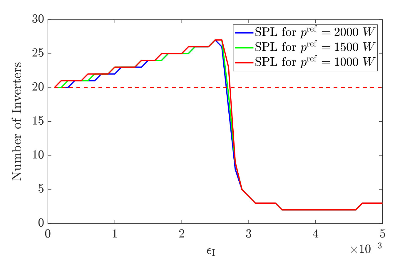 Figure 1
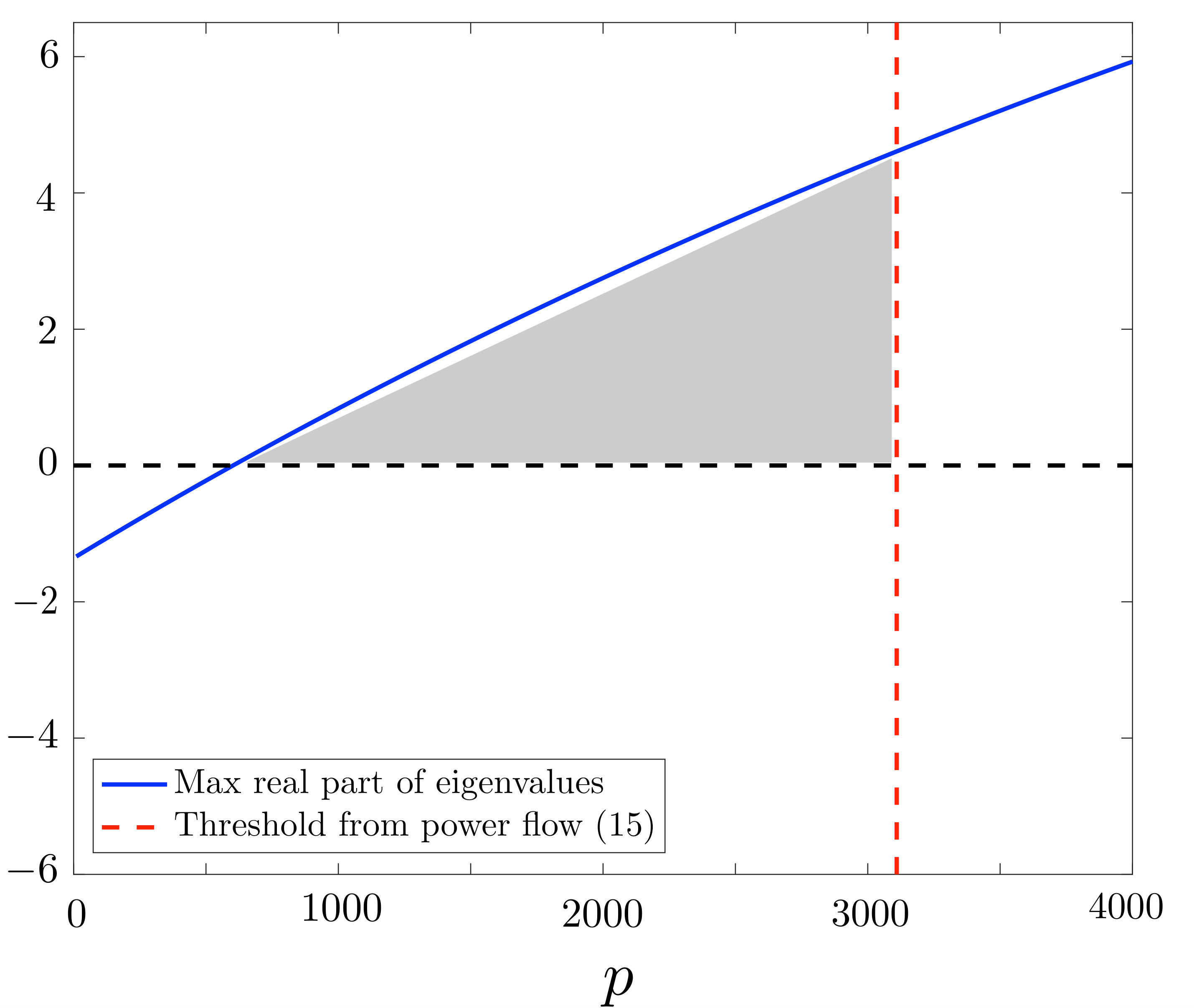 Figure 2
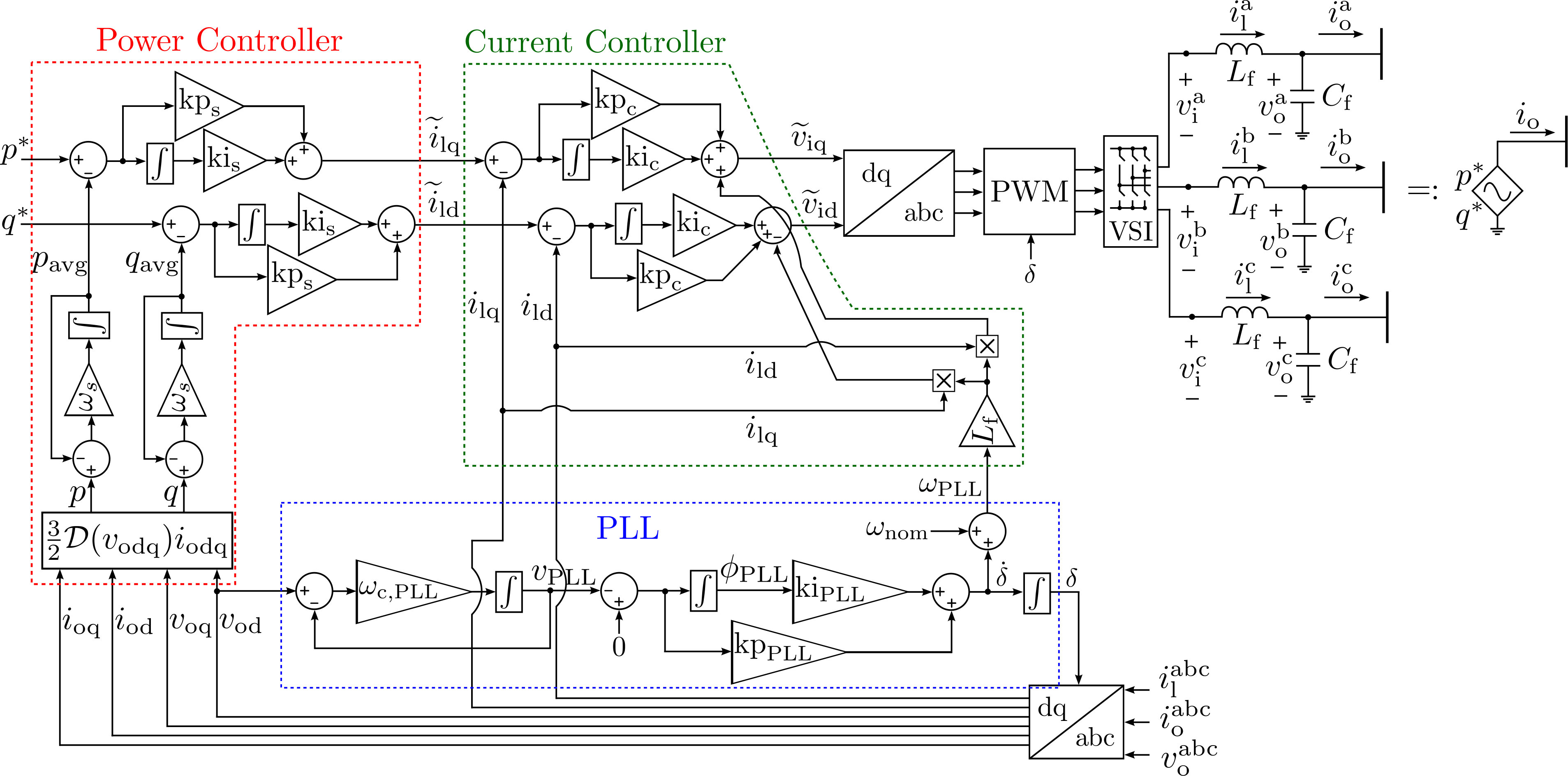 Figure 3
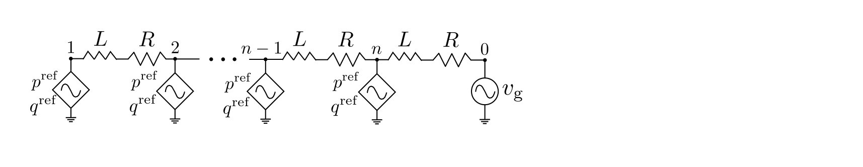 Figure 4
| 0.80 | 0.5853 | 0.0774 | 22 | 20 | 35 |
| 1.00 | 0.5636 | 0.0793 | 22 | 20 | 31 |
| 1.20 | 0.5546 | 0.0741 | 22 | 20 | 28 |
| 1.40 | 0.6525 | 0.0767 | 22 | 20 | 26 |
| 1.60 | 0.0767 | 0.5313 | 21 | 20 | 24 |
| 1.80 | 0.5063 | 0.0888 | 21 | 20 | 23 |
| 2.00 | 0.5241 | 0.0766 | 21 | 20 | 22 |
| Variable | Symbol | Variable | Symbol |
|---|---|---|---|
| PLL low-pass filter state | Current controller auxiliary state | ||
| PLL PI controller state | Current controller output voltage | ||
| PLL phase output | Output current | ||
| Power controller low-pass filter state | Power controller auxiliary state | ||
| Reference power injection | Current controller reference current | ||
| Power controller auxiliary state | PLL Frequency | ||
| Current in the lines | LC-filter voltage | ||
| Grid voltage | Grid frequency |
| Parameter | Symbol | Values from [24] | Values from [17] |
|---|---|---|---|
| Grid frequency | rad/s | rad/s | |
| Grid voltage amplitude | V | V | |
| PLL time constant | |||
| PLL time constant | |||
| PLL time constant | |||
| Power controller time constant | |||
| Power controller time constant | |||
| Power controller time constant | |||
| Current controller time constant | |||
| Current controller time constant | |||
| LC time constant | |||
| LC time constant | |||
| Line time constant | |||
| Line time constant |
Peer Reviews
No public reviews on file for this paper yet. If you reviewed it on a platform where reviews are public (OpenReview, ICLR, NeurIPS, ICML), you can paste yours below so the community can read it here.
Videos
No videos yet. Explain this paper in a talk, walkthrough, or lecture? Add one.
Singular Perturbation and Small-signal Stability
for Inverter Networks
Saber Jafarpour, Victor Purba, Brian B. Johnson,
Sairaj V. Dhople, and Francesco Bullo S. Jafarpour and F. Bullo are with the Center of Control, Dynamical Systems and Computation, University of California Santa Barbara, CA 93106, USA. E-mail: (saber.jafarpour, [email protected]).V. Purba and S. V. Dhople are with Department of Electrical and Computer Engineering at the University of Minnesota, Minneapolis, MN 55414 USA. E-mail: (purba002, [email protected]).Brian B. Johnson is with the Department of Electrical Engineering at University of Washington, Seattle, Washington, WA 98195 USA. E-mail: ([email protected])
Abstract
This paper examines small-signal stability of electrical networks composed dominantly of three-phase grid-following inverters. We show that the mere existence of a high-voltage power flow solution does not necessarily imply small-signal stability; this motivates us to develop a framework for stability analysis that systematically acknowledges inverter dynamics. We identify a suitable time-scale decomposition for the inverter dynamics, and using singular perturbation theory, obtain an analytic sufficient condition to verify small-signal stability. Compared to the alternative of performing an eigenvalue analysis of the full-order network dynamics, our analytic sufficient condition reduces computational complexity and yields insights on the role of network topology and constitution as well as inverter-filter and control parameters on small-signal stability. Numerical simulations for a radial network validate the approach and illustrate the efficiency of our analytic conditions for designing and monitoring grid-tied inverter networks.
Index Terms:
networks of inverters, dynamical system analysis, stability analysis
I Introduction
Problem description and motivation
The ongoing shift from fossil-fuel-driven synchronous generators to power-electronics-interfaced renewable energy is leading to changes in how power grids are modeled, analyzed, and controlled. While synchronous generators are generally rated at several hundreds of MVA and installed on the transmission backbone, power electronics inverters are distributed across both transmission and distribution subsystems and are generally much smaller in capacity. Furthermore, synchronous generators have large rotating masses that buffer supply-demand fluctuations and limit frequency excursions during transients, whereas inverters have very different dynamics (attributable dominantly to output filters and digital controllers [30]) and they possess no moving parts. Future grids will have large number of power-electronics-interfaced generations with highly distributed architecture as inverters assume a more prominent role, and this will necessitate the development of compatible models and computationally efficient analysis approaches to certify stability.
Most commercial inverters on the market for residential and utility-scale applications are grid-following. This means inverters inject currents while synchronized to the voltage at their terminals which is assumed to be set externally by the bulk grid. In effect, grid-following inverters act as voltage-following current sources. In recent years, there has been increased attention on grid-forming inverter technology, whereby—much like conventional synchronous generators—terminal voltage and frequency are modulated as a function of real- and reactive-power injections. Indeed, while grid-forming technology may very well be the solution for grids with penetration levels approaching , in the foreseeable future, it is likely that the bulk grid will see conventional synchronous generators co-exist alongside a large number of grid-following inverters. For instance, in Oahu, Hawaii, at least micro-inverters interconnect photovoltaic panels to the grid, producing as much power as the state’s largest conventional power plant, Konkar [9]. This motivates the problem of stability analysis for large-scale networks composed dominantly of grid-following inverters that we examine in this work.
The inverter dynamical model that we investigate is composed of a current controller, a power controller, a PLL, and an LCL filter. This is prototypical and mirrors models published widely in the literature [16, 17, 18, 19, 20, 23, 24, 27]. We propose a framework that leverages singular perturbation methods to obtain an analytic, computationally light-weight condition for small-signal stability assessment of three-phase distribution networks with grid-following inverters. Our solution strategy yields an analytic condition for stability that is agnostic to system size and clearly highlights the role of the network topology and pertinent system parameters on system stability. Due to the complexity of the involved dynamics, most prior art on stability of inverter-based systems has typically focused on simplified models that neglect inner control loops which underpin fast dynamics [26] (see the discussions in [5]). Some exceptions are [1, 31], where stability of full-order inverter models are studied in grid-connected networks. However, these studies are restricted to parallel networks of inverters and are not applicable to networks with general topologies. In some cases, detailed inverter models have been considered in general networks, but system stability has only been studied for a single inverter or a small network of inverters using numerical eigenvalue analysis. For instance, small-signal stability is analyzed in the literature using eigenvalue analysis for a single grid-following inverter under unintentional islanding in [28], for the IEEE -bus system with inverters in [23, 24], for a radial network consisting of inverters in [17], and for a single-machine-single-inverter network in [14]. Understandably, while numerical eigenvalue analysis of the linearized network is indeed a reasonable strategy, this approach comes with significant drawbacks. First, the large size of the network combined with the high dimensionality of the inverter model pose computational challenges to analysis. Furthermore, studying small-signal stability by computing eigenvalues of the linearized system does not reveal the role of critical network attributes on system stability, insights, which if formalized appropriately can facilitate analysis and design.
On a tangential note, it must be acknowledged that there is a growing body of work on stability assessment of synchronous generators and grid-forming inverter systems, and this includes approaches that have applied model-order reduction using singular perturbation analysis. For instance, in [6, 10], a model-reduction approach based on singular perturbation is proposed to study stability and control of grid-forming inverters. In [15], singular perturbation is applied to obtain a hierarchy of reduced-order models for inverters in the grid-forming mode. In [24], a suitable time-scale decomposition for a class of inverters is identified and an iterative scheme for model order reduction is proposed. We refer interested readers to [25] for a survey on singular perturbation methods and to [26] for a survey on application of singular perturbation in stability and control of inverters.
Contributions
We make several contributions to the study of small-signal stability of grid-following inverter networks. First, we show that adopting a static model for grid-following inverters (as fixed sources of active and reactive power) and neglecting fast dynamics induced by the inverters’ control loops may lead to erroneous conclusions regarding stability (see Example 3). This underscores the importance of acknowledging a full-order model for stability analysis. We start by introducing a model for grid-tied inverter networks that acknowledges line dynamics and where each inverter is modeled using a th-order model. Next, we uncover a correspondence between the equilibrium points of the dynamics and the solutions of the algebraic power-flow equations. The main contribution of this paper, i.e., an analytic sufficient condition for small-signal stability, is derived in the context of a dimensionless transcription of the involved models which leads to the identification of a physically insightful parametrization of the inverters. We show that certain assumptions on the range of parameters result in a time-scale decomposition of the system. Using singular perturbation analysis, we propose an analytic sufficient condition which guarantees small-signal stability over a given parametric regime. As a unique contribution, we emphasize that the dimensionless form of the network equations as well as the regularity of the singular perturbation problem (i.e., existence of isolated quasi-steady state manifolds) are critical steps in a rigorous time-scale analysis. Over this specified parametric regime, our analytic sufficient condition can also be interpreted as a lower bound on the stability threshold of the network and allows us to check system stability with minimal computational complexity. Furthermore, in the special case of resistive networks, our sufficient condition reduces to checking Hurwitzness of a Metzler matrix, something that can be implemented efficiently via linear programming (see [22]).
In the literature, small-signal stability of systems is usually studied using eigenvalue analysis for the full-order models (e.g., see [17]) or for the reduced-order models (e.g., see the survey [26]). Compared to performing eigenvalue analysis for the full-order system, our proposed analytically driven sufficient condition reduces computational complexity by addressing the high dimensionality of the underlying dynamics (the inverter model we study has dynamical states) and it demarcates the role of the network (topology and constitution) and pertinent inverter dynamics (filter and controller parameters). Moreover, while many existing approaches in the literature only outline iterative schemes for model reduction (see [24]), our analysis provides an explicit reduced-order model. Finally, we provide several numerical case studies that validate the analysis.
Paper organization
In Section II, we present the dynamical model for a class of three-phase grid-following inverters. In Section III, we derive an equivalent dimensionless description for a grid-tied network of inverters and loads and we study the equilibrium points of the system. In Section IV, we provide a sufficient condition for existence of a locally exponentially stable equilibrium point. Finally, in Section V, we illustrate some applications of the theoretical results in network design and stability assessment.
Notation
Vectors and matrices. We denote the set of real numbers by , the set of complex numbers by , the set of complex numbers with negative real part by , the set of binary -tuples by , and the -dimensional torus by . We define . We identify the complex plane with the real plane . For a complex number , the norm of is and the argument of , , is the angle between and the positive imaginary axis. We denote the identity matrix of dimension by , the -column vector of zeros with , and the -column vector of ones with . For a matrix , we denote the trace by , the determinant by , and -norm by . For two real symmetric matrices we write if is positive definite. A real square matrix is Metzler if all its off-diagonal entries are non-negative. For two square matrices and , the tensor product is denoted by . For a vector , we denote by .
From -complex variables to -real variables. For every complex , the associated real variable in the real plane is denoted by . We will frequently use matrix , matrix , and the rotation matrix (parameterized by angle ) by . Let . We define matrix-valued operators and by
[TABLE]
All the above matrices and operators can be extended to the -dimensional complex and -dimensional real spaces using block diagonal structure. For the brevity of notation, we denote the extended -dimensional complex (-dimensional real) matrix/operator with the same symbol as its -dimensional complex (-dimensional real) counterpart. Let and be the associated real vector, then we define .
Algebraic graph theory. We denote an undirected weighted graph by a triple , where is the set of nodes and is the set of edges. The matrix is the weighted adjacency matrix. For every node , the degree of the node is given by . For a fixed orientation on , the incidence matrix of the graph is denoted by . The Laplacian for the graph is defined by , where .
Power systems. We consider two different reference frames. The first is the so-called global -frame, and it is a rotating reference frame tied to the nominal grid frequency . The second frame, which is usually referred as the local -frame, is with reference to each inverter’s terminal voltage vector. For a balanced three-phase signal , we denote the -frame representation by and the -frame representation by . These are related as follows: , where is the angle between the -frame and the -frame. We assume that all the electrical signals in the network are balanced [2, Chapter 2]. Therefore, the voltage of the grid is a three-phase AC signal given by the time-varying function and in the global -frame, it is represented as , where is the amplitude of the grid voltage.
II Model of Individual Inverter
We briefly overview the dynamics of the type of grid-following -phase inverters examined in this work. For a more detailed description of the model, see [20, 23]. The model captures all relevant AC-side dynamics, and is composed of a: i) phase-locked loop (PLL), ii) power controller, iii) current controller, and iv) output filter. An illustrative block diagram is given in Fig. 1.
The PLL consists of a low-pass filter with cut-off frequency and a PI controller with gains and . The PLL dynamics are
[TABLE]
where and denote states of the low-pass filter and PI controller, respectively, is the output of the PI controller, and is the -component of the output voltage of the inverter. The frequency of the PLL loop is defined by . The power controller consists of two low-pass filters with cut-off frequency and two PI controllers with gains and . The pertinent dynamics are given by:
[TABLE]
where collects the states of the low-pass filters, capture the outputs of the PI controllers (these are the references for the current controller), collects the active- and reactive-power references, and collects instantaneous active- and reactive-power outputs (measured at the point of common coupling):
[TABLE]
The current controller consists of two PI controllers with gains and , with outputs to be the references for the inverter voltage at the switching terminals :
[TABLE]
Since the switching period is typically much shorter than the filter and controller time constants, we assume that . The dynamics of the filter are given by
[TABLE]
Finally, we introduce two new variables , and , that will aid in exposition. The inner- and outer-loop control architecture examined here is ubiquitous, see, e.g., [16, 17, 18, 19, 20, 23, 24, 27], where similar models are utilized.
Now, we write the dynamical system of the inverters in the global -frame. To this end, we introduce:
[TABLE]
For vector with time-varying entries, the time derivatives in the global -frame and local -frame are related by
[TABLE]
Leveraging this identity, the dynamical model for the grid-following inverter in the -frame can be expressed as:
[TABLE]
where captures states of the inverter in the global reference frame, captures the references for active and reactive power, is the drift vector field, and , and are control vector fields. The mappings and the matrix are obtained from the dynamics governing the current controller, the power controller, the PLL, and the filter outlined previously.
III Model for Grid-tied Network of Inverters
In this section, we derive the dynamical system model governing the grid-tied network of inverters and loads and study the equilibrium points of the system. We model the network using an undirected, connected, complex-weighted graph with node set (buses) , edge set (branches) , and the symmetric matrix-valued edge weights (admittances) , where is the resistance and is the inductance of the line , for every . Suppose is the incidence matrix of . There are three types of nodes in the network: we have one grid bus with voltage denoted by [math]. We have inverter buses collected in the set , and load buses collected in the set . Without loss of generality, we assume that and such that . Therefore and we assume that . Associated to the matrix-weighted graph, , we define the nodal admittance matrix by , where is given by . The partition induces the following decomposition of incidence matrix : , where , , and , and the following partition for the admittance matrix :
[TABLE]
We also establish the following convention: for a given variable (parameter) corresponding to the inverter, we define vector , where is the associated variable (parameter) for the th inverter.
Inverter model
Using (5), the governing dynamics for all inverters in the network can be expressed as:
[TABLE]
where, in , captures all the dynamic states for the th inverter, , , and , where is the drift vector field and and are control vector fields of inverter .
Load and line models
Let be the th load voltage (in the -frame) and be the current demand (in the -frame) of the th load. We collect the nodal voltages and current demands for the loads in and , respectively. We assume loads are purely resistive; suppose is the vector of load resistances, then the loads can be described by
[TABLE]
Suppose that the vector of line resistances and line inductances are denoted by and , respectively; the nodal current injections by and nodal voltages by . The governing dynamics for the transmission lines are [26, Equation 4.10]:
[TABLE]
where is the vector of current flows in the lines. Thus we have .
III-A Network Model and Dimensionless Transcription
From (6)–(8), the grid-tied inverter-network dynamics are:
[TABLE]
where and \mathbf{v}_{\textup{L}}=\big{(}-B_{\textup{L}}[\mathbf{R}_{\textup{L}}]\otimes I_{2}\big{)}\xi_{\textup{DQ}}. We transcribe the differential equations (III-A) in a dimensionless format. We assume that is the nominal power generation/consumption in the network. For each inverter, we introduce the following dimensionless variables:
[TABLE]
For the network, we introduce the dimensionless parameters
[TABLE]
We also isolate time-constants of different sub-systems:
- •
for the PLL low-pass filter: and ;
- •
for the PLL PI controller: ;
- •
for the low-pass filter of the power controller: ;
- •
for tracking in the power controller: ;
- •
for the PI controller in the power controller: ;
- •
for the current controller: ;
- •
for the PI controller in the current controller: ;
- •
for the LC filter: and and ;
- •
for line in the network: and .
With these preliminaries in place, the dimensionless grid-tied inverter-network dynamics can be expressed as:
[TABLE]
Above,
[TABLE]
The dimensionless grid-tied inverter network dynamics (10a)–(10i) is -dimensional. Our first goal is to find the equilibrium points of the dynamical systems (10a)–(10i).
III-B *Equilibrium points of the Dimensionless Grid-tied
Inverter-network Dynamics*
We start by introducing some notation. Let be the admittance matrix of the network. Then
[TABLE]
and the dimensionless parameters:
[TABLE]
We show that the equilibrium points of the dimensionless grid-tied inverter network dynamics (10) are in correspondence with the solutions of the following power-flow equations:
[TABLE]
Lemma 1**.**
For a given reference-power injection to the inverters, the following statements are equivalent:
- (i)
* is a solution for the power-flow equations (12) and (13);* 2. (ii)
for every , is an equilibrium point of the dimensionless grid-tied inverter-network dynamics (10) given by
[TABLE]
with
[TABLE]
Proof.
Regarding , from the power-controllers’ dynamics in (10), we can conclude that if is an equilibrium point, then we have . This implies satisfies (12). Moreover, at the equilibrium point , the line dynamics (10i) will simplify to . Using Kron reduction [8], this implies that satisfies (13).
Regarding , suppose is a solution to the power flow equations (12) and (13). Then from the PLL dynamics in (10), we have and . Note that, can be written in the trigonometric form
[TABLE]
This implies that, for every , there exists such that . From the power-controller dynamics in (10), we have . Finally, one can find the value of , , , and by solving the remaining equations in (10). ∎
Remark 2**.**
The power-flow equations (12) and (13) have been studied extensively in the literature and many sufficient conditions for existence and uniqueness of solutions have been developed; see, e.g., [3, 7, 29]. Lemma 15 in Appendix C restates a result from [29] pertaining to uniqueness that is leveraged in subsequent results.
IV Stability Analysis of the Dimensionless Grid-tied Inverter-network Dynamics
In bulk power-systems dynamics literature, it is commonplace to assume that the dynamics of the grid-following inverters are much faster than the dynamics of grid-forming inverters and synchronous machines [26]. This assumption justifies the use of a static model for grid-following inverters such that the inverter nodes are considered to be sources of constant (active and reactive) power. Subsequently, the network operation is described by the following power-flow equations:
[TABLE]
Quite obviously, the static representation (14) does not capture stability. The following example shows that the internal dynamics of the inverters can induce instabilities, even if the power-flow equations in (14) admit a high-voltage solution.
Example 3**.**
(Instabilities Induced by Inverter Dynamics)* Consider the radial grid-connected network consisting of identical inverters (a sketch is provided in Fig. 2). Suppose the inverters have uniform reference power injections , each line has resistance and inductance , and the grid voltage is with constant frequency .*
- (i)
Static model:* If inverter power injections satisfy*
[TABLE]
then, there exists a unique high-voltage, low-current solution for the power-flow equations (14) (see Lemma 15). 2. (ii)
Dynamic model:* We use the dynamic model (5) for the inverters (parameters are given in the fourth column of Table III). The governing equations for the network are in (10), and condition (15) via Lemma 1 guarantees the existence of a family of equilibrium points , for the system (10). Linearizing the system (10), we study local stability of the equilibrium point .*
Figure 3 plots the maximum real part of the eigenvalues of the linearized system (10) around the equilibrium point as a function of active-power injection. The red vertical line is the threshold of the power injection for which the power-flow equations admit a unique solution (obtained from (15)). Notice that there are power injections for which a high-voltage solution of the power-flow equations exists, however, the corresponding equilibrium point is not stable.
IV-A Small-signal Stability via Time-scale Separation
We now focus on the small-signal stability of the dimensionless grid-tied inverter-network dynamics (10). Due to high dimensionality and nonlinearity of the dynamic model, studying small-signal stability is not analytically tractable. Therefore, it is a reasonable goal to reduce the model order. To that end, we identify a physically meaningful parametrization of the inverters, and we show that under suitable assumptions, this parametrization leads to a time-scale decomposition of the system (10) which simplifies analysis. We begin by uncovering time constants of different sub-systems.
Definition 4** (Singular perturbation parameter).**
For dynamics (10), we define:
[TABLE]
Using these, we define the singular perturbation parameter:
[TABLE]
Remark 5**.**
- (i)
Definition 4 establishes a physically meaningful time-scale separation of the components of the inverter network when . In this case, which implies that the line dynamics, the filter, and the current controller of the inverter are the fastest components of the network. Moreover, which implies that the PLL, and averaging-part of the power controller (i.e., ) are slower than the current controller, the line dynamics, and the filter but they are faster than the steady-state power-tracking controller (i.e., ) dynamics. 2. (ii)
The assumption is equivalent to , which is realistic in practice. For instance, in the inverter models with the parameters in Table III and with the parameters used in **[17, 23, 24]**, it holds that . 3. (iii)
, for every . Similarly, one can show that and this gives an upper bound for the LC and line parameter . 4. (iv)
For a different set of parameters and control architectures, one can conceivably identify a different singular perturbation parameter and time-scale decomposition. However, we expect the general nature of the stability result that follows to be similar.
Theorem 6** (Small-signal Stability).**
Consider the dimensionless grid-tied inverter-network dynamics (10) with states in and references . The following hold:
- (i)
if,
[TABLE]
then, there is a unique solution for the power-flow equations (12) and (13) and a family of equilibrium points , , for the grid-tied inverter network dynamics (10) satisfying:
[TABLE] 2. (ii)
if additionally, and the matrix
[TABLE]
is Hurwitz, then, there exists an such that, for every , the equilibrium point is locally exponentially stable.
Proof.
Regarding part (i), the proof follows from combining Lemma 15 and Lemma 1. Regarding part (ii), consider the dimensionless grid-tied inverter network dynamics (10). Using (16) and defining the variable by , we get a three-time-scale decomposition of the system. We define the states , , and as follows:
[TABLE]
where is faster than and are faster than . The corresponding time-scales are given by and . Using these time scales, the dimensionless grid-tied inverter network dynamics (10) can be written as follows:
[TABLE]
where are suitably defined functions. The quasi-steady-state manifold for the time-scale is the manifold obtained by solving the algebraic equations [12, §11.2]. After some algebraic computations, the quasi-steady-state manifold for the time-scale is time-invariant and is given by:
[TABLE]
Since the quasi-steady state manifold for the time-scale is an isolated manifold, the singular perturbation problem is in the standard form. The boundary-layer dynamics are:
[TABLE]
We first show that for the boundary-layer dynamics (20), the origin is the exponentially stable equilibrium point. It is easy to see that since the graph is connected, we have , the matrix is skew-symmetric and the matrix is negative definite. Hence, using Lemma 14, the origin is the locally exponentially stable point of the boundary-layer dynamics (20). Similarly, the quasi-steady-state manifold for time-scale is obtained by solving the algebraic equations . Thus, the quasi-steady-state manifold for time-scale is time-invariant and is given by:
[TABLE]
where is the solution to:
[TABLE]
Since the quasi-steady state manifold for the time-scale is an isolated manifold, the singular perturbation problem is in the standard form with boundary-layer dynamics:
[TABLE]
We show that the boundary-layer dynamics (21) are stable around the origin. Note that the linearized boundary-layer equation dynamics around the origin have the form , where has the upper block triangular form with:
[TABLE]
Since , by Lemma 14, matrix is Hurwitz. Therefore, the origin is the locally exponentially stable point of the boundary-layer equations (21). Now, we consider the reduced-order dynamics. The reduced-order model for the multi-time-scale analysis is given by:
[TABLE]
In order to study the stability of the reduced-order model (22), we introduce the new variable . First note that, for , we have and . This implies that and the reduced order model (22) is given by:
[TABLE]
Linearizing the above equation, we get , where
[TABLE]
Note that, for any scalar and any matrix , the matrix is Hurwitz if and only if the matrix is Hurwitz. Moreover, by [11, Theorem 1.3.22], Hurwitzness of the matrix is equivalent to the Hurwitzness of matrix defined in (18). This means that is Hurwitz and the origin is a locally exponentially stable equilibrium point of the reduced-order model (22). Stability of the equilibrium point of the dimensionless grid-tied inverter network dynamics follows from condition (ii) [12, Theorem 11.4].∎
We provide a few contextualizing and clarifying remarks.
Remark 7**.**
- (1)
It is well-known in singular perturbation analysis that the largest value of for which Theorem 6(ii)* holds is hard to compute. A standard lower bound on can be obtained using techniques in [13, Lemma 2.2].* 2. (2)
Small-signal stability analysis of the grid-tied inverter network dynamics (10) is computationally complicated for large networks and, in general, it requires linearizing the system (10) and checking stability of a -dimensional matrix. Theorem 6(ii)* uses a time-scale analysis to eliminate the line dynamics, the dynamics of the current controller, PLL, and filter from small-signal stability analysis. The sufficient condition in Theorem 6(ii)** significantly reduces computational complexity by reducing the problem to checking that a -dimensional matrix is Hurwitz;* 3. (3)
By part (i), there exists a family of equilibrium point for the grid-tied inverter network dynamics (10). However, in part (ii), we focus on the equilibrium point . The reason is that this trajectory is locally exponentially stable when there is no power injection for the inverters; 4. (4)
Theorem 6(ii)* brings out the role of network topology, the power injections/demands, and inverter parameters in small-signal stability of inverter networks. For the matrix , the term reveals the role of network topology. The terms , , and (obtained by solving the power-flow equations (12)–(13)) reveal the role of network topology and power injections/demands. Finally, reveals the role of inverters’ internal dynamics.*
IV-B Corollaries
We now present two corollaries that may be applicable in different settings and shed more light on to the main result.
Corollary 8** (Single inverter connected to the grid).**
Consider a single inverter with the reference power injection connected to the grid with voltage through a line with resistance and inductance . If
[TABLE]
then the following statements hold:
- (i)
there exist two equilibrium points and satisfying
[TABLE] 2. (ii)
if we have , then there exists a such that, for every , is locally exponentially stable.
Proof.
Regarding part (i), we define the dimensionless resistance and dimensionless inductance . Therefore, we get . Then, (23) is equivalent to (17) and the result follows from Theorem 6(i). Regarding part (ii), note that we have . Then, matrix in (18) becomes:
[TABLE]
Using simple algebraic manipulations, we get and . Since , we have . This implies that . Moreover, for the equilibrium points , we have . This implies that and is Hurwitz. Thus, by Theorem 6(ii), is locally exponentially stable. ∎
In the next corollary, we study the special case of resistive networks and provide a computationally efficient numerical method for checking sufficient condition (18).
Corollary 9** (Resistive network of inverters).**
Consider the dynamics (10). Suppose the lines are purely resistive and the reference power injections and demands are purely active. The following statements hold:
- (i)
if , where , then there exists a family of equilibrium points for (10) with the property that
[TABLE] 2. (ii)
if additionally and the Metzler matrix
[TABLE]
is Hurwitz, then there exists such that for every , equilibrium is locally exponentially stable.
Proof.
Regarding part (i), since the network is resistive and power injections/demands are purely active, we know that
[TABLE]
Therefore: . The result then follows from Theorem 6(i). Regarding part (ii), since there are no reactive-power injections from the inverters, we have . Since the input voltage for the PLL and power controller is the output voltage of the filter (i.e., ), and the network is purely resistive, we have and as a result . Alternatively, this observation can be proved rigorously as follows. Since the power injections are purely active, the power injection vector has the form . Therefore, starting from the initial condition , the th iteration in Lemma 15(ii) has the form , for every integer . This implies that, in the limit, we have and as a result . Therefore, the matrix in condition (18) simplifies as shown below:
[TABLE]
Using Lemma 13, matrix is Hurwitz if and only if matrices
[TABLE]
are Hurwitz. Note that the active-power injections from the inverters to the grid are non-negative in steady state. This implies that . Thus, the matrices (25) are similar to the following matrices:
[TABLE]
Since the matrix is positive definite and the matrix is positive semidefinite, the matrix
[TABLE]
is Hurwitz. Moreover, note that the matrix is a grounded Laplacian matrix and by [4, E 9.10] its inverse is non-negative. Also, the matrices , , and are all diagonal with non-negative diagonal elements. This implies that the matrix has non-negative off-diagonal elements and therefore, it is Metzler. The proof of Corollary (9) then follows from Theorem 6. ∎
Remark 10** (Computational complexity).**
There are computationally efficient methods for checking Hurwitzness of Metzler matrices. In particular, one can reformulate the Hurwitzness of (24) as the following feasibility problem:
[TABLE]
The feasibility problem (26) is a linear program and can be checked using distributed methods whose computational time scales linearly with the number of non-zero elements in [22].
V Numerical Simulations
In this section, we present numerical simulation results for radial networks (see Fig. 2) with identical inverters and reference-power setpoints with the goal of answering the following questions:111All the numerical simulations are performed in MATLAB R2016a on a computer with Intel Core i5 processor CPU and RAM.
- •
For which values of the inverter parameter does Theorem 6(ii) guarantee small-signal stability?
- •
How efficient is the condition (18) in Theorem 6(ii) to analyze small-signal stability?
The first question can be interpreted as an inverter design problem, while the second question can be interpreted as a network monitoring problem. Solutions to these problems are provided in Sections V-A and V-B, respectively. Our test case is a family of radial networks , where is the weighted undirected connected graph with the node set (buses) and the edge set (branches) (see Fig. 2). For every radial network , the node [math] is the slack bus connected to the grid with voltage and frequency . Nodes are the inverters with , and
[TABLE]
For every , the admittance of line is given by , where the line resistance is and line inductance is . We first define the notion of a safe penetration level.
Definition 11** (Safe Penetration Level).**
Given a family of networks and uniform reference power injection , the Safe Penetration Level (SPL) for is the maximum such that the dimensionless grid-tied inverter network dynamics (10) with underlying graph and reference powers has a locally stable equilibrium point.
Remark 12**.**
- (1)
For our test case network, SPL of the network depends on the parameter ; 2. (2)
One can use the matrix defined in (18) to estimate the SPL of the network; from Theorem 6(ii)**, there exists such that, for every , SPL of the network is larger than this estimate.
V-A Designing Grid-tied Inverter Networks
In this part, we examine the efficiency of our analytic results in Theorem 6 to design grid-following inverter networks focusing on the small-signal stability of the grid. In particular, we focus on estimating the SPL for the radial network shown in Fig 2 and numerically computing the largest range of parameter for which Theorem 6(ii) holds. In order to carry out this task, we study the effect of parameter for different active power injections on the SPL of the system. The result is shown in Fig. 4.
Note that the overlapping dashed lines in Fig. 4 are the estimates of SPL based on the sufficient condition in Theorem 6(ii). Therefore, according to the data in Fig. 4, the largest domain of the inverter parameter for which Theorem 6(ii) holds is , for the active power injections , , and , respectively. It is interesting that, as becomes smaller, the dashed line and the solid lines get closer to each other and Theorem 6(ii) can be used to find the exact SPL of the network.
V-B Monitoring Grid-tied Inverter Networks
In this section, we study the accuracy and computational efficiency of condition (18) in Theorem 6(ii) for monitoring the small-signal stability of the network. For our test case, we pick the parameter . Therefore based on the discussion in Section V-A, we are in the range of applicability of Theorem 6(ii). Recall that SPL is the largest number of inverters in the network for which the equilibrium point of full-order system (10) is locally asymptotically stable. We denote the computational time of finding SPL, using the eigenvalue analysis for the linearized system, by . We denote the largest number of inverters in the grid for which the matrix in (18) is Hurwitz by . Similarly, we denote the computational time for checking the Hurwitzness of matrix in (18) by . Finally, we denote the largest number of inverters in the grid for which condition (15) holds, by . We start with different uniform reference active-power injections and compute the thresholds , , and together with the computational times for and , for each active-power injections. The results are shown in Table I. From Table I, one can see that the static condition (15) overestimates the value of . Moreover, it is clear that condition (18) gives an accurate lower bound for safe penetration level and its corresponding computation time (i.e., ) is almost one order of magnitude less that the computation time to perform eigenvalue analysis for the full-order system (i.e., ).
VI Conclusion
We studied small-signal stability of grid-tied networks of grid-following inverters and loads. Using a time-scale analysis and a suitable choice of a family of parameters for the inverters, we presented an analytic sufficient condition for local exponential stability. We showed that, compared to the direct eigenvalue analysis of the full-order system, this sufficient condition has the advantages of reducing the computational complexity of checking small-signal stability as well as providing insights about the role of the network topology and inverter parameters on stability.
Appendix A Table of variables and parameters
Table (II) collects the variables and their symbols for grid-following inverter model and Table (III) collects the parameter values for this class of inverters.
Appendix B Pertinent Results from Linear Algebra
Lemma 13**.**
Let be the eigenvalues of a matrix . For , is an eigenvalue of if and only if it is an eigenvalue of , for some .
We omit the proof of this elementary result.
Lemma 14**.**
Let and be diagonal matrices with positive diagonal entries such that . Suppose that is an arbitrary matrix with , is a skew-symmetric matrix, and is such that is negative definite. Then the following matrices are Hurwitz:
[TABLE]
Proof.
The characteristic polynomial of matrix is: . Since all matrices , , , and are diagonal, is an eigenvalue of if and only if . The diagonal elements of the matrices , , , and are positive. Therefore, using the Routh–Hurwitz criteria, if and only if . Thus, is Hurwitz if and only if . To show that the matrix is Hurwitz, we use LaSalle’s invariance principle [12, Theorem 4.4]. Consider the dynamical system , where . We define the Lyapunov function by: V(\mathrm{x}_{1},\mathrm{x}_{2},\mathrm{x}_{3},\mathrm{x}_{4})=\tfrac{1}{2}\big{(}\mathrm{x}_{1}^{\top}\Gamma^{-1}\mathrm{x}_{1}+\mathrm{x}_{2}^{\top}\Xi^{-1}\mathrm{x}_{2}+\mathrm{x}_{3}^{\top}\Pi^{-1}\mathrm{x}_{3}+\mathrm{x}_{4}^{\top}\Theta^{-1}\mathrm{x}_{4}\big{)} Then, it is easy to check that . Therefore, by LaSalle’s invariance principle, the trajectories of the system converges to the largest invariant set inside . It is easy to see that . Let us denote the largest invariant set inside by . Our goal is to show that . Suppose that is a trajectory which belongs identically to . Then we have . First note that implies that . Since , we deduce that . Moreover, we see that . This implies that . Thus, the only invariant set inside is and thus is Hurwitz. ∎
Appendix C Solutions to power flow equation
Lemma 15**.**
Consider (12) and (13) with . Suppose
[TABLE]
Then the following statements hold:
- (i)
the power flow equations (12) and (13) has a unique solution with , where
[TABLE] 2. (ii)
for every , the iteration procedure
[TABLE]
converges to , where is the unique solution to (12) and (13).
Proof.
By considering , part (i) and (ii) are straightforward generalizations of [29, Theorem 1]. One should note the fact that the nodal variables in [29, Theorem 1] are average power injections/demands and therefore the power flow equations have the form . However, in this paper, the nodal variables are instantaneous power injections/demands and the power flow equations read . ∎
The reference list from the paper itself. Each links out to its DOI / PubMed record.
- 1[1] J. L. Agorreta, M. Borrega, J. López, and L. Marroyo. Modeling and control of N 𝑁 N -paralleled grid-connected inverters with LCL filter coupled due to grid impedance in PV plants. IEEE Transactions on Power Electronics , 26(3):770–785, 2011. doi:10.1109/TPEL.2010.2095429 . · doi ↗
- 2[2] H. Akagi, E. H. Watanabe, and M. Aredes. Instantaneous Power Theory and Applications to Power Conditioning . John Wiley & Sons, 2017, ISBN 978-0-470-10761-4.
- 3[3] S. Bolognani and S. Zampieri. On the existence and linear approximation of the power flow solution in power distribution networks. IEEE Transactions on Power Systems , 31(1):163–172, 2016. doi:10.1109/TPWRS.2015.2395452 . · doi ↗
- 4[4] F. Bullo. Lectures on Network Systems . Kindle Direct Publishing, 1.3 edition, July 2019, ISBN 978-1986425643. With contributions by J. Cortés, F. Dörfler, and S. Martínez. URL: http://motion.me.ucsb.edu/book-lns .
- 5[5] S. Y. Caliskan and P. Tabuada. Uses and abuses of the swing equation model. In IEEE Conf. on Decision and Control , pages 6662–6667, Osaka, Japan, December 2015. doi:10.1109/CDC.2015.7403268 . · doi ↗
- 6[6] S. Curi, D. Groß, and F. Dörfler. Control of low inertia power grids: A model reduction approach. In IEEE Conf. on Decision and Control , pages 5708–5713, Melbourne, Australia, December 2017. doi:10.1109/CDC.2017.8264521 . · doi ↗
- 7[7] S. V. Dhople, S. S. Guggilam, and Y. C. Chen. Linear approximations to AC power flow in rectangular coordinates. In Allerton Conf. on Communications, Control and Computing , pages 211–217, September 2015. doi:10.1109/ALLERTON.2015.7447006 . · doi ↗
- 8[8] F. Dörfler and F. Bullo. Kron reduction of graphs with applications to electrical networks. IEEE Transactions on Circuits and Systems I: Regular Papers , 60(1):150–163, 2013. doi:10.1109/TCSI.2012.2215780 . · doi ↗