Schur Algebras for the Alternating Group and Koszul Duality
Thangavelu Geetha, Amritanshu Prasad, Shraddha Srivastava

TL;DR
This paper introduces the alternating Schur algebra, explores its structure via bipartite graphs, and develops a combinatorial approach to Koszul duality for related modules, linking algebraic and graphical methods.
Contribution
It defines the alternating Schur algebra, provides a graphical basis, and connects Koszul duality with combinatorial techniques for modules over classical Schur algebras.
Findings
Graphical basis of $AS_F(n,d)$ in characteristic not 2
Characterization of $AS_F(n,d)$-modules via $S_F(n,d)$-modules
Dependence of Koszul duality behavior on parameters $n$ and $d$
Abstract
We introduce the alternating Schur algebra as the commutant of the action of the alternating group on the -fold tensor power of an -dimensional -vector space. When has characteristic different from , we give a basis of in terms of bipartite graphs, and a graphical interpretation of the structure constants. We introduce the abstract Koszul duality functor on modules for the even part of any -graded algebra. The algebra is -graded, having the classical Schur algebra as its even part. This leads to an approach to Koszul duality for -modules that is amenable to combinatorial methods. We characterize the category of -modules in terms of -modules and their Koszul duals. We use the graphical basis of to study the dependence of the behavior…
Click any figure to enlarge with its caption.
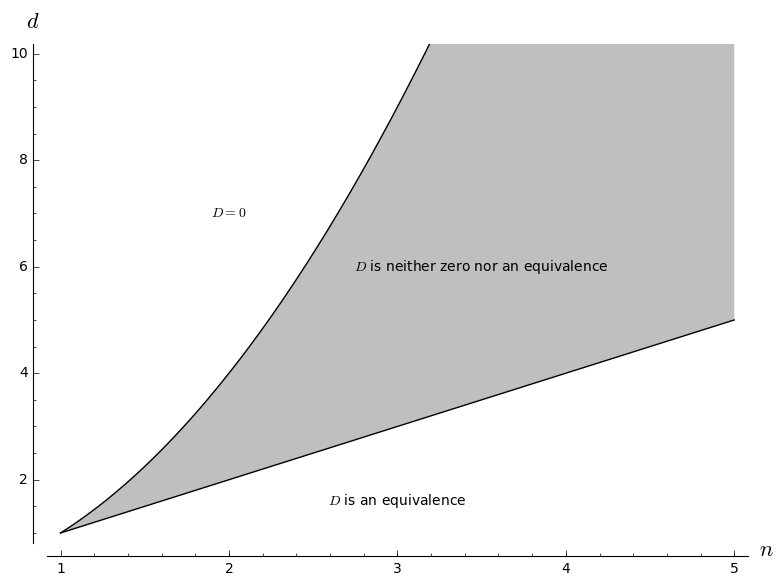 Figure 1
Peer Reviews
No public reviews on file for this paper yet. If you reviewed it on a platform where reviews are public (OpenReview, ICLR, NeurIPS, ICML), you can paste yours below so the community can read it here.
Videos
No videos yet. Explain this paper in a talk, walkthrough, or lecture? Add one.
Schur Algebras for the Alternating Group
and Koszul Duality
Thangavelu Geetha
Indian Institute of Science Education and Research, Thiruvananthapuram
,
Amritanshu Prasad
The Institute of Mathematical Sciences, HBNI, Chennai
and
Shraddha Srivastava
The Institute of Mathematical Sciences, HBNI, Chennai
Abstract.
We introduce the alternating Schur algebra as the commutant of the action of the alternating group on the -fold tensor power of an -dimensional -vector space. When has characteristic different from , we give a basis of in terms of bipartite graphs, and a graphical interpretation of the structure constants. We introduce the abstract Koszul duality functor on modules for the even part of any -graded algebra. The algebra is -graded, having the classical Schur algebra as its even part. This leads to an approach to Koszul duality for -modules that is amenable to combinatorial methods. We characterize the category of -modules in terms of -modules and their Koszul duals. We use the graphical basis of to study the dependence of the behavior of derived Koszul duality on and .
Key words and phrases:
Schur algebra, Koszul duality, Schur-Weyl duality, alternating group
2010 Mathematics Subject Classification:
20G43,20G05,05E10
1. Introduction
1.1. Schur-Weyl duality and its variants
Frobenius determined the irreducible characters of the symmetric group over , the field of complex numbers, in 1900 [12]. Building on this, Schur classified the irreducible polynomial representations of and computed their characters in his PhD thesis [27]. The group acts on the factors of , while permutes the tensor factors. In 1927, Schur used these commuting actions to reprove the results of his dissertation [28]. Following Weyl’s expositions of this method [32, 33], it is known as Schur-Weyl duality.
Over the years, several variants of Schur-Weyl duality have emerged. Shrinking to the orthogonal group , Brauer obtained the duality between Brauer algebras and [7]. Motivated by the Potts model in statistical mechanics, Jones [16] and Martin [20] further shrunk down to , obtaining the partition algebras . Bloss [5] reduced to to obtain an algebra which coincides with the partition algebra when . We take the smallest possible step in the opposite direction: we reveal what takes the place of the polynomial representations of when the action of the symmetric group is restricted to the alternating group . The situation is summarized in Table 1. The significance of this investigation lies in its connection with the Koszul duality functor on the category of homogeneous polynomial representations of of degree .
1.2. Schur algebras for the alternating group
Motivated by Green [14, Theorem 2.6c], define the Schur algebra as
[TABLE]
for any field , and positive integers and . When is infinite, then -modules are the same as homogeneous polynomial representations of of degree (see [14, Section 2.4] and [23, Section 6.2]). Define the alternating Schur algebra by replacing by in the definition above:
[TABLE]
When has characteristic different from , this algebra has a decomposition (Lemma 2.1)
[TABLE]
as a -graded algebra. Here , where denotes the sign character of . The subspace is an-bimodule.
When , then , and , as observed by Regev [25, Theorem 1]. But when , , and in Lemma 2.2, we note that is a full tilting left -module as studied by Donkin in [9, Section 3].
1.3. Bases and structure constants
Schur [28] gave a combinatorial description of a basis and the corresponding structure constants of the Schur algebra (see also [14, Section 2.3]). By indexing Schur’s basis of by bipartite multigraphs with vertices and edges, Méndez [22] (see also Geetha and Prasad [13]) gave a graphic interpretation of the structure constants. We describe a basis of in terms of bipartite simple graphs in Theorem 2.24. So from the decomposition (1), a basis of is obtained. A graphic interpretation of the structure constants of is given in Theorems 2.14 and 2.25. This will be used to derive properties of , its bimodule , and Koszul duality.
1.4. Koszul duality and modules
The term Koszul duality is used for several constructions which interchange the roles of exterior and symmetric powers.
The earliest notion of Koszul duality was introduced by Priddy [24]. It applies to pre-Koszul algebras, which are also called quadratic algebras. A pre-Koszul algebra is a quotient of a tensor algebra by a two-sided ideal that is generated in degree two. Its Koszul dual is the algebra ; the quotient of the dual tensor algebra by the annihilator in degree two of . In this setting the Koszul dual of the symmetric algebra of is the exterior algebra of .
Bernstein, Gelfand, and Gelfand [3, Theorem 3] introduced an equivalence between the bounded derived categories of graded modules over symmetric and exterior algebras, which was called the Koszul duality functor by Beilinson, Ginsburg, and Schectman [4].
Friedlander and Suslin [11] introduced the category of strict polynomial functors of degree as the representations of the Schur category of degree , for each non-negative integer (see Section 4.1). The category of strict polynomial functors of degree unifies the categories of homogeneous polynomial representations of of degree across all . Standard examples of strict polynomial functors of degree are the th tensor power functor , the th symmetric power functor , and the th exterior power functor . Evaluating a strict polynomial functor of degree at gives an -module for each . Friedlander and Suslin showed that this evaluation functor is an equivalence of categories when . Chałupnik [8] and Touzé [30] used the term Koszul duality to refer to a functor on the category of strict polynomial functors of degree which takes the Schur functor associated to the partition of to the Weyl functor associated with the partition conjugate to . Krause [17] discovered an internal tensor product on the category of strict polynomial functors of fixed degree . Given such a tensor product it was then natural for him to define Koszul duality in this category as tensor product with . This definition is different from the Koszul duality functors defined earlier by Chałupnik and Touzé. Those coincide with a duality defined by Ringel [26] using tilting modules for quasi-hereditary algebras. This tilting module was described by Donkin [9] in the case of Schur algebras.
We introduce the term abstract Koszul duality to refer to a very simple functor which makes sense for any -graded algebra . The abstract Koszul dual of an -module is defined as
[TABLE]
The multiplication operation on gives rise to an -bimodule homomorphism and hence a natural transformation from to the identity functor on the category of -modules. We prove (Theorem 3.4) that the category of -modules is same as the category of pairs where is an -module and is compatible with in the sense of (16).
In Section 4, we specialize to the case to obtain a Koszul duality functor on the category of -modules. In Theorem 4.5, we show that the evaluation at of the Koszul duality functor of Krause is naturally isomorphic to our Koszul duality functor when . In this sense, our abstract Koszul duality functor on Schur algebras coincides with Krause’s Koszul duality.
Our description of the structure constants of allow us to give a direct combinatorial proof of the well-known fact that, when and when the characteristic of is [math] or greater than , then abstract Koszul duality is an equivalence (Theorem 4.2).
Krause [17] showed that derived Koszul duality functor is an auto-equivalence of the unbounded derived category of strict polynomial functors. Since the evaluation functor is an equivalence, this implies that derived Koszul duality is an auto-equivalence at the level of unbounded derived category of -modules when . However, this does not address the case where . Using our combinatorial methods, we show that derived Koszul duality is not an equivalence when (Theorem 4.9). This proof uses a criterion of Happel [15] for a tensor functor to be a derived equivalence. In the context of derived Koszul duality, this criterion requires that the canonical algebra homomorphism is an isomorphism. Donkin [9, Proposition 3.7] proved this when . When the characteristic of is not we give a combinatorial proof of Donkin’s result, and also show that it fails when (Theorem 4.7). Figure 1 on page 1 describes the behavior of Koszul duality for all values of the parameters and .
We conclude this paper by discussing a possible application of our techniques to Bloss’s alternating partition algebra, and a diagrammatic interpretation of the Schur category (Section 5).
2. The alternating Schur algebra
Let be a field of characteristic different from , and be positive integers. The symmetric group acts on the tensor space by permuting the tensor factors. The Schur algebra can be defined as
[TABLE]
By restricting the action of to the alternating group , define the alternating Schur algebra as
[TABLE]
Clearly, is a subalgebra of .
Lemma 2.1**.**
For any representations and of ,
[TABLE]
Here denotes the twist of by the sign character .
Define,
[TABLE]
Lemma 2.1 gives a -grading of in the sense of Bourbaki [6, Chapter III, Section 3.1]:
[TABLE]
The summand is an -bimodule. Recall that a weak composition of with parts is a vector of non-negative integers summing to . Let denote the set of weak compositions of with parts. For each , define
[TABLE]
where, for a non-negative integer , is the th exterior power of . As a left -module,
[TABLE]
For each partition of with at most parts, let denote the -module known as the Weyl module with highest weight as in [9, Section 1]. A tilting module is an -module such that both and its dual have filtrations by the Weyl modules . Ringel [26] showed that, for every such , there exists an indecomposable tilting module with unique highest weight . A full tilting module is a tilting module that contains as a direct summand for every partition of with at most parts [9, Section 3]. By Donkin [9, Lemma 3.4], (5) implies:
Lemma 2.2**.**
The left module is a full tilting module of .
2.1. Twisted permutation representations
Let be a finite set on which a group acts on the right (henceforth called a -set). The space of -valued functions on may be regarded as a representation of :
[TABLE]
Let be a multiplicative character . One may twist the representation (6) by :
[TABLE]
Denote the representation space of this twisted action as .
Suppose that and are finite -sets. Given a function , the integral operator associated to is defined as
[TABLE]
The function is known as the integral kernel of .
If is another finite -set, and are functions. Then
[TABLE]
where is the convolution product
[TABLE]
We have (see [23, Section 4.2]):
Theorem 2.3**.**
For any finite -spaces and , and any multiplicative character ,
[TABLE]
The identity (10) implies that
[TABLE]
with equality holding if is the trivial character. However, if , and are such that , then if ,
[TABLE]
so that either or vanishes on the -orbit of .
For each element , let , the stabilizer of in .
Definition 2.4** (Transverse Pair).**
A pair is said to be transverse with respect to if . If is a transverse pair with respect to , we write .
If is a transverse pair, then
[TABLE]
is a well-defined non-zero function on the -orbit of . Let
[TABLE]
Then is stable under the diagonal action of on . We have (see [23, Theorem 4.2.3]):
Theorem 2.5**.**
Let and be finite -sets, and be a multiplicative character. For each orbit , choose a base point . Define
[TABLE]
For simplicity, write for . Then the set
[TABLE]
is a basis for . Consequently,
[TABLE]
In the special case where is the trivial character, we get:
Corollary 2.6**.**
Let and be finite -sets. For each orbit in define
[TABLE]
Write . Then the set
[TABLE]
is a basis for . Consequently,
[TABLE]
Given a function , define
[TABLE]
The following is easy to see:
Lemma 2.7**.**
For any -set , the map is an anti-involution on the algebra .
2.2. Structure constants of the Schur algebra
We recall the combinatorial interpretation of structure constants of the Schur algebra from [13]. Let and
[TABLE]
An element acts on by permuting the coordinates:
[TABLE]
For , define
[TABLE]
where is the th coordinate vector in . The vector space has a basis
[TABLE]
and acts on a basis vector as follows:
[TABLE]
Let denote the space of all -valued functions on . Mapping to the indicator function of defines an isomorphism of onto . Thus can be regarded as a permutation representation of .
Let denote the set of all configurations of distinguishable balls, numbered in boxes, numbered . The symmetric group acts on such configurations by permuting the balls. An element of is a set partition
[TABLE]
where is the set of balls in the th box.
Lemma 2.8**.**
Given , let denote the balls-in-boxes configuration in where the th box contains the balls . Then is an -equivariant bijection of onto .
By Corollary 2.6, a basis for is indexed by orbits for the diagonal action of on .
Definition 2.9** (Labelled bipartite multigraph).**
Let (as before) and . A labelling of a bipartite multigraph with vertex set and edges is a function such that, for each , the cardinality of is the number of edges joining and . In other words, labels are assigned to edges without distinguishing between edges joining the same pair of vertices.
Given a pair and in , define a labelled bipartite graph with multiple edges on the vertex set as follows:
There are edges between and , labelled by the numbers of the balls in .
The bipartite multigraph is always drawn in two rows, with the vertices from in the upper row and vertices from in the lower row, numbered from left to right. Since the vertices are always labelled in this manner, the vertex labels can be omitted in the drawing.
Example 2.10*.*
When and , the associated labelled multigraph is:
[TABLE]
Clearly, is a bijection from onto the set of labelled bipartite multigraphs with vertex set and edges. The symmetric group acts on by permuting labels. Therefore the orbits in are obtained by simply forgetting the labels, leaving only the underlying bipartite multigraph. We write for the bipartite multigraph underlying . Such a graph can also be represented by its adjacency matrix (whose th entry is the number of edges joining and ), which is a matrix of non-negative integers that sum to .
In view of Corollary 2.6, we recover a result of [13, 22]:
Theorem 2.11**.**
Let denote the set of all bipartite multigraphs with vertex set and edges. For each , define by
[TABLE]
Then
[TABLE]
is a basis for .
Remark 2.12*.*
If has image under the composition , then the basis element of [14, Section 2.6] coincides with the basis element of Theorem 2.11.
The structure constants are defined by
[TABLE]
Definition 2.13**.**
Let , and be labellings of graphs , and in , respectively. We say that is compatible with if, for all , if we write and , then
- (2.13.a)
, and 2. (2.13.b)
.
We obtain yet another enumerative description of the structure constants of the Schur algebra (see also [14, 2.3(b)] and [13, 22]).
Theorem 2.14**.**
Let be any labelling of . The structure constant is the number of pairs of labellings of and that are compatible with .
Before giving a proof, we illustrate the theorem with a few examples.
Example 2.15*.*
Let be a permutation, and assume that . Let denote the bipartite graph where is an edge if and only if and . Then, for all , .
Example 2.16*.*
Consider
[TABLE]
To find , with
[TABLE]
choose any labelling of , such as
[TABLE]
For this there are clearly three pairs of compatible labellings of and , namely, we can choose which of the first three balls ends up in the second box of the middle row:
[TABLE]
On the other hand, if
[TABLE]
we may take the labelling:
[TABLE]
for which the only compatible labellings of and are:
[TABLE]
It turns out that for no other is it possible to find even one compatible way of labelling and , so we have:
[TABLE]
Example 2.17*.*
Let denote the complete bipartite graph with vertex set , where every vertex in is connected to every vertex in . Then the coefficient of in is the number of Latin squares of order [29, Sequence A002860].
To see this, let be any labelling of the edges of . Given labellings and be of that are compatible with , define the th entry of the Latin square associated to to be if . Remarkably, the number of Latin squares of order is known only for .
Proof of Theorem 2.14.
Given a labelling of , define:
[TABLE]
Then , and are elements of , and by construction . Now Equation (9) implies that
[TABLE]
Given contributing to the above count, define labellings and of and by:
[TABLE]
Then is compatible with . Conversely, for every pair compatible with , take where
[TABLE]
Then contributes to the count in (13). ∎
Example 2.18*.*
In Example 2.16, the three compatible pairs of labels in (11) correspond to taking as , , and , respectively, and the compatible pair of labels in (12) corresponds to .
2.3. A basis for
By Theorem 2.5, a basis of is indexed by orbits in . Here denotes transversality with respect to the sign character (see Definition 2.4).
Lemma 2.19**.**
A pair lies in if and only if is a simple bipartite graph.
Proof.
Let , . If is not simple, then there exist indices and such that contains at least two elements, say and . The transposition stabilizes but has , so .
However, if is simple, then the simultaneous stabilizer of and in is trivial, so . ∎
In order to specify a basis for using Theorem 2.5, we need to choose a base point for each -orbit in . We do this using the following definition:
Definition 2.20** (Standard labelling of a bipartite simple graph).**
Given a bipartite simple graph with vertex set , label each edge by its index when the edges are arranged in increasing lexicographic order, with priority given to the upper index, i.e., if either or and .
Example 2.21*.*
Take
[TABLE]
The edges, written in lexicographic order, are:
[TABLE]
Therefore the standard labelling is:
[TABLE]
Definition 2.22** (Sign of a labelling of a bipartite simple graph).**
Let denote the standard labelling of a simple bipartite graph on . Let be a labelling of (see Definition 2.9). The sign of is the sign of the permutation on which takes to for each .
Example 2.23*.*
For the graph from Example 2.21, the labellings:
[TABLE]
give rise to permutations and respectively, so that , and .
Recall, from Section 2.8, that is a labelled bipartite graph associated to , whose underlying unlabelled graph is denoted by . Let denote the labelling of , and write for .
Theorem 2.24**.**
Let denote the set of all bipartite simple graphs with vertex set and edges. For each , define by
[TABLE]
The set
[TABLE]
forms a basis of .
Proof.
Recall that we choose the pair corresponding to the standard labelling of as the base point of the orbit associated to . A pair is in the orbit of if and only if . And the sign of the permutation such that and is the sign of the labelled bipartite graph . So the integral kernel of the operator is:
[TABLE]
So the theorem follows from Theorem 2.5. ∎
Theorem 2.14 tells us how to multiply two elements of the subalgebra of . The remaining structure constants are given by the following theorem.
Theorem 2.25**.**
The remaining structure constants are given as follows:
- (2.25.a)
Given , and ,
[TABLE]
where
[TABLE]
and the sum runs over all labellings and of and respectively, that are compatible with the standard labelling of . 2. (2.25.b)
Given , and ,
[TABLE]
where
[TABLE]
and the sum runs over all labellings and of and respectively, that are compatible with the standard labelling of . 3. (2.25.c)
Given , and ,
[TABLE]
where
[TABLE]
and the sum runs over all labellings and of and respectively, that are compatible with a fixed labelling of .
Proof.
Given a labelling of , construct and in as in the proof of Theorem 2.14. Define by
[TABLE]
Then is the integral operator , as in (8). Then, by Equation (9), the structure constant in Part (2.25.a) of the theorem is given by:
[TABLE]
where the sum runs over all such that , and . Defining labelling and of and as in the proof of Theorem 2.14, we find that , proving (2.25.a). The proofs of the remaining assertions are similar. ∎
Definition 2.26**.**
Given , we define to be the horizontal reflection of , i.e., is connected to in if and only if is connected to in . The operation on the set is an involution.
Lemma 2.27**.**
For every , let denote its standard labelling. Let denote the labelling of given by . Then the linear map defined by:
[TABLE]
is an anti-involution of .
Remark 2.28*.*
The above involution, when restricted to the Schur algebra, is the same as the one described by Green [14, Section 2.7].
Proof.
We show that the linear map in Lemma 2.27 is the same as the anti-involution in Lemma 2.7 with and .
For , is the integral operator with kernel:
[TABLE]
Since , .
For , is the integral operator with kernel:
[TABLE]
Thus, if , then . Therefore,
[TABLE]
So the kernels and coincide at , and hence on its entire -orbit in . ∎
We illustrate the above results with an example that will be used in the proof of Lemma 4.1.
Example 2.29*.*
Recall that denotes the set of all weak compositions of with at most parts. For with , let denote the bipartite graph where is connected to if
[TABLE]
Then we have:
[TABLE]
where is the bipartite multigraph where is connected to by edges. For example,
[TABLE]
For a labelling l_{1}=\vbox{\lx@xy@svg{\hbox{\raise 0.0pt\hbox{\kern 5.5pt\hbox{\ignorespaces\ignorespaces\ignorespaces\hbox{\vtop{\kern 0.0pt\offinterlineskip\halign{\entry@#!@&&\entry@@#!@\cr&&\\&&\crcr}}}\ignorespaces{\hbox{\kern-5.5pt\raise 0.0pt\hbox{\hbox{\kern 0.0pt\raise 0.0pt\hbox{\hbox{\kern 3.0pt\raise 0.0pt\hbox{\textstyle{\bullet\ignorespaces\ignorespaces\ignorespaces\ignorespaces\ignorespaces\ignorespaces\ignorespaces\ignorespaces\ignorespaces\ignorespaces}}}}}}}}\ignorespaces\ignorespaces\ignorespaces\ignorespaces{}{\hbox{\lx@xy@droprule}}\ignorespaces{\hbox{\kern-1.85005pt\raise-17.22221pt\hbox{\hbox{\kern 0.0pt\raise-1.50694pt\hbox{\scriptstyle{a}}}}}}{\hbox{\lx@xy@droprule}}\ignorespaces{}{\hbox{\lx@xy@droprule}}{\hbox{\lx@xy@droprule}}\ignorespaces\ignorespaces\ignorespaces{}\ignorespaces\ignorespaces{\hbox{\lx@xy@drawline@}}\ignorespaces{\hbox{\kern 15.99792pt\raise-17.22221pt\hbox{\hbox{\kern 0.0pt\raise-2.43056pt\hbox{\scriptstyle{b}}}}}}\ignorespaces\ignorespaces{\hbox{\lx@xy@drawline@}}\ignorespaces{}\ignorespaces\ignorespaces{\hbox{\lx@xy@drawline@}}\ignorespaces{\hbox{\lx@xy@drawline@}}{\hbox{\kern 29.5pt\raise 0.0pt\hbox{\hbox{\kern 0.0pt\raise 0.0pt\hbox{\hbox{\kern 3.0pt\raise 0.0pt\hbox{\textstyle{\bullet\ignorespaces\ignorespaces\ignorespaces\ignorespaces\ignorespaces}}}}}}}}\ignorespaces\ignorespaces\ignorespaces{}\ignorespaces\ignorespaces{\hbox{\lx@xy@drawline@}}\ignorespaces{\hbox{\kern 50.98537pt\raise-17.22221pt\hbox{\hbox{\kern 0.0pt\raise-1.50694pt\hbox{\scriptstyle{c}}}}}}\ignorespaces\ignorespaces{\hbox{\lx@xy@drawline@}}\ignorespaces{}\ignorespaces\ignorespaces{\hbox{\lx@xy@drawline@}}\ignorespaces{\hbox{\lx@xy@drawline@}}{\hbox{\kern 64.5pt\raise 0.0pt\hbox{\hbox{\kern 0.0pt\raise 0.0pt\hbox{\hbox{\kern 3.0pt\raise 0.0pt\hbox{\textstyle{\bullet}}}}}}}}{\hbox{\kern-5.5pt\raise-34.44443pt\hbox{\hbox{\kern 0.0pt\raise 0.0pt\hbox{\hbox{\kern 3.0pt\raise 0.0pt\hbox{\textstyle{\bullet}}}}}}}}{\hbox{\kern 29.5pt\raise-34.44443pt\hbox{\hbox{\kern 0.0pt\raise 0.0pt\hbox{\hbox{\kern 3.0pt\raise 0.0pt\hbox{\textstyle{\bullet}}}}}}}}{\hbox{\kern 64.5pt\raise-34.44443pt\hbox{\hbox{\kern 0.0pt\raise 0.0pt\hbox{\hbox{\kern 3.0pt\raise 0.0pt\hbox{\textstyle{\bullet}}}}}}}}\ignorespaces}}}}\ignorespaces} of only the labellingl_{2}=\vbox{\lx@xy@svg{\hbox{\raise 0.0pt\hbox{\kern 5.5pt\hbox{\ignorespaces\ignorespaces\ignorespaces\hbox{\vtop{\kern 0.0pt\offinterlineskip\halign{\entry@#!@&&\entry@@#!@\cr&&\\&&\crcr}}}\ignorespaces{\hbox{\kern-5.5pt\raise 0.0pt\hbox{\hbox{\kern 0.0pt\raise 0.0pt\hbox{\hbox{\kern 3.0pt\raise 0.0pt\hbox{\textstyle{\bullet\ignorespaces\ignorespaces\ignorespaces\ignorespaces\ignorespaces}}}}}}}}\ignorespaces\ignorespaces\ignorespaces\ignorespaces{}{\hbox{\lx@xy@droprule}}\ignorespaces{\hbox{\kern-1.85005pt\raise-17.22221pt\hbox{\hbox{\kern 0.0pt\raise-1.50694pt\hbox{\scriptstyle{a}}}}}}{\hbox{\lx@xy@droprule}}\ignorespaces{}{\hbox{\lx@xy@droprule}}{\hbox{\lx@xy@droprule}}{\hbox{\kern 29.5pt\raise 0.0pt\hbox{\hbox{\kern 0.0pt\raise 0.0pt\hbox{\hbox{\kern 3.0pt\raise 0.0pt\hbox{\textstyle{\bullet\ignorespaces\ignorespaces\ignorespaces\ignorespaces\ignorespaces}}}}}}}}\ignorespaces\ignorespaces\ignorespaces{}\ignorespaces\ignorespaces{\hbox{\lx@xy@drawline@}}\ignorespaces{\hbox{\kern 15.99792pt\raise-17.22221pt\hbox{\hbox{\kern 0.0pt\raise-2.43056pt\hbox{\scriptstyle{b}}}}}}\ignorespaces\ignorespaces{\hbox{\lx@xy@drawline@}}\ignorespaces{}\ignorespaces\ignorespaces{\hbox{\lx@xy@drawline@}}\ignorespaces{\hbox{\lx@xy@drawline@}}{\hbox{\kern 64.5pt\raise 0.0pt\hbox{\hbox{\kern 0.0pt\raise 0.0pt\hbox{\hbox{\kern 3.0pt\raise 0.0pt\hbox{\textstyle{\bullet\ignorespaces\ignorespaces\ignorespaces\ignorespaces\ignorespaces}}}}}}}}\ignorespaces\ignorespaces\ignorespaces{}\ignorespaces\ignorespaces{\hbox{\lx@xy@drawline@}}\ignorespaces{\hbox{\kern 50.98537pt\raise-17.22221pt\hbox{\hbox{\kern 0.0pt\raise-1.50694pt\hbox{\scriptstyle{c}}}}}}\ignorespaces\ignorespaces{\hbox{\lx@xy@drawline@}}\ignorespaces{}\ignorespaces\ignorespaces{\hbox{\lx@xy@drawline@}}\ignorespaces{\hbox{\lx@xy@drawline@}}{\hbox{\kern-5.5pt\raise-34.44443pt\hbox{\hbox{\kern 0.0pt\raise 0.0pt\hbox{\hbox{\kern 3.0pt\raise 0.0pt\hbox{\textstyle{\bullet}}}}}}}}{\hbox{\kern 29.5pt\raise-34.44443pt\hbox{\hbox{\kern 0.0pt\raise 0.0pt\hbox{\hbox{\kern 3.0pt\raise 0.0pt\hbox{\textstyle{\bullet}}}}}}}}{\hbox{\kern 64.5pt\raise-34.44443pt\hbox{\hbox{\kern 0.0pt\raise 0.0pt\hbox{\hbox{\kern 3.0pt\raise 0.0pt\hbox{\textstyle{\bullet}}}}}}}}\ignorespaces}}}}\ignorespaces} of , and the labelling l=\vbox{\lx@xy@svg{\hbox{\raise 0.0pt\hbox{\kern 5.5pt\hbox{\ignorespaces\ignorespaces\ignorespaces\hbox{\vtop{\kern 0.0pt\offinterlineskip\halign{\entry@#!@&&\entry@@#!@\cr&&\\&&\crcr}}}\ignorespaces{\hbox{\kern-5.5pt\raise 0.0pt\hbox{\hbox{\kern 0.0pt\raise 0.0pt\hbox{\hbox{\kern 3.0pt\raise 0.0pt\hbox{\textstyle{\bullet\ignorespaces\ignorespaces\ignorespaces\ignorespaces\ignorespaces}}}}}}}}\ignorespaces\ignorespaces\ignorespaces\ignorespaces{}{\hbox{\hbox{\kern 1.0pt\raise 0.0pt\hbox{\lx@xy@droprule}}\hbox{\kern-1.0pt\raise 0.0pt\hbox{\lx@xy@droprule}}}}\ignorespaces{\hbox{\kern-3.35214pt\raise-17.22221pt\hbox{\hbox{\kern 0.0pt\raise-2.43056pt\hbox{\scriptstyle{ab}}}}}}{\hbox{\hbox{\kern 1.0pt\raise 0.0pt\hbox{\lx@xy@droprule}}\hbox{\kern-1.0pt\raise 0.0pt\hbox{\lx@xy@droprule}}}}\ignorespaces{}{\hbox{\hbox{\kern 1.0pt\raise 0.0pt\hbox{\lx@xy@droprule}}\hbox{\kern-1.0pt\raise 0.0pt\hbox{\lx@xy@droprule}}}}{\hbox{\hbox{\kern 1.0pt\raise 0.0pt\hbox{\lx@xy@droprule}}\hbox{\kern-1.0pt\raise 0.0pt\hbox{\lx@xy@droprule}}}}{\hbox{\kern 29.5pt\raise 0.0pt\hbox{\hbox{\kern 0.0pt\raise 0.0pt\hbox{\hbox{\kern 3.0pt\raise 0.0pt\hbox{\textstyle{\bullet\ignorespaces\ignorespaces\ignorespaces\ignorespaces\ignorespaces}}}}}}}}\ignorespaces\ignorespaces\ignorespaces\ignorespaces{}{\hbox{\lx@xy@droprule}}\ignorespaces{\hbox{\kern 33.48537pt\raise-17.22221pt\hbox{\hbox{\kern 0.0pt\raise-1.50694pt\hbox{\scriptstyle{c}}}}}}{\hbox{\lx@xy@droprule}}\ignorespaces{}{\hbox{\lx@xy@droprule}}{\hbox{\lx@xy@droprule}}{\hbox{\kern 64.5pt\raise 0.0pt\hbox{\hbox{\kern 0.0pt\raise 0.0pt\hbox{\hbox{\kern 3.0pt\raise 0.0pt\hbox{\textstyle{\bullet}}}}}}}}{\hbox{\kern-5.5pt\raise-34.44443pt\hbox{\hbox{\kern 0.0pt\raise 0.0pt\hbox{\hbox{\kern 3.0pt\raise 0.0pt\hbox{\textstyle{\bullet}}}}}}}}{\hbox{\kern 29.5pt\raise-34.44443pt\hbox{\hbox{\kern 0.0pt\raise 0.0pt\hbox{\hbox{\kern 3.0pt\raise 0.0pt\hbox{\textstyle{\bullet}}}}}}}}{\hbox{\kern 64.5pt\raise-34.44443pt\hbox{\hbox{\kern 0.0pt\raise 0.0pt\hbox{\hbox{\kern 3.0pt\raise 0.0pt\hbox{\textstyle{\bullet}}}}}}}}\ignorespaces}}}}\ignorespaces} of are such that are compatible with . Moreover, . Interchanging the labels and in and , respectively, gives another pair of labels compatible with , so that .
The remaining results in this section help us understand the structure of as an -module. Some of them will play an important role in understanding Koszul duality (Section 4).
The notion of standard labelling (Definition 2.20) of graphs in can be extended to graphs in as follows: when an edge occurs with multiplicity , it is simply listed times when the edges are arranged in lexicographic order with priority given to the upper index. Example 2.10 is the standard labelling of its underlying graph.
Definition 2.30**.**
For , define the following simple bipartite graphs associated to :
- (2.30.a)
Let be the graph with edges for every edge with label under the standard labelling of . 2. (2.30.b)
Let be the graph with edges for every edge with label under the standard labelling of .
Example 2.31*.*
Let , , and (with its standard labelling) is given by:
[TABLE]
Then
[TABLE]
and
[TABLE]
The significance of the elements and , for , is elaborated in the following lemmas.
Lemma 2.32**.**
Let and . Then , where . Consequently, is a cyclic -bimodule.
Proof.
This can be done in two steps. Firstly, , and secondly . We indicate the proof of the second identity (the first is similar): Let , , and be the standard labellings of , and respectively. The labellings of and are the only ones that are compatible with . This is because, for the edge of labelled , is the unique vertex such is connected to in and is connected to in . The identity now follows from (2.25.a). ∎
Similarly, we have:
Lemma 2.33**.**
For and , we have and .
Corollary 2.34**.**
As a left -module, is generated by , and as a right -module, it is generated by . Here is the graph associated to in Example 2.29.
Proof.
For any , is of the form for some , so the statement for left modules follows from the second identity in Lemma 2.33. The statement for right modules follows by applying Lemma 2.27 to the first identity in Lemma 2.33. ∎
Lemma 2.35**.**
Let and . Then, for , the structure constant of in the product is .
Proof.
The edge with label in the standard labelling of gives rise to an edge with standard label in . The graph has only one edge originating at , namely . Therefore, for any compatible pair of labellings of and , this edge must have label . Thus must have an edge labelled . In other words, and is its standard labelling. ∎
3. Abstract Koszul duality
3.1. The algebra
Recall [6, Chapter III, Section 3.1] that a grading on a ring is a decomposition into additive subgroups such that is a subring, is closed under left and right multiplication by elements of , and for any , . This -grading gives rise to:
- (a)
an -bimodule structure on , 2. (b)
and an -bimodule homomorphism (induced by the -balanced bilinear map for ).
Example 3.1*.*
We may take , and , for any field with characteristic different from .
3.2. Modules
Let be an -module. The -module structure can be viewed as a linear map:
[TABLE]
So is an -module, and restriction of the module action to induces an -module homomorphism:
[TABLE]
Furthermore, this homomorphism has the property that the diagram
[TABLE]
commutes.
Definition 3.2**.**
Given an -bimodule and an -bimodule homomorphism , for an -module , an -module homomorphism is said to be compatible with if the diagram
[TABLE]
commutes.
3.3. Duality
Let be as before. Define a functor by:
[TABLE]
for every -module . Given -modules and , and an -module homomorphism , let . We call the resulting functor an abstract Koszul duality functor. In Section 4 it will be shown that, in the setting of Example 3.1 (the alternating Schur algebra), abstract Koszul duality is essentially the Koszul duality functor of Krause[17].
The commutative diagram (16), defining the compatibility of with , can be rewritten in terms of abstract Koszul duality as:
[TABLE]
Definition 3.3**.**
Given an -bimodule and an -bimodule homomorphism , let denote the category whose objects are pairs , where is an -module, and is compatible with . A morphism is an -module homomorphism such that the diagram
[TABLE]
commutes.
Theorem 3.4**.**
Given an -module , let be as in (14). Then is an isomorphism of categories .
Proof.
Given an object in , the compatibility of with allows the -module structure on to be extended to an -module structure. This constructs the inverse of the functor in the theorem. ∎
Given an -module , the morphism gives rise to a natural transformation , defined as the composition:
[TABLE]
Theorem 3.5**.**
Let , , and be as in Section 3.1. The following are equivalent:
- (3.5.a)
The map is an isomorphism. 2. (3.5.b)
The natural transformation is a natural isomorphism. 3. (3.5.c)
For every object in , is an isomorphism of -modules.
Proof.
To see that (3.5.a) implies (3.5.b), observe from the diagram (18) that if is an isomorphism, then is an isomorphism for every . It follows that is a natural isomorphism. For the converse, taking , the commutativity of (18) shows that is an isomorphism.
To see that (3.5.a) implies (3.5.c), note that the commutativity of (16) implies that, if is an isomorphism, then is an epimorphism, and is a monomorphism. Since tensoring is a right-exact functor, it follows that is also an epimorphism, hence an isomorphism. Since is also an isomorphism the inverse of can be constructed by reversing the arrows in (16). For the converse, just take in (3.5.c). ∎
3.4. Abstract Ringel duality
Let be an -bimodule. Denote the left -module by . For a left -module , the homomorphism space inherits the structure of a left -module from the right -module structure on . Motivated by [26, Section 6], we call the functor
[TABLE]
the abstract Ringel duality functor on . It is clear that the abstract Koszul duality functor is the left adjoint of abstract Ringel duality functor.
3.5. Abstract simple modules
In general, it is not clear how simple -modules can be classified using simple -modules and Koszul duality. In this section, we give some results in this direction. These are enough to give a complete solution in the semisimple case.
Let be a simple -module. We consider the following cases:
3.5.1. is isomorphic to
If is zero, then (where [math] is the zero map from ) is the unique -compatible morphism. Otherwise, any non-zero morphism is an isomorphism. Schur’s lemma implies that for some (the multiplicative group of non-zero elements in the division algebra ). If has a square root in , then can be normalized to make it a -compatible morphism. Moreover, after normalization, are two -compatible morphisms, leading to two non-isomorphic -modules. Also, in this case, are simple, because their restrictions to are simple. On the other hand, if does not have a square root in , then there is no simple -module whose restriction to is isomorphic to .
3.5.2.
In this case is the unique -module whose restriction to is isomorphic to .
3.5.3. is simple, but not isomorphic to ,
Let . We have . Any morphism can be written in matrix form as
[TABLE]
where , , , and . By Schur’s lemma, . The compatibility of with becomes:
[TABLE]
Multiplying out the left hand side gives:
[TABLE]
Since , , and so . Since is simple, by Schur’s lemma, is invertible. Since is a functor, is also invertible. Hence, equality of top right entries implies that . Moreover, . In other words, is of the form:
[TABLE]
Lemma 3.6**.**
For all , is non-zero, and is a division ring.
Proof.
Any -module morphism can be written in matrix form as
[TABLE]
and must satisfy:
[TABLE]
We get , and . Taking , and gives a non-zero element of . When , then we have , so that is non-zero (and hence invertible) if and only if is. It follows that every non-zero element of is invertible. ∎
Lemma 3.7**.**
Let be an -module. Then the -module is isomorphic to , where is given by the matrix:
[TABLE]
Proof.
Note that
[TABLE]
The map comes from the action of on this -module, which gives on the first summand, and on the second summand. ∎
Theorem 3.8**.**
The -module defined above is isomorphic to for every . Consequently, whenever and are simple, non-isomorphic -modules, and , then is, up to isomorphism, the unique simple -module whose restriction to contains .
Proof.
To see that is simple, note that its only proper non-trivial -submodules are and . But is not -invariant because maps onto . Also, is not -invariant, because maps onto . Since , cannot be contained in . The theorem now follows from Lemma 3.6. ∎
3.5.4. The case where is an isomorphism
When is an isomorphism the preceding results, using Theorem 3.5, can be summarized in the following form:
Theorem 3.9**.**
Suppose that is endowed with a -grading , and (as defined in Section 3.1) is an isomorphism. Let be a simple -module. Then
- (3.9.a)
Suppose there exists an isomorphism . Then can be scaled to become compatible with . There exist at most two isomorphism classes of simple -modules whose restrictions to are isomorphic to . If is a -divisible group, then these two classes always exist. 2. (3.9.b)
Otherwise, up to isomorphism, is the unique simple -module whose restriction to contains as a submodule. Also, and are isomorphic as -modules.
Corollary 3.10**.**
Suppose is an algebraically closed field of characteristic different from . Let be a -graded -algebra. A complete set of isomorphism classes of simple -modules is given by:
- (3.10.c)
* (defined in Section 3.5.1), as runs over isomorphism classes of simple -modules such that is isomorphic to ,* 2. (3.10.d)
, as runs over isomorphism classes of all unordered pairs of non-isomorphic mutually dual simple -modules.
4. Koszul duality for modules over Schur algebra
In this section, let denote the Schur algebra , and let denote the -bimodule . We now use our combinatorial methods from Section 2 to determine when abstract Koszul duality is an equivalence.
Lemma 4.1**.**
When the characteristic of is [math] or greater than , and , the map is an isomorphism.
Proof.
For each , let be the bipartite multigraph with edges from to (and no other edges), as in Example 2.29. Then
[TABLE]
Therefore by Example 2.29,
[TABLE]
Therefore the image of , which is a two-sided ideal of , contains the identity element, and therefore is all of .
The injectivity of can be proved using a dimension count. Let (resp., ) denote the graphs in with upper (resp., lower) degree sequence . Let be as in Example 2.15. For , define by . Similarly, for , define by . Consider the equivalence relation on where for . Let denote the set of equivalence classes.
Now, given , define to be the graph for which the number of edges joining is the number of indices such that is an edge of and is an edge of . This map induces an injective function . Moreover, , so is a bijection.
The elements as and run over , span . We have:
[TABLE]
Now and lies in the span of , for . Therefore span as . Moreover, , so . ∎
Now, using Theorem 3.5 we have established a direct combinatorial proof of the following theorem:
Theorem 4.2**.**
For a field of characteristic [math] or greater than , and , the Koszul duality functor is an equivalence of categories.
4.1. Strict polynomial functor
Friedlander and Suslin [11] introduced strict polynomial functors in order to establish the finite generation of the full cohomology ring of a finite group scheme. They also showed that the strict polynomial functors of degree unify modules over the Schur algebras across all . In this section, we briefly recall the definition of strict polynomial functors and some useful functors on the category of strict polynomial functors.
Following [17, 31], define the Schur category (also known as the divided power category) as the category whose objects are finite dimensional vector spaces over . For objects and , the morphism space is:
[TABLE]
The category, of strict polynomial functors is the functor category . Thus it is an abelian, complete, and co-complete category.
Example 4.3*.*
Let and be objects of . Some examples of strict polynomial functors are:
- (4.3.a)
The th tensor power functor . On objects, . On the morphism space, the map
[TABLE]
is the identity map. 2. (4.3.b)
The th divided power functor . On objects and on the morphism space, the map
[TABLE]
is given by the restriction. 3. (4.3.c)
Similarly, the th exterior power functor , and the th symmetric power functor are strict polynomial functors of degree . 4. (4.3.d)
Let be an object in . Then define as follows:
[TABLE]
The functor is called a representable functor. The functor is the contravariant Yoneda embedding. 5. (4.3.e)
For any object of and any , define a functor by
[TABLE]
When , .
Given a strict polynomial functor , inherits the structure of an -module. For every non-negative integer , we have the evaluation functor as:
[TABLE]
Theorem 4.4**.**
[11*, Theorem 3.2]**
The functor is an equivalence of categories whenever .*
4.2. Koszul duality of strict polynomial functors:
In [17], Krause defined an internal tensor product on the category of strict polynomial functors of a fixed degree . Kulkarni, Srivastava, and Subrahmanyam [18], and independently, Acquilino and Reischuk [1] showed that this internal tensor product, via the Schur functor, is related to the Kronecker tensor product of representations of the symmetric group . Krause used this internal tensor product to introduce Koszul duality as the functor . We can think about this functor as follows, for the representable functor , we have, using the notation of (21),
[TABLE]
For arbitrary , following [17], we exploit a theorem of Mac Lane [19, III.7,Theorem 1], namely:
[TABLE]
Using this we have:
[TABLE]
In the following theorem, we relate the abstract Koszul duality of Schur algebra with the Koszul duality of strict polynomial functors.
Theorem 4.5**.**
Consider the functors,
[TABLE]
Then there exists a natural transformation
[TABLE]
which is an isomorphism when .
Proof.
Let . Then,
[TABLE]
On the other hand,
[TABLE]
Using these identifications, , for and , defines an -linear map
[TABLE]
For arbitrary , we construct using Equation (23):
[TABLE]
From the Yoneda lemma [19, Page 59], every morphism between the representable functors is of the form for a unique morphism . The following diagram commutes:
[TABLE]
Taking colimits then gives the naturality of .
If , is a small projective generator of , i.e., every object has a presentation by , (see [17]). Note that the map (25) is surjective because for and hence an isomorphism because is isomorphic to . By the construction of , this implies that each is an isomorphism for . ∎
4.3. Derived abstract Koszul duality
For a finite dimensional associative algebra , let be the unbounded derived category of . For a -bimodule , the functor is a right exact functor so the total left derived functor exists. From Happel [15], we recall necessary and sufficient conditions for the functor to be an equivalence of categories.
For each , let be defined by
[TABLE]
Taking to gives rise to a homomorphism of algebras:
[TABLE]
Recall
Theorem 4.6** (Happel [15]).**
For a finite dimensional algebra and a -bimodule , the functor is an equivalence of categories if and only if
- (4.6.a)
The module admits a finite resolution by finitely generated projective right modules over . 2. (4.6.b)
The canonical map is an isomorphism, and for , . 3. (4.6.c)
There exists an exact sequence consisting of right -modules:
[TABLE]
where for , is a direct summand of finite direct sum of copies of .
Theorem 4.7**.**
Let and be the -bimodule . Then the map in Equation (26) is an isomorphism if and only if .
Remark 4.8*.*
When , it is known that is an isomorphism, even for -Schur algebras (see Donkin [10, p. 82]).
Proof.
Suppose . Consider the following labelled bipartite multigraph,
[TABLE]
Let . Since is a simple bipartite graph therefore any labelling of which satisfies the condition in Definition 2.13 requires balls to place into distinct boxes out of . This is not possible as . Thus we get that . Since for forms a basis of we get is in the kernel of , and so is not injective.
For the converse, suppose . Then the map is an isomorphism is known from [9, Proposition 3.7]. But we give a combinatorial proof here. For , we denote the coefficient of in by .
To see that is injective, note that any element of is of the form . Now if and only if
[TABLE]
for every . Fix and let . Then by Lemma 2.35,
[TABLE]
Thus .
To see that is surjective, we will show that . Firstly, by Lemma 2.33, is generated by . Recall that denotes the set of graphs in with upper degree sequence . Therefore any is determined by its values on this set. Since is an -module homomorphism again lies in the span of . Therefore is completely determined by the values:
[TABLE]
Moreover, for any ,
[TABLE]
Therefore . ∎
Theorem 4.9**.**
Let be any field of characteristic different from . The functor
[TABLE]
is an equivalence of categories if and only if .
Proof.
If then from Theorem 4.5, is isomorphic to . Since the functor is exact so the total left derived functors of and are isomorphic to and respectively. From [17, Theorem 4.9], is an equivalence. From Theorem 4.4 is an equivalence. Therefore is an equivalence. So being an equivalence forces to be an equivalence.
For the converse, suppose that is an equivalence. Then from Theorem 4.6 the map is an isomorphism. Theorem 4.7 now implies that . ∎
The behavior of derived Koszul duality for different values of and is summarized in Figure 1.
5. Concluding remarks
5.1. Towards alternating partition algebras
The centralizer algebra is a quotient of the partition algebra of Jones [16] and Martin [20]. Further restricting the action of to the alternating group we get the alternating partition algebra , which from the isomorphism (2) decomposes as follows:
[TABLE]
Let . Then becomes a-bimdoule by inflation. Bloss [5] showed is non-zero if and only if . So we get an abstract Koszul duality on the category of modules over the partition algebra when . Many of the ideas and techniques in this article can be used to study bases, structure constants, and abstract Koszul duality for partition algebras. For , the dimensions of simple modules of are given combinatorially by Benkart, Halverson, and Harman, see [2].
5.2. A diagrammatic interpretation of the Schur category
The following is one possible way to define the notion of a diagram category in the spirit of Martin’s discussion in [21].
Definition 5.1** (Diagram Category).**
A category is called a diagram category if there exists a sequence of objects which constitute a skeleton of , and for each pair of non-negative integers, a class of “diagrams” , a basis
[TABLE]
of , and a combinatorial rule for computing the structure constants that are defined by:
[TABLE]
for , and .
Remark 5.2*.*
In the examples discussed by Martin [21], given diagrams and , there can exist more than one diagram such that . This is not a requirement in the above definition.
Consider the Schur category defined in Section 4.1. Take . Define to be the set of all bipartite multigraphs with vertex set with edges. Mimicking the discussion in Section 2.2, one may endow the Schur category with the structure of a diagram category in the sense of Definition 5.1.
Acknowledgements
GT was supported by the Humboldt Foundation, Institute of Algebra and Number Theory, University of Stuttgart, and by a SERB MATRICS grant (MTR/2017/000424) of the Department of Science & Technology, India. AP was supported by a swarnajayanti fellowship (DST/SJF/MSA-02/2014-15) of the Department of Science & Technology, India. SS was supported by a national postdoctoral fellowship (PDF/2017/000861) of the Department of Science & Technology, India. The authors thank Steffen König and Upendra Kulkarni for many helpful suggestions.
The reference list from the paper itself. Each links out to its DOI / PubMed record.
- 1[1] C. Aquilino and R. Reischuk. The monoidal structure on strict polynomial functors. J. Algebra , 485:213–229, 2017. DOI: 10.1016/j.jalgebra.2017.05.009 . · doi ↗
- 2[2] G. Benkart, T. Halverson, and N. Harman. Dimensions of irreducible modules for partition algebras and tensor power multiplicities for symmetric and alternating groups. J. Algebraic Combin. , 46(1):77–108, 2017. DOI: 10.1007/s 10801-017-0748-4 . · doi ↗
- 3[3] I. N. Bernstein, I. M. Gelfand, and S. I. Gelfand. Algebraic vector bundles on 𝐏 n superscript 𝐏 𝑛 {\bf P}^{n} and problems of linear algebra. Funktsional. Anal. i Prilozhen. , 12(3):66–67, 1978. Available from http://www.math.tau.ac.il/~bernstei/Publication_list/publication_texts/BGG-3.pdf .
- 4[4] A. A. Beilinson, V. A. Ginsburg, and V. V. Schechtman. Koszul duality. J. Geom. Phys. , 5(3):317–350, 1988. DOI: 10.1016/0393-0440(88)90028-9 . · doi ↗
- 5[5] M. Bloss. The partition algebra as a centralizer algebra of the alternating group. Comm. Algebra , 33(7):2219–2229, 2005. DOI: 10.1081/AGB-200063579 . · doi ↗
- 6[6] N. Bourbaki. Algebra I. Chapters 1–3 . Elements of Mathematics (Berlin). Springer-Verlag, Berlin, 1998. Translated from the French, Reprint of the 1989 English translation.
- 7[7] R. Brauer. On algebras which are connected with the semisimple continuous groups. Ann. of Math. (2) , 38(4):857–872, 1937. DOI: 10.2307/1968843 · doi ↗
- 8[8] M. Chałupnik. Koszul duality and extensions of exponential functors. Adv. Math. , 218(3):969–982, 2008. DOI: 10.1016/j.aim.2008.02.008 · doi ↗