Combinatorial properties of phylogenetic diversity indices
Kristina Wicke, Mike Steel

TL;DR
This paper explores the mathematical properties and relationships of phylogenetic diversity indices, focusing on Fair Proportion and Equal Splits, their equivalence, and extensions to unrooted trees, with implications for evolutionary heritage measurement.
Contribution
It characterizes when FP and ES indices differ or are identical, and examines their relationship with the Shapley Value on unrooted trees, introducing new analogues.
Findings
FP and ES can differ depending on tree shape
FP is equivalent to the Shapley Value on rooted trees
New indices related to Pauplin representation are introduced
Abstract
Phylogenetic diversity indices provide a formal way to apportion 'evolutionary heritage' across species. Two natural diversity indices are Fair Proportion (FP) and Equal Splits (ES). FP is also called 'evolutionary distinctiveness' and, for rooted trees, is identical to the Shapley Value (SV), which arises from cooperative game theory. In this paper, we investigate the extent to which FP and ES can differ, characterise tree shapes on which the indices are identical, and study the equivalence of FP and SV and its implications in more detail. We also define and investigate analogues of these indices on unrooted trees (where SV was originally defined), including an index that is closely related to the Pauplin representation of phylogenetic diversity.
Click any figure to enlarge with its caption.
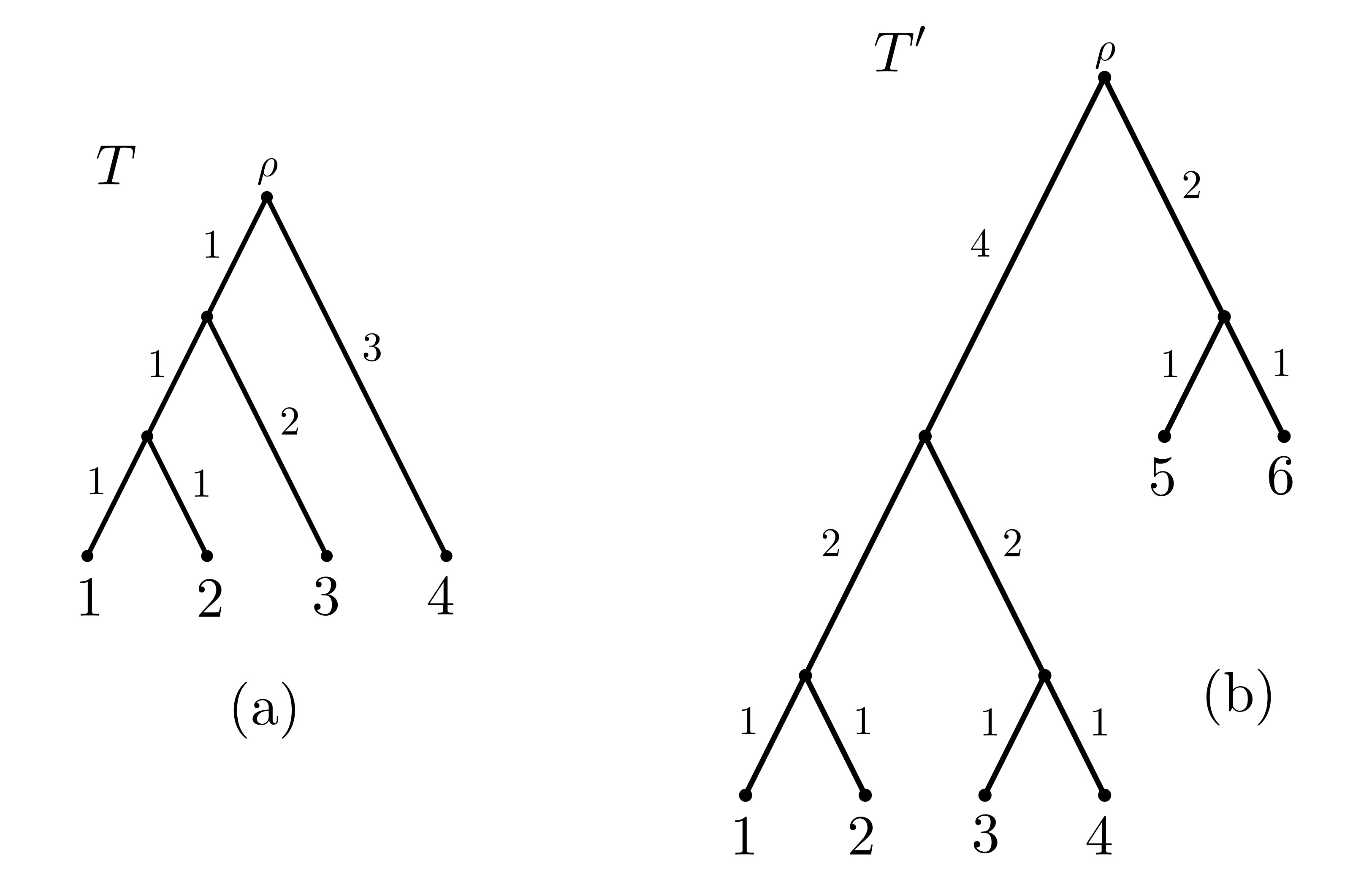 Figure 1
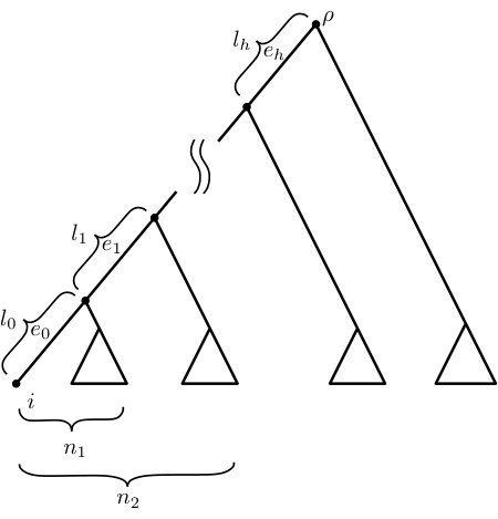 Figure 2
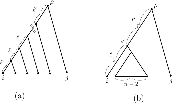 Figure 3
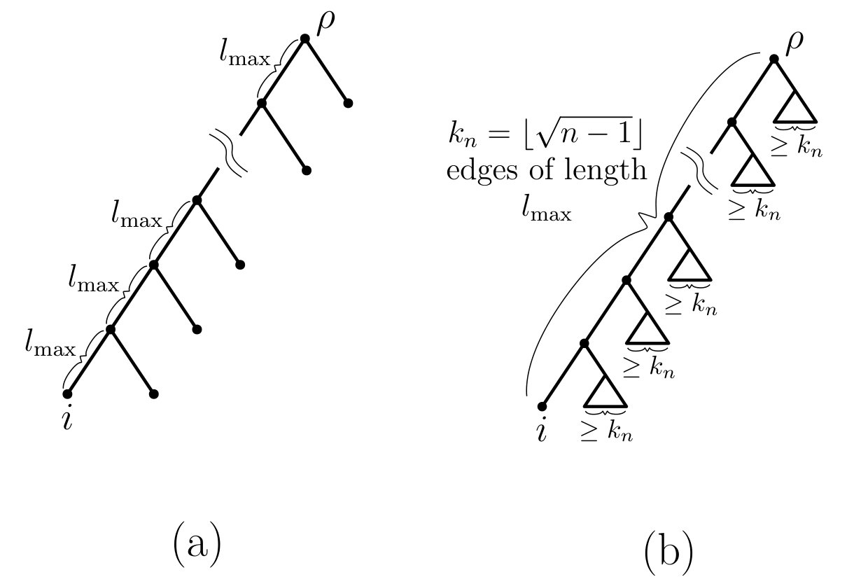 Figure 4
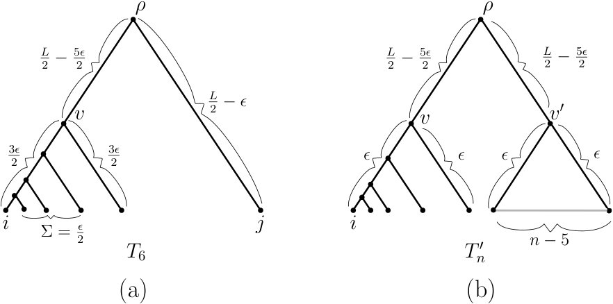 Figure 5
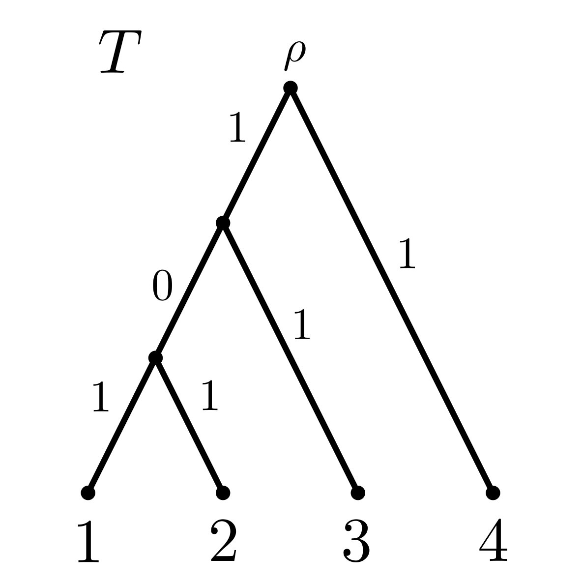 Figure 6
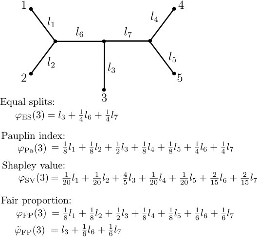 Figure 7
| pendant edge incident with | interior edge | pendant edge not incident with | |
|---|---|---|---|
Peer Reviews
No public reviews on file for this paper yet. If you reviewed it on a platform where reviews are public (OpenReview, ICLR, NeurIPS, ICML), you can paste yours below so the community can read it here.
Videos
No videos yet. Explain this paper in a talk, walkthrough, or lecture? Add one.
∎
11institutetext: K. Wicke 22institutetext: Institute of Mathematics and Computer Science, University of Greifswald, Germany. Orchid ID: 0000-0002-4275-5546 33institutetext: M. Steel 44institutetext: Biomathematics Research Centre, University of Canterbury, Christchurch, New Zealand (corresponding author). Orchid ID: 0000-0001-7015-4644
44email: [email protected]
Combinatorial properties of phylogenetic diversity indices
Kristina Wicke
Mike Steel
(Received: date / Accepted: date)
Abstract
Phylogenetic diversity indices provide a formal way to apportion ‘evolutionary heritage’ across species. Two natural diversity indices are Fair Proportion (FP) and Equal Splits (ES). FP is also called ‘evolutionary distinctiveness’ and, for rooted trees, is identical to the Shapley Value (SV), which arises from cooperative game theory. In this paper, we investigate the extent to which FP and ES can differ, characterise tree shapes on which the indices are identical, and study the equivalence of FP and SV and its implications in more detail. We also define and investigate analogues of these indices on unrooted trees (where SV was originally defined), including an index that is closely related to the Pauplin representation of phylogenetic diversity.
Keywords:
Phylogenetic tree, diversity index, Shapley value, biodiversity measures
††journal: Journal of Mathematical Biology
1 Introduction
Phylogenetic trees play an important role in quantifying biodiversity by estimating how much ‘evolutionary heritage’ is captured by each species and thus how much may be lost due to the current high rates of species extinction. The concept that each extant species caries a combination of unique and shared evolutionary history leads naturally to the notion of a phylogenetic diversity index for each species, which depends on its placement in the underlying phylogenetic tree, which, when summed together (across all species), gives the total diversity of the tree (Redding et al., 2008, 2014; Vellend et al., 2011). For example, the reptile species tuatara, being the sole surviving species from the superorder Lepidosauria, represents 220 million years of unique evolution as traced back to when this species branched off its phylogenetic tree from other lineages that have survived to the present. This species also carries further evolutionary history that is shared with other extant species, and phylogenetic diversity indices quantify not only the unique evolutionary history, but shared history as well.
Methods to apportion the total evolutionary history of life (measured in time or in genetic or trait diversity) across present-day species can be implemented in various ways. In this paper, we explore the mathematical relationship between three closely related indices. Two of these indices – (FP) Fair Proportion (Redding, 2003) and (ES) Equal Splits (Redding and Mooers, 2006) – were described for rooted trees, while a third, the Shapley Value (SV), from cooperative game theory, was initially introduced for unrooted trees (Haake et al., 2008). Soon afterwards it was shown that SV on rooted trees is actually equivalent to FP (Fuchs and Jin, 2015) (see also Stahn (2017)). These and other related indices, have been incorporated into the EDGE initiative by the Zoological Society of London (Isaac et al., 2007) to quantify the expected loss of evolutionary history associated with different endangered species.
The structure of this paper is as follows. We first review some basic definitions, then define two of the indices (FP and ES). Next, we consider how different FP and ES can be from each other. We do this first by considering their ratios (FP/ES and ES/FP) to obtain concise exact results (Theorem 2.1) which apply regardless of whether or not a molecular clock assumption is imposed. As a simple example of how these results apply, consider all rooted binary phylogenetic trees that classify (say) 20 species at their leaves and all possible assignments of edge lengths. It is then possible for the ES index of a species to be up to 9 times larger (but no more) than the FP index for that species; on the other hand, the FP index of a species can be up to 13,797 times larger (but no more) than the ES index of that species.
We then consider how large the differences FPES and ESFP can be, where now we need to bound some aspect of the tree length—either the longest edge length (Theorem 2.2) or the total length of the tree (Theorem 2.3). Companion results are also derived for molecular clock trees. In Theorem 3.1, we characterise the set of trees for which FP and ES are identical, and Section 4 provides a proof that SV is uniquely characterized by four axioms on trees, by using the equivalence of FP and SV. In Section 5, we consider variants of FP and ES defined on unrooted trees and establish a number of results for these measures. We end by highlighting some questions for future work.
1.1 Rooted trees and phylogenetic diversity indices
In this section and the next we deal with rooted phylogenetic –trees. A rooted tree with leaf set is said to be a (rooted) phylogenetic –tree if each non-leaf vertex is unlabelled and has out-degree at least 2 (two such trees are considered identical if there is a graph isomorphism between them that sends leaf to leaf for each ). In the case where all of the non-leaf vertices have out-degree 2, we say that the tree is binary; we will mostly work with this class in these two sections. Background on the basic combinatorics of phylogenetic trees can be found in Steel (2016). For the rest of this paper we will take, without loss of generality, the leaf set of trees to be , where .
Throughout this section, let be a rooted binary phylogenetic tree with root and leaf set , where each edge is assigned a non-negative length . Let be the total sum of edge lengths of (see Figure 1(a)).
Any function such that is called a phylogenetic diversity index or PD index for short. If can be written as a linear function on the edge lengths of , i.e.
[TABLE]
for coefficients that are independent of , we call a linear diversity index. In this paper, we will consider three linear PD indices, namely the Fair Proportion index, the Equal Splits index and the Shapley value. Note that an arbitrary function of the form described in Eqn. (1) is a diversity index if and only if the following linear equations hold for the coefficients , for each edge of :
[TABLE]
1.2 Fair Proportion and Equal Splits
The Fair Proportion (FP) index (Redding, 2003) for leaf (also called ‘evolutionary distinctiveness’) is defined as:
[TABLE]
where denotes the path in from the root to leaf , is the length of edge and is the number of leaves descended from . Essentially, the FP index distributes each edge length evenly among its descendant leaves. Note that as the order of summation in the definition of the FP index does not matter, we will often reverse the order and go from leaf to the root, since this is common biological practice. As an example, for the tree shown in Fig. 1(a) and the leaf , we have .
A second natural index is the Equal Splits (ES) index (Redding and Mooers, 2006), where each edge length is distributed evenly at each branching point. It is defined as:
[TABLE]
where if is a pendant edge incident with ; otherwise, if is an interior edge, then is the product of the out-degrees of the interior vertices on the directed path from to leaf . Since we will be dealing with binary trees in this paper, is 2 raised to the power of the number of edges between and leaf . As an example, for the tree shown in Fig. 1(a), and the leaf , we have (where we have again reversed the order of summation).
Both FP and ES are linear diversity indices (in particular, ). This is easy to see for FP but is less obvious for ES (it suffices to show that Eqn. (2) holds, which is given by Lemma 2 later in this paper). In general, , with Figure 1(a) providing a simple example. This raises the question of how different FP and ES can be, and under which circumstances they coincide. Although there have been some simulation studies to compare the two indices on various trees and taxon choices (Redding et al., 2008, 2014), in the first part of this paper, we determine the largest difference possible between one index and the other (both in relative terms and for absolute differences), and also considering the differences when the edge lengths are constrained to be ‘clock-like’ or not. In particular, rather than considering how different these indices might be ‘on average’ or for a particular tree with particular edge lengths, we study how different they can be for rooted trees in the most extreme cases.
2 How different can FP and ES be?
In this section, we investigate the maximal difference (across all binary trees with leaves and all edge lengths, and all leaf choices) between the Fair Proportion index and the Equal Splits index (and vice versa), both in terms of their ratios and their absolute values. Before proceeding, we introduce some further notation that will be helpful in the arguments that follow. Let , , denote the set of all binary rooted phylogenetic trees on leaf set .
Notice that each pair , where in , is a leaf of , gives rise to a uniquely defined directed path from the root of to leaf . We will let denote the number of leaves descended from the endpoint of closest to the leaves. Thus, and for all . In addition, when the edge has an associated non-negative length , we will let denote this length. We will use this notation throughout this paper. In the case where for all and (i.e. when each of the pendant subtrees in Fig. 2 has just one leaf), then is said to be a rooted caterpillar tree, with in its cherry (a cherry is a pair of leaves adjacent to the same vertex). Note that a tree in is a caterpillar if and only if it has exactly one cherry.
We will also occasionally consider a further ‘molecular clock’ condition on the edge lengths:
- (MC) The sum of the edge lengths from the tree root to leaf takes the same value for each leaf .
This condition applies, for example, if the edge lengths correspond to time, and all the leaves at the tree are sampled at the same time (e.g. at the present; cf. Figure 1(a)).
2.1 Maximal ratios
We first consider how large the FP can be relative to ES (i.e. as a ratio), as well as the ratio of ES to FP. Let
[TABLE]
and
[TABLE]
where (here and below) ‘sup’ refers to supremum (over all assignments of edge lengths that are positive).
In words, measures the largest possible ratio of the FP index to the ES index across all binary trees with leaves, all choices of leaf , and all assignments of strictly positive edge lengths. Similarly, measures the analogous extreme value for the ratio of ES to FP. Throughout this paper, we impose strictly positive edge lengths (in taking the supremum), in order to avoid any ambiguity as to whether an edge in a tree with a zero length edge should be contracted (this causes a discontinuity for the ES value), and to avoid any issues associated with fractions of the form .
Our first theorem shows that, in the most extreme case, the ratio of FP to ES grows exponentially with , whereas the ratio of ES to FP grows only linearly with .
Theorem 2.1
For :
[TABLE]
Moreover, these results hold if the molecular clock condition (MC) is imposed.
Proof
Our proof makes use of the following classical inequality, due to Cauchy (for details, see Steele (2004), pp. 82). Let be constants for . Then
[TABLE]
For the first ratio (FP/ES), using the notation in Fig. 2, we have:
[TABLE]
and since , we have:
[TABLE]
where the second inequality is from (5). Now, the expression on the far right of (6) is maximised (subject to the constraint that ) by taking , which gives:
[TABLE]
To see that this bound can be realised (in the supremum limit), consider a caterpillar tree that has leaf in its cherry and where the edges on the path from to have strictly positive edge lengths , respectively (see Fig. 3(a)). In the limit as the ratio tends to infinity, converges to which, combined with Inequality (7), establishes the first equality in Theorem 2.1. Moreover, it is clear that one can select the other edge lengths in so that the (MC) condition holds.
For the proof of the second equality in Theorem 2.1, we have:
[TABLE]
By Inequality (5), we have:
[TABLE]
Now, and for each we have . Subject to these constraints, the ratio is maximised by setting (with ). Thus
[TABLE]
To see that this bound can be realised, let be such that the children of the root consist of a leaf and an interior vertex , where the children of consist of leaf and a subtree of having leaves. Let the edge between the root and have length and assign length to the edge (see Fig. 3(b)). In the limit as the ratio tends to infinity converges to which, combined with Inequality (9), establishes the second part of Theorem 2.1. Again, it is clear that one can select the other edge lengths in so that the (MC) condition holds.
2.2 Maximal differences in terms of .
In this section and the next, we consider the additive difference between and and vice versa for any tree and any leaf of . These differences can be expressed as follows:
[TABLE]
Note that both sums start at , since for we have and so the additional term in either sum that would correspond to is zero. Also, in contrast to the ratios considered in the last section, these differences can be arbitrarily large (e.g. multiplying all the edge lengths by a constant will increase the difference by ). Thus we will analyse these maximal differences both in terms of the length of the longest edge of a tree and in terms of the sum of edge lengths .
Our second theorem shows how the absolute differences between FP and ES (and vice versa) grow either slowly (logarithmically) or are bounded independent of . In particular, the absolute difference between FP-ES can be made arbitrarily large (for a fixed value of ) by increasing the number of taxa; however, ESFP cannot (it is always bounded above by regardless of ). Moreover, if we impose a molecular clock, then FPES now becomes bounded above by a constant times . The situation with absolute differences is thus quite different from that for the ratios FP/ES and ES/FP.
To state the theorem more succinctly, we introduce some additional notation. Let
[TABLE]
In words, is the largest possible difference between FP and ES across the set of
- •
binary trees with leaves, and
- •
assignments of positive edge lengths to that have a maximal edge length , and
- •
choices of leaf .
Similarly, let
[TABLE]
Note that for . In the following theorem, we consider the case , and we let denote the Euler–Mascheroni constant (), and denote a term that converges to 0 as grows.
Theorem 2.2
For each :
- (i)
- (a)
.
- (b)
* *and **
[TABLE] 2. (ii)
If (MC) holds, then .
Proof of Part (i–a): We first show that a triple that realizes the quantity is a rooted caterpillar tree on leaves with being a leaf of the cherry in , and each edge on the path from the root of to having length . This is illustrated in Fig. 4(a). Let and be as described in Fig. 2. Let denote the contribution of edge to (cf. Eqn. (10)). Using only the fact that it follows that for each and so . In particular, , and so is maximal if and only if . As this holds for all values of , this immediately implies that the maximal pending subtree of containing leaf (call it ) has to be a caterpillar tree on leaves and with being a leaf of the cherry of this caterpillar. We show that (and thus is a caterpillar) by deriving a contradiction. Suppose that . In that case, the two subtrees of incident with the root of consist of and another subtree (call it ) that has two or more leaves. In particular, this implies that (i.e. there are less than edges on the path from to the root of ). However, as for each , this would imply that is not a tree that maximises , since could be increased by sequentially attaching all but one leaf from to the edge connecting and the root (i.e. by extending the length of the path from leaf to the root of ). Thus, , and therefore has to be the caterpillar tree on leaves that has in its cherry. Moreover, by again invoking the inequality (for all ) and recalling that , we can also conclude that for all (as otherwise and thus, could be increased). In summary, has the structure claimed.
It is now straightforward to calculate for the optimal choice of described above. We have:
[TABLE]
Consequently,
[TABLE]
which completes the proof of Part (i–a).
Proof of Part (i–b): From Eqn. (11), we have:
[TABLE]
Thus, To show that let be a tree in which the path from the root to leaf has edges, and each of the subtrees incident with the vertices of (except the final leaf vertex) has at least leaves. Assign edge length to each of the edges in . This is illustrated in Fig. 4(b). Then
[TABLE]
Now, and since , we have:
[TABLE]
as . Combining this with Eqn. (12) gives: , as required.
Proof of Part (ii): Let and . From Eqn. (10), we have We claim that, under condition (MC),
[TABLE]
To establish Inequality (13), the (MC) condition implies that for each leaf of descended from the endpoint of closest to the leaves, the sum of the edge lengths from to leaf is equal to . Moreover, each of these edges has length at most , which means that the number of edges on this path must be at least . Now, for , let be the number of vertices descended from that are separated from by exactly edges. We then have for all . This follows from an inductive argument. Clearly, (as is binary and is not a leaf since ). Suppose the statement is true for and consider . Each vertex counted by must have two children (otherwise there would be a leaf that is separated from by less than edges) and thus , which completes the inductive step. Now, as all leaves descended from are separated by at least edges from , we have , which completes the proof.
Thus, from Eqn. (13) and Eqn. (10), we have:
[TABLE]
To complete the proof of Part (ii), we require the following lemma, the proof of which is provided in the Appendix.
Lemma 1
Suppose that all lie in the interval . Then
[TABLE]
We apply this lemma by setting for . By Inequality (14), we have:
[TABLE]
as required, where the last inequality is from Lemma 1.
2.3 Maximal differences in terms of
We now describe the maximal possible (positive and negative) difference between FP and ES in terms of the total length of the tree (), rather than in terms of (this is summarized in Theorem 2.3 below). Let
[TABLE]
In words, is the largest possible difference between FP and ES across the set of:
- •
binary trees with leaves, and
- •
assignments of positive edge lengths to for which the total sum of the edge lengths is , and
- •
choices of leaf .
Similarly, let
[TABLE]
Theorem 2.3
**
- (i)
[TABLE]
where
[TABLE]
and for :
[TABLE]
- (ii)
If the molecular clock (MC) condition is imposed then the above expressions for and remain true if is replaced by .
Proof
For Part (i), we first show that for any given tree and any leaf of we have:
[TABLE]
Recall from Eqn. (10) that , and observe that for , we have . Thus, in particular, we have:
[TABLE]
Moreover, for any tree , we always have: for each , and therefore
[TABLE]
Let for . The sequence for begins as follows:
[TABLE]
after which the values in the sequence begin to decline. This establishes Inequality (15), as required.
To show that Inequality (15) is an equality, it suffices to show that for each and every there exists a tree with positive edge lengths and there is a leaf of for which . To this end, let be a rooted caterpillar tree with leaves, let be a leaf in the cherry of , let the interior edge at distance from leaf have length , and the lengths of all the remaining edges of have strictly positive lengths that sum to . In this case:
[TABLE]
holds for as required.
We turn now to . We first show that for any given tree and any leaf of :
[TABLE]
From Eqn. (11), we have: Now, takes a value that is, at most, for all . Thus:
[TABLE]
as required to establish Inequality (16).
To show that Inequality (16) is an equality it suffices to show that for each , and every there exists a tree with positive edge lengths, and there is a leaf of for which
[TABLE]
To this end, let be any tree for which the children of the root consist of a leaf and an interior vertex , where the children of consist of a leaf and a subtree of having leaves. Let the edge between the root and have length and let the remaining edges have strictly positive lengths that sum to . Then
[TABLE]
as required.
Part (ii): We now impose the (MC) condition. For , observe that our proof of Inequality (15) invoked the inequality . When (MC) holds, we have a tighter bound of the sum, namely since there is at least one other leaf of for which the path from the root of to also has length (by (MC)) and is edge-disjoint from the path from to (thus ). In this way, we claim that
[TABLE]
when (MC) holds.
To show that this inequality holds it suffices to show that for each , and every there exists a tree with positive edge lengths, and there is a leaf of for which:
[TABLE]
where is a term that tends to zero as . This trivially holds for (indeed it holds for ); while for let be a caterpillar tree with being a leaf in its cherry. Let and denote the two edges incident with the root of , where is a leaf. Assign the edge length and the edge length . We then assign the path from to and from to its adjacent leaf (which exists since it is a caterpillar) a length of . Now adjust the remaining edge lengths so they sum to and so that the (MC) condition holds for (see Fig. 5(a) for the case ). This assignment then satisfies Inequality (17) for , as required.
For the case , let be obtained from (in the previous argument) by replacing leaf by an arbitrary rooted binary subtree with leaves with root . Assign length to each of the two edges ( and ) that are incident with the root. Set the length of the path from to leaf , and the length of the path from to its adjacent leaf to equal , and set the length of each of two disjoint paths from to some pair of descendant leaves also equal to (see Fig. 5(b)). Finally, select edge lengths within these two subtrees so as to maintain the (MC) condition and so that the sum of the lengths of the additional edges added to these two subtrees is . In this way, the (MC) condition holds for the tree, equals the sum of the edge lengths, and Inequality (17) holds for , as required.
We now establish Part(ii) for the quantity . The argument for the inequality when (MC) holds is identical to the corresponding inequality for under (MC). Moreover, to show that this inequality can be realised, consider again the tree described in the previous paragraph, to which we will assign similar but modified edge lengths (we can assume that , since the equality holds when ). For the edge between the root and , assign length ; for the edge between the root and leaf , assign length ; for the edge assign length and assign the lengths of the remaining edges so that they sum to and are chosen so as to satisfy (MC) (this is possible, since we are assuming that ). In this way, the total sum of edge lengths is and the path length from the root to each leaf takes the same value (namely, ), and the result of Part (ii) for now follows.
3 For which tree shapes do FP and ES coincide?
In the following, we will analyse for which tree shapes FP and ES coincide. Therefore, recall that a rooted binary tree can be decomposed into its two maximal pending subtrees and rooted at the direct descendants of the root. We denote this by writing (note that the order of and is not important, thus ). Now, let be a binary tree with leaves, in which each leaf is separated from the root by a path of precisely edges. We call this (unique shape) tree the fully balanced tree of height and denote it by . Note that we have , i.e. both maximal pending subtrees of a fully balanced tree of height are fully balanced trees of height . Using the notation of Fig. 2 it is thus easy to see that for a leaf of and an edge on the path from the root of to leaf we always have: . It is now not difficult to show that FP and ES coincide (for all choices of reference leaf ) on any fully balanced tree. However, there are other tree shapes for which FP and ES coincide (e.g. the tree in Fig. 1(b)). Therefore, let be a rooted binary tree, whose two maximal pending subtrees and are both fully balanced trees of height and , respectively (where and are not necessarily identical), i.e. . We call such a tree a semi-balanced tree. Then,
Theorem 3.1
Let be a rooted binary phylogenetic tree on taxon set and non-negative edge lengths . Then, we have: for all and all assignments of positive edge lengths if and only if is a semi-balanced tree.
Proof
We first show that if is a semi-balanced tree (i.e. ) we have for all . Therefore, let and denote the two maximal pending subtrees of . Recall that
[TABLE]
As both sums just run over edges on the path from the root to leaf , and are independent of if and vice versa. Let be a leaf of . As is a fully balanced tree, we have for all , and thus, using Eqn. (10), we immediately have
[TABLE]
(i.e. ). Analogously, this holds for all leaves of , so for all .
Now suppose that for all . By way of contradiction assume that is not a semi-balanced tree, i.e. assume that at least one of the maximal pending subtrees of , say , is not a fully balanced tree. This implies that there exists an interior vertex in with the following two properties:
- (i)
For the subtree rooted at we have: , where and denote the number of leaves of and , respectively. 2. (ii)
is chosen so that is a minimal subtree of satisfying property (i) (in the sense that there exists no subtree of on fewer leaves that has this property).
In particular, this implies that both maximal pending subtrees of are fully balanced trees. Without loss of generality we may assume that (otherwise exchange the roles of and ), in which case .
Now, for a leaf and an edge of , we use and to denote the contribution of edge to , respectively , where
[TABLE]
Let and . Now, as both maximal pending subtrees of are fully balanced trees, we can use the first part of the proof to conclude that for each : and we denote this common value by .
Now, let be the lengths of the edges on the path from vertex to the root and let be the number of leaves descended from edge . Let be a leaf of and let be a leaf of . By assumption, for all , and so we have
[TABLE]
In particular
[TABLE]
However, as and for all , this is a contradiction. A similar argument yields a contradiction for the assumption that is not a fully balanced tree. Thus, has to be a semi-balanced tree, which completes the proof.
4 Uniqueness of SV for phylogenetic tree games
Another linear PD index frequently used is the so-called Shapley value (SV), which originates from cooperative game theory. Recall that a cooperative game is a pair consisting of a set of players and a characteristic function that assigns a real value to all subsets of with . A function that assigns a payoff to each player is called a value for the game. One such value is the Shapley value (Shapley (1953)), which is defined as follows:
[TABLE]
Note that the Shapley value of a player reflects the average marginal contribution of to the game. Moreover, it is characterised by the following four axioms:
Pareto efficiency: . 2. 2.
Symmetry: with and , if , then . 3. 3.
Dummy axiom: If , , then . 4. 4.
Additivity:
In fact, the Shapley value is the unique value satisfying these four axioms.
Theorem 4.1
The Shapley value is the unique value satisfying Axioms 1–4 (Shapley (1953); Winter (2002)).
Note that the formulation described here is slightly different from the original formulation in Shapley (1953). On the one hand, Shapley (1953) used a framework consisting of three axioms: symmetry, additivity, and a carrier axiom, the latter comprising both Pareto efficiency and the dummy axiom (see Winter (2002) for details). On the other hand, Shapley (1953) made the additional assumption that is a superadditive function (i.e. for all pairs of disjoint sets ), which was later relaxed by Dubey (1975).
In the phylogenetic setting, is taken to be the phylogenetic diversity of on 111Note that PD is not a superadditive function. In fact, it is submodular, satisfying the property that for all (cf. Proposition 6.13 in Steel (2016))., denoted by PD_{{\color[rgb]{0,0,0}T}}(S), and defined as the sum of lengths of the edges in the minimal subtree of that contains and the root of (cf. Faith (1992)). As an example, for the tree depicted in Fig. 1(b), and the subset of leaves, we have PD_{{\color[rgb]{0,0,0}T^{\prime}}}(S)=11.
Considering the leaf set of a rooted phylogenetic tree as the set of players and phylogenetic diversity as the characteristic function of a game, Eqn. (18) becomes:
[TABLE]
Note that in contrast to the previous two sections we are not assuming in this section that is a binary tree.
In an important paper, Fuchs and Jin (2015) proved that the Shapley value and the Fair Proportion index on rooted phylogenetic trees agree (see also Steel (2016) and Stahn (2017)).
Theorem 4.2 (Fuchs and Jin (2015))
The Fair Proportion index and the Shapley value are identical on rooted phylogenetic trees, i.e. for all :
[TABLE]
In the following we will use this result to show that SV is the unique value satisfying Axioms 1–4 for the sub-class of games induced by a rooted tree and the phylogenetic diversity function. This is not obvious since (as noted by Haake et al. (2008) in the setting of PD on unrooted trees), the class of games based on PD on a rooted tree is smaller than the class of all games (for which Theorem 4.1 states that SV is unique). Apart from SV there might be other functions that satisfy these 4 axioms for this smaller class of games, and so SV might not be uniquely determined by them. In Theorem 4.3, however, we show that SV is still uniquely characterised by the 4 axioms for this smaller class of games. Haake et al. (2008), by contrast, introduced an additional axiom to obtain their characterization (Theorem 9 of that paper).
Let denote the class of games induced by a rooted phylogenetic tree with leaf set and non-negative edge lengths, and the phylogenetic diversity function on . Moreover, let a pair denote a PD game. Note that such a pair can be represented as a linear combination of so-called basis games (for ), where corresponds to the game on tree , in which edge has length 1 and all other edges have length 0. It can be shown that the family {\color[rgb]{0,0,0}(PD_{T_{e}})}_{e\in E(T)} is linearly independent and forms a basis of of dimension .
The following theorem provides an axiomatic characterization of SV for games in .
Theorem 4.3
There is a unique function
[TABLE]
that satisfies Axioms 1–4. This function coincides with the Shapley value, i.e. {\color[rgb]{0,0,0}\psi_{PD_{T}}}(i)=SV_{T}(i) for all .
Proof
By Theorem 4.1, SV satisfies Axioms 1–4.
Now, let be a PD game and let {\color[rgb]{0,0,0}\psi_{PD_{T}}} satisfy all Axioms 1–4. We first consider a basis game and determine {\color[rgb]{0,0,0}\psi_{PD_{T_{e}}}}.
Let denote the set of leaves descended from and let . Then, all leaves not in are dummy players, as for all , we have that for all . As satisfies the dummy axiom, this implies that for all . On the other hand, all leaves in are symmetric players as for any pair (with ), we have that PD_{{\color[rgb]{0,0,0}T_{e}}}(C\cup\{i\})=PD_{{\color[rgb]{0,0,0}T_{e}}}(C\cup\{j\})=1 holds for all subsets of . As this holds for all pairs and as \psi_{{\color[rgb]{0,0,0}PD_{T_{e}}}} satisfies symmetry, we can conclude that \psi_{{\color[rgb]{0,0,0}PD_{T_{e}}}}(i)=\psi_{{\color[rgb]{0,0,0}PD_{T_{e}}}}(j) for all . On the other hand, since \psi_{{\color[rgb]{0,0,0}PD_{T_{e}}}} satisfies efficiency, we have
[TABLE]
which – using symmetry – implies that \psi_{{\color[rgb]{0,0,0}PD_{T_{e}}}}(i)=\frac{1}{n(e)} for all . To summarize, \psi_{{\color[rgb]{0,0,0}PD_{T_{e}}}}(i)=\frac{1}{n(e)} for all and \psi_{{\color[rgb]{0,0,0}PD_{T_{e}}}}(j)=0 for all . It is easily verified that these values coincide with the FP index and thus with the SV (by Theorem 4.2).
Analogously, one can show that is a linear function. As satisfies Axiom 4, it is additive. Moreover, for all , let denote the PD game on tree , in which edge has length and all other edges have length 0. Then, using the same notation and reasoning as above, we have for all , , and for all , . Comparing this with from above, it is now easy to see that we have for all and all .
Together with the additivity of and SV this implies that coincides with SV for all games in .
Remark 1
Since SV is the unique index satisfying Pareto efficiency, symmetry, the dummy axiom and additivity for the class of games induced by a rooted tree and PD (by Theorem 4.3), and since SV and FP agree for rooted trees (by Theorem 4.2) and, in general, ES FP, it follows that ES must violate at least one of these four axioms. It can easily be checked that ES satisfies Pareto efficiency, additivity and the dummy axiom, but it may violate symmetry. An example is given in Figure 6, where we have , even though PD_{{\color[rgb]{0,0,0}T}}(C\cup\{1\})=PD_{{\color[rgb]{0,0,0}T}}(C\cup\{3\}) for all (on the other hand, ).
5 Diversity indices for unrooted trees
We now consider phylogenetic diversity indices for unrooted trees. An unrooted tree with leaf set is said to be an unrooted phylogenetic –tree if each non-leaf vertex is unlabelled and has degree at least 3 (two such trees are considered equivalent if there is a graph isomorphism between them that sends leaf to leaf for each ). In the case where all non-leaf vertices in have degree exactly equal to 3, is said to be binary. Background on the basic combinatorics of unrooted phylogenetic trees can be found in Steel (2016).
Let be an unrooted phylogenetic tree (not necessarily binary) with leaf set and let all edges have non-negative edge lengths . For a subset of the leaves, the (unrooted) phylogenetic diversity of is defined as the sum of the edge lengths of the minimal subtree connecting the leaves in . Note that PD_{{\color[rgb]{0,0,0}T}}(\{i\})=0 for all and PD_{{\color[rgb]{0,0,0}T}}([n]) is the total sum of edge lengths of (i.e ). For a leaf and an edge of , let be the set of interior vertices of in the path in from to edge (including the first vertex of that is reached, but not the second), and for each vertex of let denote the degree of . For each edge of , let
[TABLE]
where we adopt the convention that if (i.e. is a pendant edge incident with leaf ) then and hence .
5.1 Unrooted Equal Splits
In this section, we develop a version of Equal Splits for unrooted trees. Recall that for rooted trees, the definition of the ES index is , where if is a pendant edge incident with ; otherwise, if is an interior edge, then is the product of the out-degrees of the interior vertices on the directed path from to leaf .
This definition does not directly apply to unrooted trees, since there is no reference root vertex in an unrooted tree. Moreover, introducing a phantom root vertex in an unrooted tree results in different ES index values, depending on where the phantom root is inserted. Nevertheless, we can define a canonical unrooted version of ES that is a diversity index as follows.
Let
[TABLE]
where the summation is over all edges of and where
[TABLE]
Note that is the expression introduced in Eqn. (19). Moreover, note that in contrast to the rooted setting, is defined as a sum over all edges of and not only over edges on a certain path in . In fact, even though pendant edges not incident with leaf do not contribute to (since in that case), the edges that do contribute do not necessarily form a path in (cf. Fig. 7).
Theorem 5.1
For any unrooted phylogenetic tree , is a diversity index for . In other words:
[TABLE]
In order to prove this theorem, we require the following technical lemmas:
Lemma 2
Suppose that is a rooted phylogenetic tree with leaf set and root vertex . Let denote the out-degree of vertex . We then have:
[TABLE]
Proof
We use a simple probabilistic argument. Consider a random walk, starting from the root vertex and proceeding towards the leaves. At each interior vertex , one of the child vertices of is chosen uniformly at random (and independently of earlier choices). In this way, the probability of arriving at leaf is simply . Since we always arrive at one (and only one) leaf of by this process, , as required.
Corollary 1
Let be an unrooted phylogenetic tree with leaf set and let be an arbitrary edge of . Let and denote the subsets of leaves of that lie on each side of , with being closer to (if is a leaf, then ) and being closer to (again, if is a leaf, then ). In this case:
[TABLE]
Proof
Clearly, we only have to prove the first statement, so consider . If (which implies ), , and we again adopt the convention that in this case . In particular, the claimed statement holds for . Next, consider . Then the expression
[TABLE]
can also be written as:
[TABLE]
where is the rooted phylogenetic tree on leaf set and root vertex obtained from by deleting edge and the subtree of with leaf set . The corollary now follows from Lemma 2 by taking as the tree in that lemma, and . Note that the statement can alternatively be shown without the use of Lemma 2 by using an inductive argument.
Lemma 3
Suppose that the linear equation
[TABLE]
with , holds for all choices of of the form where and
[TABLE]
Eqn. (22) then holds for all choices of .
Proof
The proof involves simple linear algebra. Let . Eqn. (22) can then be rewritten as . Suppose this equation holds whenever (and for each choice of ). Then this equation becomes , and since this holds for all choices of , all the –coefficients are zero, which gives the result.
We are now in the position to prove Theorem 5.1.
Proof of Theorem 5.1: By Lemma 3, it suffices to establish Eqn. (20) when assigns length 1 to an arbitrary edge and 0 to all other edges. Then PD_{{\color[rgb]{0,0,0}T}}([n])=1 and the left hand side of Eqn. (20) is . Our aim then is to show that this last quantity is always equal to . This is true by definition of when is a pendant edge, so we may suppose that is an interior edge. In that case, let and denote the subsets of leaves of that lie on each side of , with being closer to than and being closer to than (thus , and ). Since (since is an interior edge) we have:
[TABLE]
and
[TABLE]
where the last equality follows from Corollary 1. A similar argument shows that , and so, by Eqn. (23), we obtain the required equality:
[TABLE]
5.2 A diversity index related to the Pauplin representation of phylogenetic diversity
PD_{{\color[rgb]{0,0,0}T}}([n]) can also be expressed as a positive linear combination of the pairwise distances between leaves and in various ways, one of them being the following representation described by Semple and Steel (2004):
[TABLE]
where
[TABLE]
and where denotes the set of interior vertices on the path from to in .
Although this representation holds for general trees (not only binary ones), for binary trees, this expression is also known as the Pauplin representation of phylogenetic diversity (cf. Pauplin (2000)). In the following section, we will further analyse this representation and suggest that it leads to yet another possible unrooted PD index. Let
[TABLE]
where the summation is over all edges of and is the expression introduced in Eqn. (19).
Theorem 5.2
Let be an unrooted phylogenetic tree with leaf set and let be a leaf of . In that case:
[TABLE]
In other words, is closely related to the Pauplin representation of PD given in Eqn. (24). Moreover, is a diversity index (i.e. \sum_{i\in[n]}\varphi_{\rm Pa}(i)=PD_{{\color[rgb]{0,0,0}T}}([n])).
Proof
Let be a leaf of . By Lemma 3 it suffices to establish Eqn. (25) when assigns length 1 to an arbitrary edge and 0 to all other edges. Note that the removal of edge splits into two subtrees. Let (=‘close’) denote the leaf set of the subtree that contains leaf and let (=‘far’) denote the leaf set of the other subtree. Now, for all leaves we clearly have:
[TABLE]
Thus, we have for the right-hand side of Equation (25)
[TABLE]
As lies on the path from to , the term on the right of this last equation can also be written as:
[TABLE]
where the last equality follows from applying Corollary 1. On the other hand, for the left-hand side of Equation (25), we have:
[TABLE]
as edge has length 1, while all other edges have length 0, which completes the proof of Eqn. (25). The claim that is a diversity index is now a direct consequence from Eqn. (24).
5.3 Unrooted Fair Proportion
Similar to the Equal Splits index, the Fair Proportion index has so far only been considered for rooted trees. In the following, we suggest two canonical extensions of Fair Proportion to unrooted trees. Recall that for rooted trees, the definition of FP is , where is the number of leaves descended from . Note that the removal of edge splits into two connected components and is the number of leaves of in the connected component that contains . This concept can be extended to unrooted trees as follows.
For a leaf and an edge of , let denote the size of the set of leaves that lie on the same side of as . Let
[TABLE]
and let
[TABLE]
where the summation is over all edges of and where
[TABLE]
Theorem 5.3
For any unrooted phylogenetic tree , and are diversity indices for . In other words,
[TABLE]
Proof
We first establish Eqn. (26). By Lemma 3, it suffices to establish Eqn. (26) when assigns length 1 to an arbitrary edge and 0 to all other edges. Then, PD_{{\color[rgb]{0,0,0}T}}([n])=1 and the left hand side of Eqn. (26) is . Now, let and denote the subsets of leaves that lie on each side of (i.e. , and ), in which case:
[TABLE]
Eqn. (27) follows from a similar argument by noting that the left hand side of this equation becomes . If is a pendant edge, this quantity is equal to 1 by definition of and if is an interior edge, the same reasoning as in the proof of Eqn. (26) establishes \sum_{i\in[n]}\mu_{\rm FP}(i,e^{\prime})=1=PD_{{\color[rgb]{0,0,0}T}}([n]).
5.4 Summary of unrooted diversity indices
In the last sections we have presented canonical extensions of Equal Splits and Fair Proportion to unrooted trees and have also introduced a diversity index closely related to the Pauplin representation of phylogenetic diversity. Although all these indices appear to be new, an unrooted Shapley value has long been known in the literature. In fact, even though the Shapley value is frequently used for rooted trees, it was first defined and introduced for unrooted trees by Haake et al. (2008) and can be expressed as follows:
[TABLE]
where the summation is over all edges of , is again the number of leaves that lie on the same side of as leaf , and is the number of leaves that lie on the other side of (cf. Theorem 4 in Haake et al. (2008)). Recall that for rooted trees, FP and SV are equivalent, so one might argue that the unrooted SV can be considered an unrooted analogue of FP. It turns out, however, that there exists a natural extension of FP to unrooted trees, that is different from unrooted SV.
In fact, although all of the unrooted diversity indices discussed above can be expressed as linear functions of the edge lengths of with coefficients that are independent of , these coefficients differ among indices (cf. Table 1) and the indices are, in general, not equivalent (cf. Figure 7).
6 Concluding Remarks
Phylogenetic diversity indices play a key role in biodiversity, so it is helpful to understand how the different indices are related. In this paper, we asked just how different they can be for rooted trees (in an extreme sense, rather than on average). We also considered how some of the natural indices in the rooted settings extend to the unrooted setting, and further explored the way in which the Shapley value relates to rooted and unrooted indices. Our work suggests two broad questions that may be interesting to explore in future work. First, how do the results in Sections 2 and 3 extend if we lift the assumption that the underlying trees are binary? Second, for the unrooted indices in Section 5, how different can they be from one another (in the sense we considered in Section 2) and for which trees are certain indices identical (in the sense we considered in Section 3)? Moreover, as all unrooted indices apart from the unrooted SV appear to be new, it additionally might be of interest to analyse their biological interpretation and relevance for conservation decisions.
7 Acknowledgements
We thank Arne Mooers for a number of helpful suggestions, and the two anonymous reviewers for detailed comments on an earlier version of this manuscript. We also thank François Bienvenu for pointing out an alternative proof of Lemma 1, and Mareike Fischer for helpful comments concerning Section 4. The first author also thanks the German Academic Scholarship Foundation for a doctoral scholarship.
Appendix: Proof of Lemma 1
Proof of Lemma 1: We first establish the following identity by application of the ‘fundamental theorem of calculus’. Let be any continuous function and let . We then have:
[TABLE]
To establish (28), let . Since is continuous, , so the left-hand side of Eqn. (28) can be written as which gives Eqn. (28).
Now, for all , , since takes values in the interval , and thus (28) gives:
[TABLE]
Taking in this last inequality gives:
[TABLE]
Let be a piecewise continuous function that takes the value on the open interval , for each , and let , be a sequence of continuous functions that converges in the norm to (e.g. by Fourier series). As , then converges to and converges to . Inequality (29) now establishes the lemma.
The reference list from the paper itself. Each links out to its DOI / PubMed record.
- 1Dubey (1975) Dubey, P., 1975. On the uniqueness of the Shapley value. International Journal of Game Theory 4, 131–139. URL: https://doi.org/10.1007/BF 01780630 , doi: 10.1007/BF 01780630 .
- 2Faith (1992) Faith, D.P., 1992. Conservation evaluation and phylogenetic diversity. Biological Conservation 61, 1–10. URL: http://dx.doi.org/10.1016/0006-3207(92)91201-3 , doi: 10.1016/0006-3207(92)91201-3 .
- 3Fuchs and Jin (2015) Fuchs, M., Jin, E.Y., 2015. Equality of Shapley value and fair proportion index in phylogenetic trees. Journal of Mathematical Biology 71, 1133–1147.
- 4Haake et al. (2008) Haake, C.J., Kashiwada, A., Su, F.E., 2008. The Shapley value of phylogenetic trees. Journal of Mathematical Biology 56, 479–497. URL: http://dx.doi.org/10.1007/s 00285-007-0126-2 , doi: 10.1007/s 00285-007-0126-2 .
- 5Isaac et al. (2007) Isaac, N., Turvey, S.T., Collen, B., Waterman, C., Baillie, J., 2007. Mammals on the EDGE: Conservation priorities based on threat and phylogeny. P Lo S One 2, e 296.
- 6Pauplin (2000) Pauplin, Y., 2000. Direct calculation of a tree length using a distance matrix. Journal of Molecular Evolution 51, 41–47. doi: 10.1007/s 002390010065 .
- 7Redding (2003) Redding, D.W., 2003. Incorporating genetic distinctness and reserve occupancy into a conservation priorisation approach. Master’s thesis. University Of East Anglia, Norwich, UK.
- 8Redding et al. (2008) Redding, D.W., Hartmann, K., Mimoto, A., Bokal, D., De Vos, M., Mooers, A.Ø., 2008. Evolutionarily distinctive species often capture more phylogenetic diversity than expected. Journal of Theoretical Biology 251, 606–615. doi: 10.1016/j.jtbi.2007.12.006 .