A note on Sobolev type inequalities on graphs with polynomial volume growth
Li Chen

TL;DR
This paper establishes generalized Sobolev and Poincaré inequalities on graphs with polynomial volume growth, demonstrating their optimality on Vicsek graphs, thus advancing the understanding of functional inequalities in discrete geometric settings.
Contribution
It introduces a scale of optimal Sobolev and Poincaré inequalities on graphs with polynomial volume growth, including Vicsek graphs.
Findings
Proved generalized $L^p$-Poincaré inequalities.
Established Sobolev type inequalities on specific graphs.
Demonstrated optimality of inequalities on Vicsek graphs.
Abstract
We prove a scale of generalized -Poincar\'e inequalities and Sobolev type inequalities on graphs with polynomial volume growth. They are optimal on Vicsek graphs.
Click any figure to enlarge with its caption.
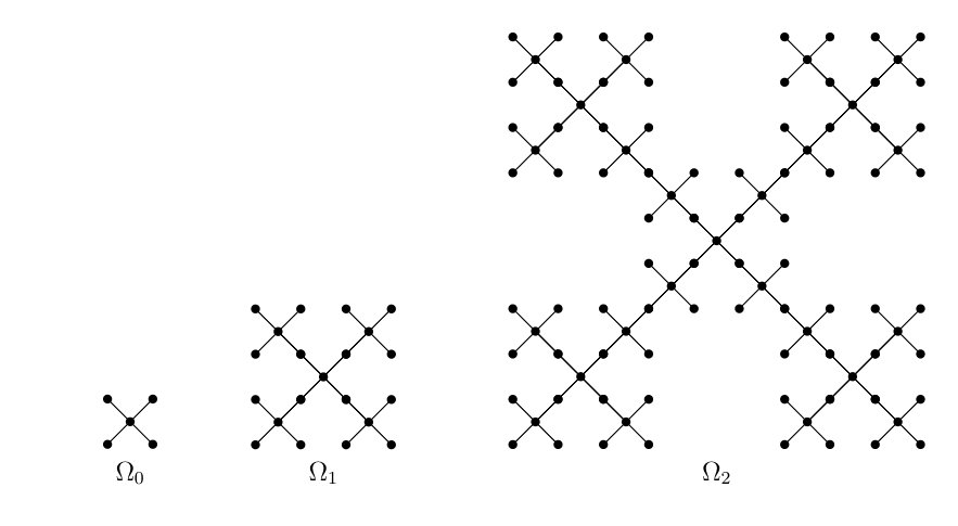 Figure 1
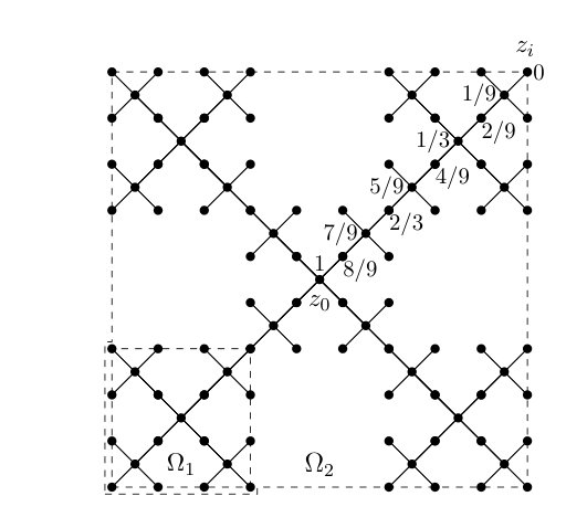 Figure 2
Peer Reviews
No public reviews on file for this paper yet. If you reviewed it on a platform where reviews are public (OpenReview, ICLR, NeurIPS, ICML), you can paste yours below so the community can read it here.
Videos
No videos yet. Explain this paper in a talk, walkthrough, or lecture? Add one.
Taxonomy
TopicsGeometric Analysis and Curvature Flows · Geometry and complex manifolds · Nonlinear Partial Differential Equations
A note on Sobolev type inequalities on graphs with polynomial volume growth
Li Chen
Department of Mathematics, University of Connecticut, Storrs, CT 06269
Abstract.
We prove the generalized -Poincaré inequalities and Sobolev type inequalities on graphs with polynomial volume growth. They are optimal on Vicsek graphs.
1. Introduction
The classical Sobolev inequalities play a crucial role in analysis and partial differential equations in Euclidean spaces. In many different settings, Sobolev inequalities have been deeply explored and they are extremely flexible and useful. For a nice introduction of previous work, we refer to the survey by L. Saloff-Coste [15], see also the comprehensive book [14].
In this note we work on a scale of Sobolev type inequalities of great generality in the setting of graphs, which was first introduced by T. Coulhon in [7] on manifolds and graphs. Let and , consider on an infinite graph the following scale of inequalities
[TABLE]
for any finite subset of and any function supported in , where denotes the measure of .
The above inequalities are also quoted as Faber-Krahn type inequality (see for instance [7, page 88]). When , the inequality (1.1) is equivalent to the graph analogue of classical Sobolev inequalities. For more interpretations from either geometric or analytic aspects, we refer to [7, 6, 4]. Of the same spirit, a more general version of (1.1) was also studied in the context of manifolds and graphs in [6, 8, 10], that is,
[TABLE]
where is a non-decreasing function on to itself.
Volume lower bounds are important implications of the above two scales. Indeed, (1.1) implies that . For the more general scale, if is unbounded, then (1.2) for is equivalent to , where is the reverse function of (see [8, Proposition 2.2] or [6]). The reverse implication is well studied under the assumption of pseudo-Poincaré inequality
[TABLE]
where , where is the measure on . In fact, this allows the scale to go down from to , see [8, Proposition 2.6]. Compared with the Poincaré inequality
[TABLE]
the pseudo-Poincaré inequality may hold for more general situations, for instance on all unimodular Lie groups (see [8]). As is well-known, the Poincaré inequality and the volume doubling property imply the pseudo-Poincaré inequality (see for example [13], [14]). On graphs both the Poincaré and pseudo-Poincaré inequalities are very restrictive properties. However, under assumptions of volume growth, one can obtain analogues of the and -Poincaré inequalities, see [11, Section 5].
In this note, our goals are to generalize the results in [11] to the case on graphs with polynomial volume growth and hence to study the scale of Sobolev type inequalities in form of (1.2). We are particularly interested in explicit examples of Vicsek graphs (see [2, 3]).
In the following we introduce the setting of graphs, mainly following the notation in [4]. Let be a connected undirected infinite graph with the set of vertices and the set of edges . Endow with a symmetric weight , such that . We say that and are neighbors, i.e., , denoted by , if and only if .
Define , then it extends to a measure on by
[TABLE]
where is a finite subset in .
For , a path of length between and is a sequence with and . The induced graph distance is the minimal number of edges in any path connecting and . The graph is connected if for all . Define balls in by
[TABLE]
Any weighted graph admits a random walk on defined by the transition probabilities if and otherwise [math]. Then is a reversible Markov kernel satisfying
[TABLE]
Denote by and by the set of functions in with finite support. For , the norm of a function is given by
[TABLE]
The linear operator associated with the kernel is defined by
[TABLE]
We call the operator the (probabilistic) Laplacian on .
The value of the discrete gradient on is defined by
[TABLE]
Then we have that , where denotes the inner product on .
Throughout this paper, we always assume that
- •
is locally finite, i.e., there exists such that any has at most neighbors;
- •
and has controlled weights, i.e., there exists such that for all
[TABLE]
- •
The volume growth of is uniformly polynomial. That is, there exists such that .
Note that under these assumptions, we have that and for ,
[TABLE]
see, for example, [1, p. 313] for a proof.
Our main results are as follows.
Theorem 1.1**.**
Let be a locally uniformly finite weighted graph with controlled weight. Assume that . Then for , it holds that
[TABLE]
Theorem 1.2**.**
Let be a locally uniformly finite weighted graph with controlled weight and let be a bounded subset. Assume that . Then for , it holds
[TABLE]
Note that when , the above inequality () is trivial since it is equivalent to following the co-area formula (see for instance [8, Proposition 2.3]).
Define the escape time to be the mean exit time of a simple random walk on starting at from the ball with center and radius . We say has escape time exponent if for . Well known estimates for random walks on graphs imply that and . In particular, Vicsek graphs are borderline examples with (see [3]), which are of particular interest to us. In fact, we have
Proposition 1.3**.**
Let be a Vicsek graph. Then the Poincaré inequality () and Sobolev type inequality () in Theorems 1.1 and 1.2 are optimal for .
Remark 1.4**.**
In Theorem 1.1 and Theorem 1.2, we have variant parameters in inequalities () and (), which depends on and . When these inequalities are optimal, then the related parameters can’t be improved to smaller numbers.
The paper is organized as follows. In Section 2, we give the proof of Theorem 1.1. Section 3 provides two different proofs of Theorem 1.2. Finally, we study the special case of Vicsek graphs and prove Proposition 1.3.
2. Poincaré type inequalities
In this section, we will prove Theorem 1.1. Recall that under assumptions of volume growth, the and -Poincaré type inequalities were partially obtained in [11]. In fact, if the the volume growth is uniformly polynomial, i.e., , then for any ,
[TABLE]
and
[TABLE]
We will extend ideas from [11] (see also [12]) to prove our first result.
Proof of Theorem 1.1.
For any , we choose as one of the shortest paths from to . Define . Let be an oriented edge in a path from to and .
Since
[TABLE]
for , we have
[TABLE]
In the last inequality, depends on the weight .
For , the Hölder inequality leads to
[TABLE]
Since has controlled weights, the last term is bounded from above by
[TABLE]
Take for , then we get from (1.6)
[TABLE]
One can see that . Therefore,
[TABLE]
Since , we have
[TABLE]
This leads to () and hence we finish the proof. ∎
The pseudo-Poincaré type inequality follows now as a corollary.
Corollary 2.1**.**
Let be a locally uniformly finite weighted graph with controlled weight. Assume that . Then for , it holds that
[TABLE]
The proof is the similar to the one that Poincaré inequality together with the volume doubling property implies the pseudo-Poincaré inequality, see for instance [14, Lemma 5.3.2]. We leave details to the interested reader.
3. Sobolev type inequalities
In this section, we will prove Theorem 1.2, for which we provide two different approaches. One is to use the Poincaré type inequality (), following [6, Section III] (see also [8, Proposition 2.6]).
Proof of Theorem 1.2.
We first treat the case . Note that for any in , there holds for any and
[TABLE]
Write
[TABLE]
It follows from Hölder inequalities, (), and (3.1) that
[TABLE]
Choosing to be the integer such that , then
[TABLE]
The inequality also holds for any .
Next let . For any , write
[TABLE]
Taking to be the integer such that . Therefore by ,
[TABLE]
Taking and yields , which is equivalent to . ∎
The second approach, without using the Poincaré inequality, is inspired by the Faber-Krahn inequality in [2]. That is, for a graph with controlled weights, the Faber-Krahn inequality as follows holds for any non-empty finite set ,
[TABLE]
where
[TABLE]
If has polynomial volume upper bound , the Faber-Krahn inequality is also the -Sobolev type inequality in our theorme. Moreover, this inequality is sharp at all scales of the volume on Vicsek graphs ([2, Theorem 4.1]).
An alternative proof of Theorem 1.2.
For any function , assume (otherwise we can normalize ). Then we have
[TABLE]
Consider a point such that and the largest integer such that the ball . Obviously we have . Also, there exists a sequence of points
[TABLE]
starting from and terminating at a point .
Therefore, by (1.6) and the Hölder inequality
[TABLE]
where the last inequality is due to the fact that
[TABLE]
It follows from (3.2) and (3.3) that
[TABLE]
Eventually, we obtain () and the proof is completed.
∎
4. Optimality on Vicsek graphs
Considering the Vicsek graphs, we assume that the weight is the standard weight. Recall the construction of a Vicsek graph on (taken from [9]): Let denote the cube in
[TABLE]
Construct an increasing sequence of finite graphs as subsets of . Let be the set of points containing all vertices of and the center of . Define edges in as segments connecting the center with the corners. Assuming that is already constructed, define as follows. The cube is naturally divided into congruent copies of ; select of the copies of by taking the corner cubes and the center one. In each of the selected copies of construct a congruent copy of graph , and define as the union of all copies of (merged at the corners). Then the Vicsek tree is the union of all , (see Figure 1).
Consider the natural weight if and otherwise [math]. For all , and , satisfies
[TABLE]
and
[TABLE]
where . By Theorem 1.1, the Vicsek graph satisfies the following scale-invariant Poincaré inequality: for any ,
[TABLE]
Since , this inequality is strictly weaker than ().
Proof of Proposition 1.3.
It suffices to show the optimality of the generalized Sobolev inequality () for . Indeed, note that we can obtain () from () in the proof of Theorem 1.2. If the exponent of in () is not optimal, then () can also be improved, which contradicts its optimality.
In fact, with the same functions and subsets, we can also show the optimality of () for .
Let be the same subset as in [2], where . Hence . Denote by the centre of and by its corners. Define as follows: , and extend as a harmonic function in the rest of . Then is linear on each of the paths of length , which connects with the corners , and is constant elsewhere. More exactly, if belongs to some , then . If not, then , where is the nearest vertex in certain line of and . See Figure 2, which we take from [2].
For any in the block with centre , we have . Therefore
[TABLE]
Also, since for any two neighbours on each of the diagonals connecting and , and otherwise , we obtain
[TABLE]
Finally combining the above two estimates, we have
[TABLE]
This finishes the proof. ∎
Remark 4.1**.**
In [5], it was proved that doesn’t hold for and hence by duality the Riesz transform is not bounded on for . This result is strikingly different from Euclidean spaces and its proof relies on an argument of contradiction for which we used the same family of functions as in the above proof. It would be of further interest to explore the intrinsic role that the weaker Poincaré inequalities play on the boundedness of the Riesz transform.
The reference list from the paper itself. Each links out to its DOI / PubMed record.
- 1[1] N. Badr and E. Russ. Interpolation of Sobolev spaces, Littlewood-Paley inequalities and Riesz transforms on graphs. Publ. Mat. , 53(2):273–328, 2009.
- 2[2] M. Barlow, T. Coulhon, and A. Grigor’yan. Manifolds and graphs with slow heat kernel decay. Invent. Math. , 144(3):609–649, 2001.
- 3[3] M. T. Barlow. Which values of the volume growth and escape time exponent are possible for a graph? Rev. Mat. Iberoamericana , 20(1):1–31, 2004.
- 4[4] M. T. Barlow. Random walks and heat kernels on graphs , volume 438 of London Mathematical Society Lecture Note Series . Cambridge University Press, Cambridge, 2017.
- 5[5] Li Chen, Thierry Coulhon, Joseph Feneuil, and Emmanuel Russ. Riesz transform for 1 ≤ p ≤ 2 1 𝑝 2 1\leq p\leq 2 without Gaussian heat kernel bound. J. Geom. Anal. , 27(2):1489–1514, 2017.
- 6[6] T. Coulhon. Dimensions at infinity for Riemannian manifolds. Potential Anal. , 4(4):335–344, 1995. Potential theory and degenerate partial differential operators (Parma).
- 7[7] T. Coulhon. Espaces de Lipschitz et inégalités de Poincaré. J. Funct. Anal. , 136(1):81–113, 1996.
- 8[8] T. Coulhon. Heat kernel and isoperimetry on non-compact Riemannian manifolds. In Heat kernels and analysis on manifolds, graphs, and metric spaces (Paris, 2002) , volume 338 of Contemp. Math. , pages 65–99. Amer. Math. Soc., Providence, RI, 2003.