Recurrence dynamics of particulate transport with reversible blockage: from a single channel to a bundle of coupled channels
Chlo\'e Barr\'e, Gregory Page, Julian Talbot, Pascal Viot

TL;DR
This paper models particulate flow through channels with reversible blockage, analyzing how system parameters affect throughput and open probability, and compares coupled versus uncoupled channel efficiencies.
Contribution
It provides analytic solutions for small capacities and numerical analysis for larger systems, revealing complex behaviors and efficiency differences in coupled versus uncoupled channels.
Findings
Exiting flux can increase monotonically or have a maximum depending on deblocking time.
Large N systems show abrupt transition from few blockages to permanent blockage.
Coupled channels are more efficient for N=1, with complex behavior for N>1.
Abstract
We model a particulate flow of constant velocity through confined geometries, ranging from a single channel to a bundle of identical coupled channels, under conditions of reversible blockage. Quantities of interest include the exiting particle flux (or throughput) and the probability that the bundle is open. For a constant entering flux, the bundle evolves through a transient regime to a steady state. We present analytic solutions for the stationary properties of a single channel with capacity and for a bundle of channels each of capacity . For larger values of and , the system's steady state behavior is explored by numerical simulation. Depending on the deblocking time, the exiting flux either increases monotonically with intensity or displays a maximum at a finite intensity. For large we observe an abrupt change from a state with few blockages to one…
Click any figure to enlarge with its caption.
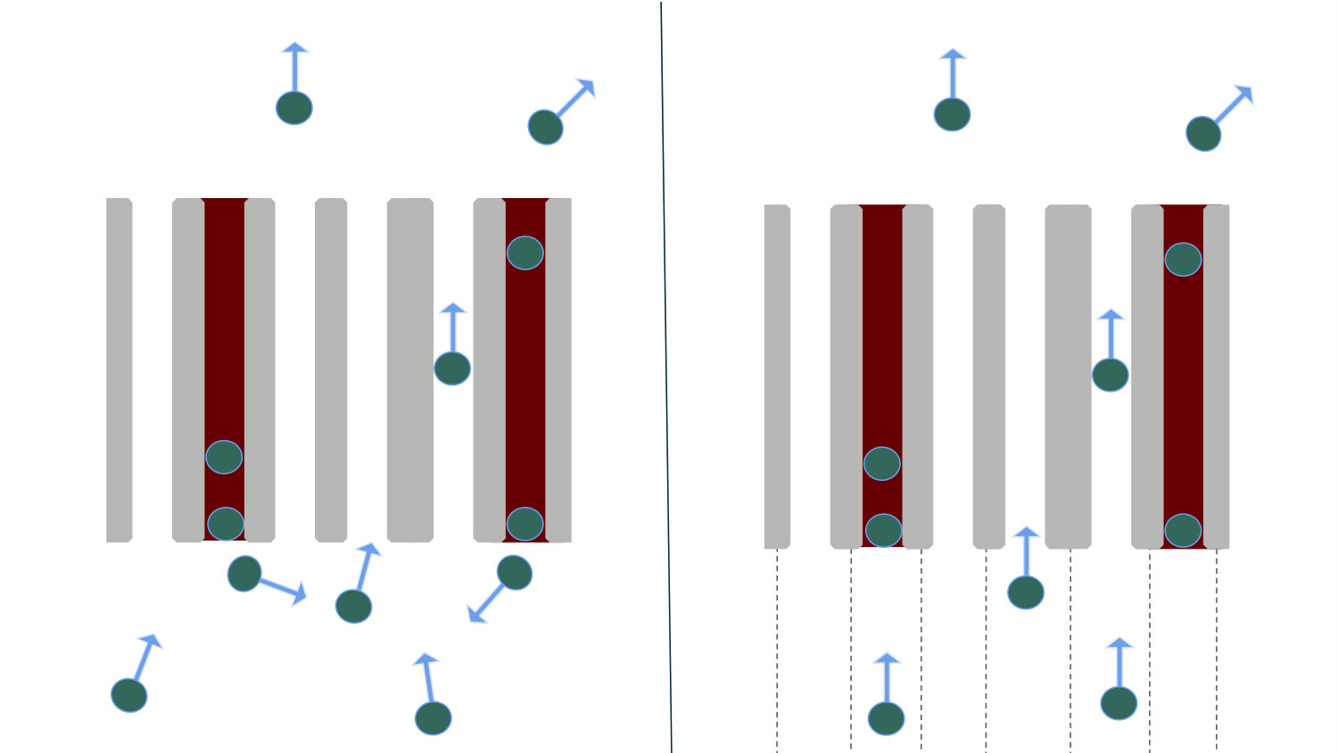 Figure 1
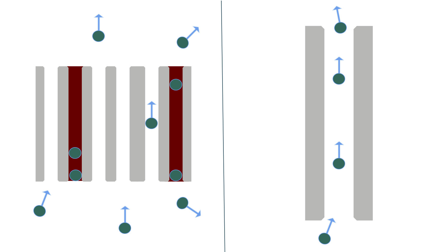 Figure 2
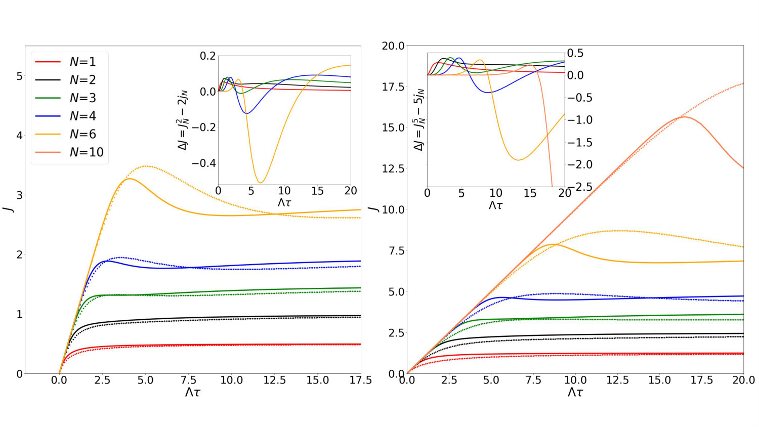 Figure 3
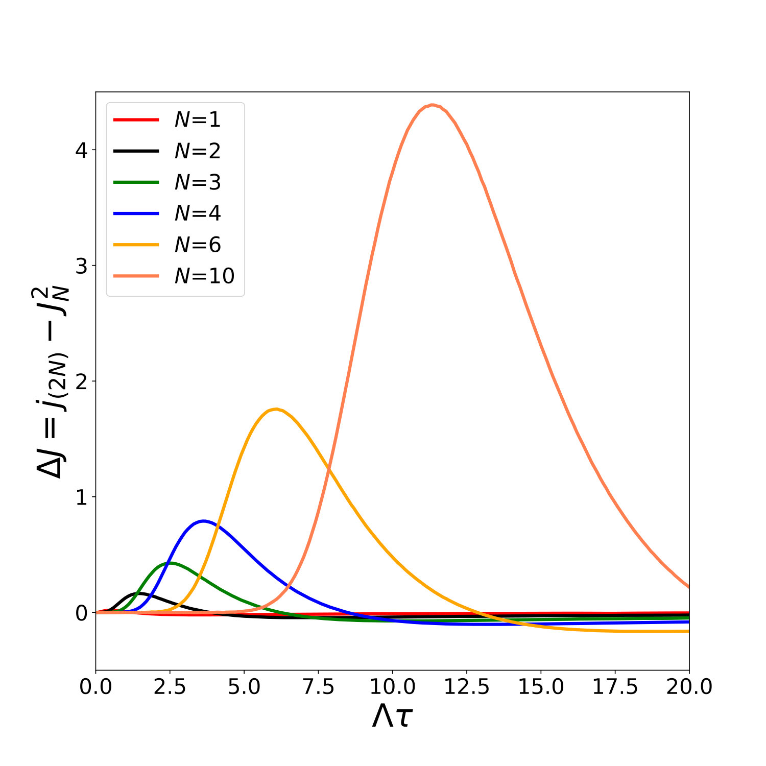 Figure 4
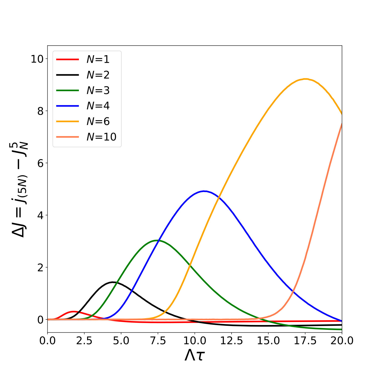 Figure 5
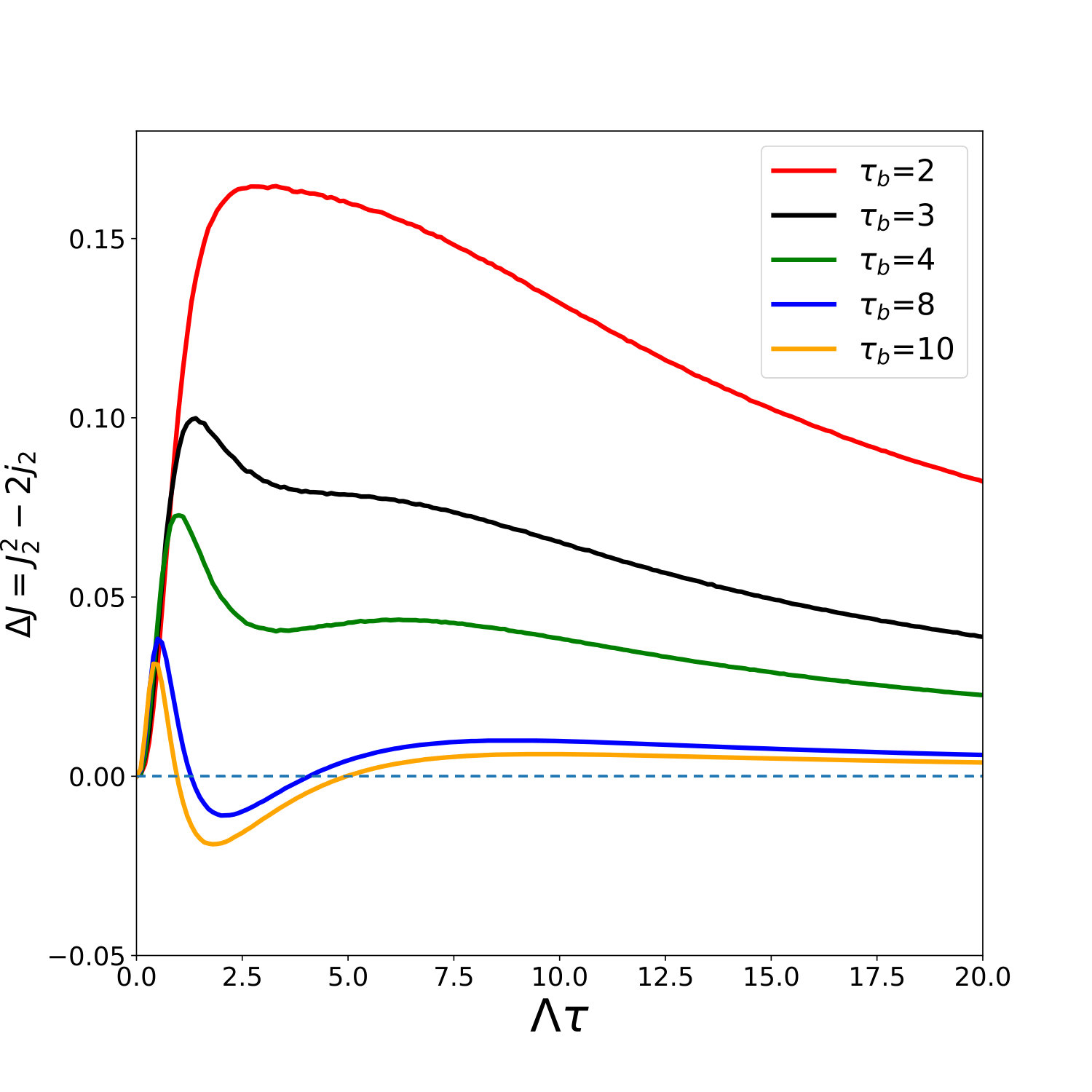 Figure 6
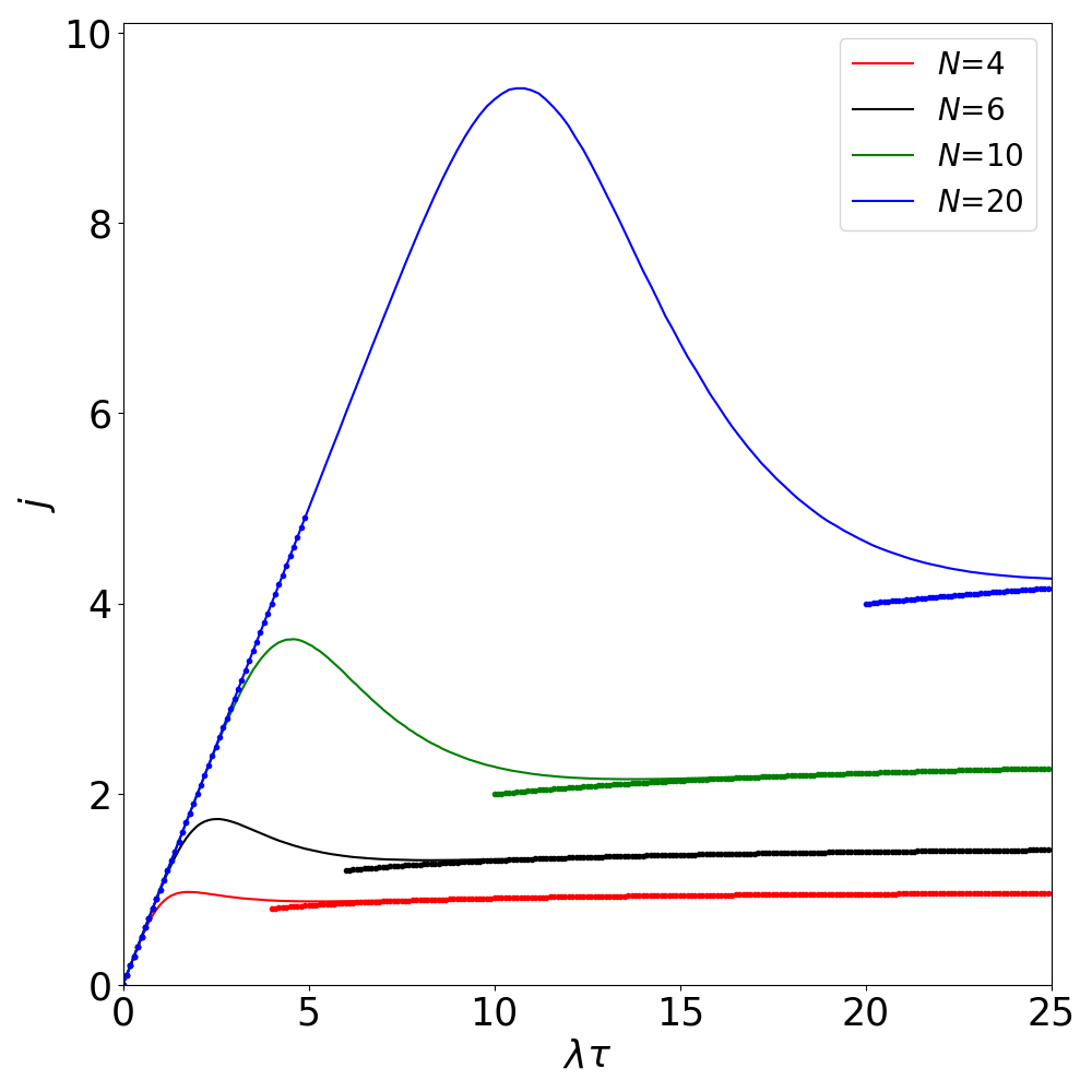 Figure 7
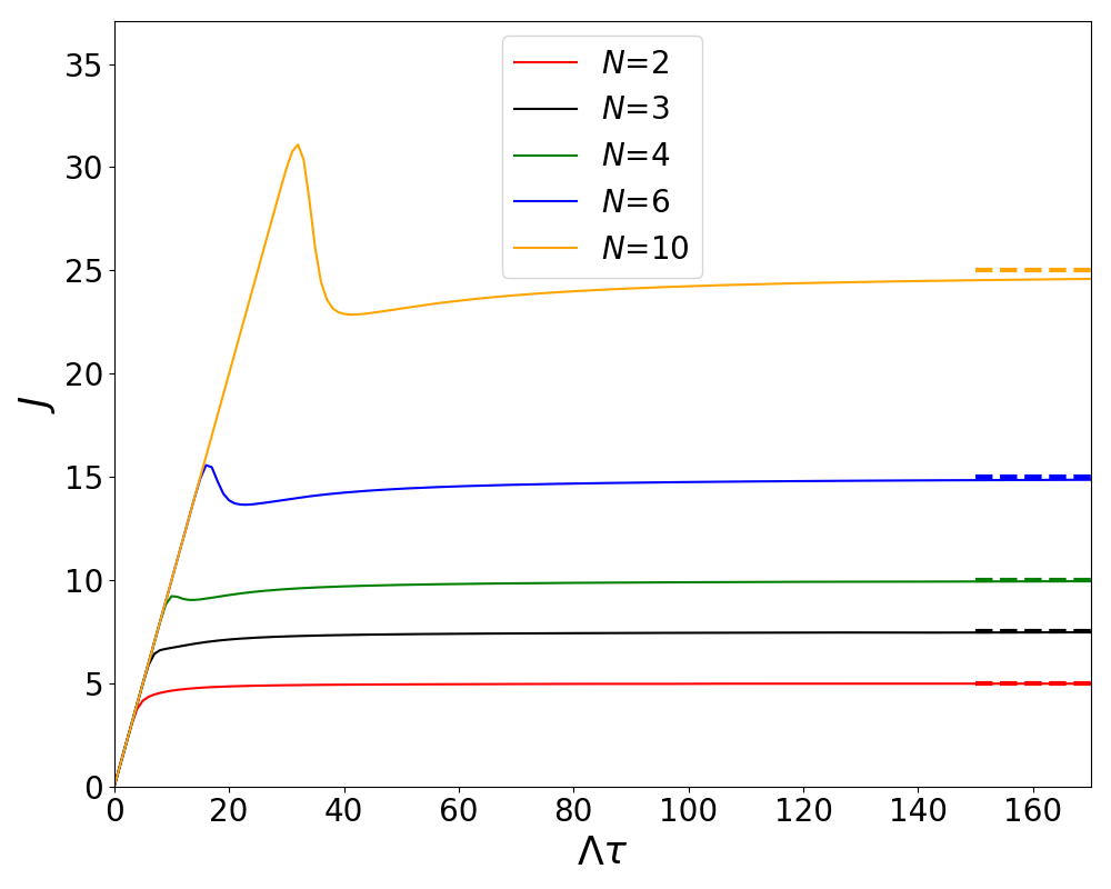 Figure 8
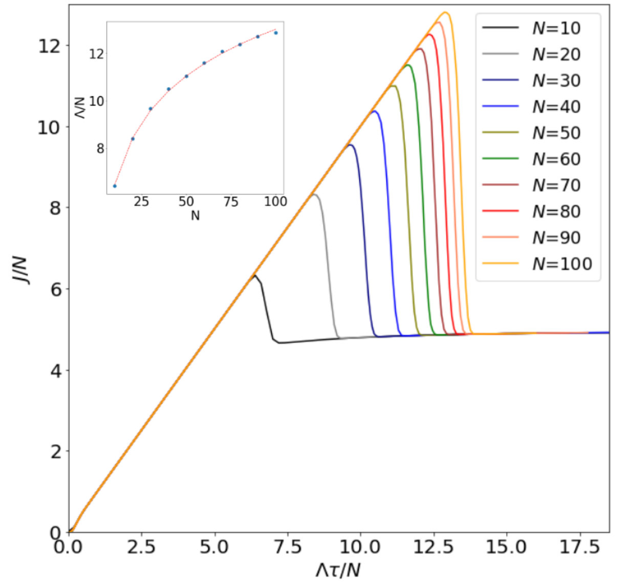 Figure 9
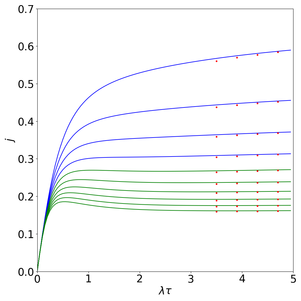 Figure 10
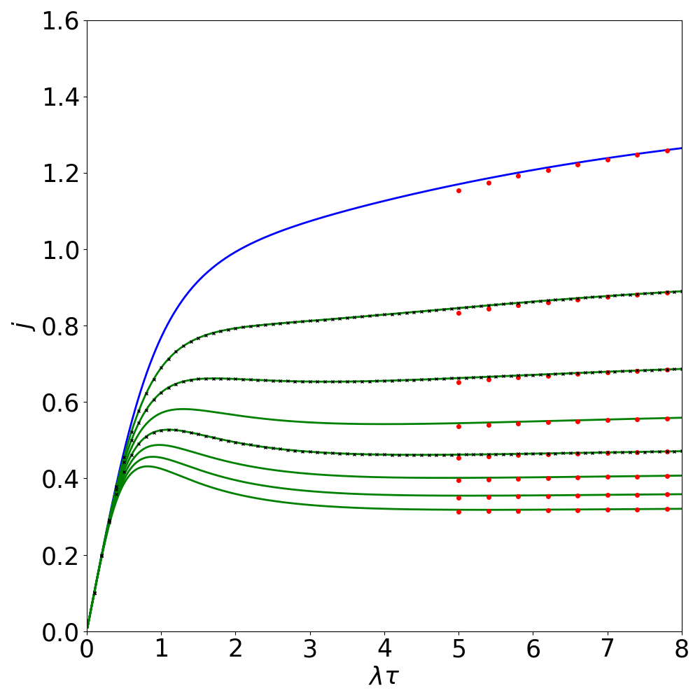 Figure 11
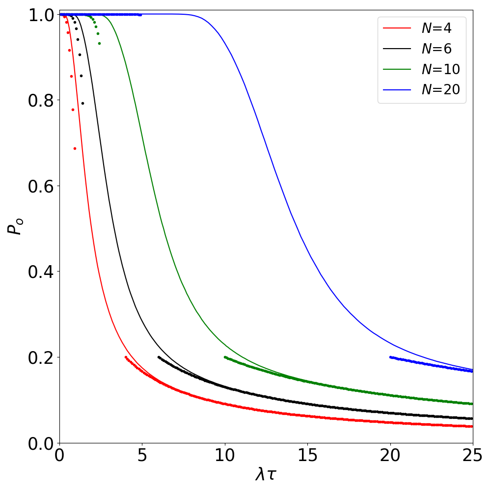 Figure 12
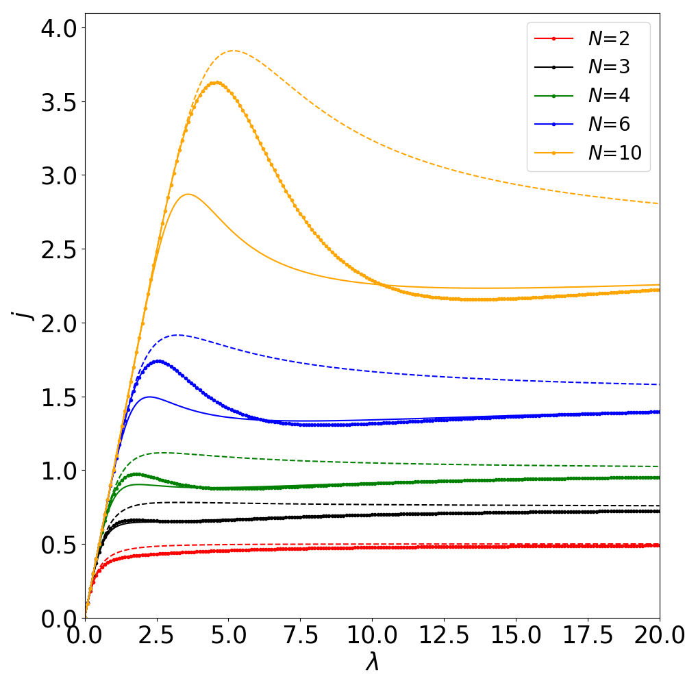 Figure 13
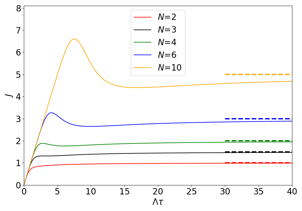 Figure 14
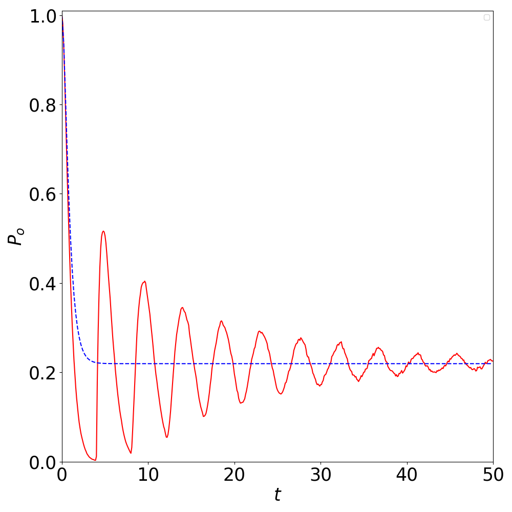 Figure 15
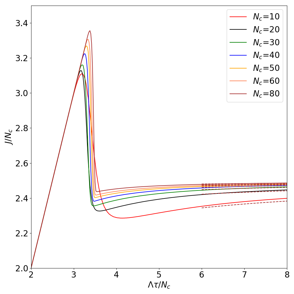 Figure 16
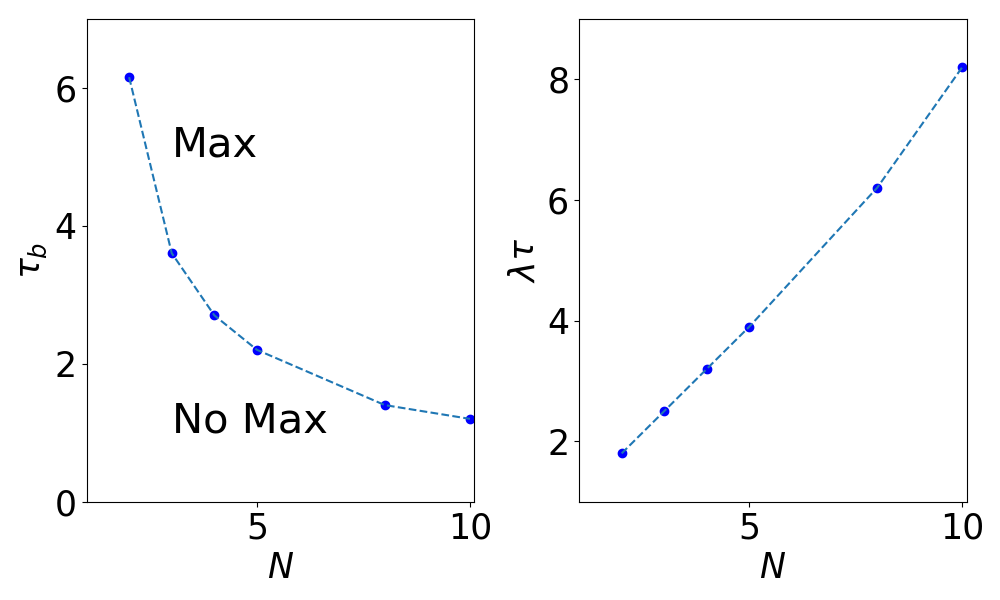 Figure 17
Peer Reviews
No public reviews on file for this paper yet. If you reviewed it on a platform where reviews are public (OpenReview, ICLR, NeurIPS, ICML), you can paste yours below so the community can read it here.
Videos
No videos yet. Explain this paper in a talk, walkthrough, or lecture? Add one.
Recurrence dynamics of particulate transport with reversible blockage:
from a single channel to a bundle of coupled channels
Chloé Barré, Gregory Page, Julian Talbot and Pascal Viot
Laboratoire de Physique Théorique de la Matière Condensée, SU, CNRS UMR 7600, 4, place Jussieu, 75005 Paris Cedex 05, France
Abstract
We model a particulate flow of constant velocity through confined geometries, ranging from a single channel to a bundle of identical coupled channels, under conditions of reversible blockage. Quantities of interest include the exiting particle flux (or throughput) and the probability that the bundle is open. For a constant entering flux, the bundle evolves through a transient regime to a steady state. We present analytic solutions for the stationary properties of a single channel with capacity and for a bundle of channels each of capacity . For larger values of and , the system’s steady state behavior is explored by numerical simulation. Depending on the deblocking time, the exiting flux either increases monotonically with intensity or displays a maximum at a finite intensity. For large we observe an abrupt change from a state with few blockages to one in which the bundle is permanently blocked and the exiting flux is due entirely to the release of blocked particles. We also compare the relative efficiency of coupled and uncoupled bundles. For the coupled system is always more efficient, but for the behavior is more complex.
I Introduction
Many physical and biological processes feature particle flow in confined geometries. Examples include vehicular and pedestrian traffic Helbing (2003); Appert-Rolland et al. (2010), filtration of particle suspensions, and the flow of macromolecules or ions through micro- or nanochannels Finkelstein and Andersen (1981); Kelkar and Chattopadhyay (2007); Daiguji et al. (2004). In biology, an important example is flux regulation mediated by pore-forming membrane proteins. The transport of ions and water through these channels is primarily a single-file process, i.e. cations and water molecules cannot pass each other within the channel Daiguji et al. (2004). Moreover, these flux regulatory channels can be clogged by toxins or medicines, with significant consequences. Recent studies of tracer diffusion of biased (or active) particles in a crowded, narrow channel revealed a non-trivial relationship between the exerted force and the mean velocity, as well asymmetric density profiles of the environment Bénichou et al. (2018a); Bertrand et al. (2018); Krapivsky et al. (2014); Bénichou et al. (2018b).
Some information systems, such as telecommunication Senderovich et al. (2015) and computing networks Tadayon and Aissa (2014); Ezaki et al. (2015), as well as trunked mobile radio systems and air traffic Janssen and Van Leeuwaarden (2008); Barcelo et al. (1996); Masrub (2014) are also amenable to the channel description.
A blockage may be caused by either ‘extrinsic’ or ‘intrinsic’ mechanisms. The former refers to the situation where the number of particles present somehow exceeds the channel carrying capacity, and will be the focus of this article. The latter mechanism arises from collective effects such as encountered in filtration processes. In this case, while isolated particles can pass through a mesh hole, clogging occurs when two or more particles arrive in near concurrence, causing one to impede the other. This effect, due to the delicate interplay between the spatio-temporal closeness of the particles and the confining geometry, could be seen as setting the capacity of a channel to greater than one, which establishes a connection between both types of blocking mechanisms. A model based on this phenomenology successfully accounted for experimental data Roussel et al. (2007); Redner and Datta (2000). Various approaches, including the Totally Asymmetric Simple Exclusion Process (TASEP)Mallick (2011, 2015) have been applied to model these phenomena. Gabrielli et al. introduced a class of stochastic models in which blockages occur when the carrying capacity of a channel is exceeded Gabrielli et al. (2013, 2015). For these stochastic models, the particle velocity within the channels is identical, and the mean particle density is low enough to prevent exclusion effects. The blockage is triggered when the number of particles within the channel at a given time exceeds the channel capacity. The original model considered one channel with capacity , i.e., two particles must be simultaneously present in the channel to block the system. Particles enter at random times according to a Poisson process of intensity and exit, if no blockage occurs, after a fixed transit time . Subsequently, several generalizations were studied, including a higher blocking threshold () Barré et al. (2015), an inhomogeneous entering flux Barré and Talbot (2015a), and multiple channels Barré and Talbot (2015b, 2016). When the blockage is reversible, the system is reactivated after a constant waiting time, . This mechanism gives rise to a transient regime leading to a steady state Barré et al. (2013). In this article we associate the last two generalizations.
Queuing theory Adan and Resing (2002); Medhi (1991) provides an alternative description of reversible blocking phenomena. This framework is typically used to describe customers arriving at a server, according to one given distribution, and receiving service according to another distribution. If all the elementary steps are Markov processes, the time evolution of the state probabilities can be described by systems of linear differential equations. In accordance with this approach, we recently introduced Markovian models of blockage Page et al. (2018); Barré et al. (2018) for which exact solutions can be obtained.
This paper is organized as follows: We first consider the single channel model in Sec. II, for which exact solutions are available for , and simulation results for greater values of . We also compare our results with the previously introduced Markovian models. In Sec. III a channel bundle model consisting of identical channels each of capacity and sharing an incoming flux is presented. Exact results are obtained for , as well as numerical simulation results for larger values of . These allow us to observe and explain some results in the limit of large or . In Sec. IV, we compare the efficiency of different configurations of channels in conveying a particulate flux of given intensity. Finally, in Sec. V we summarize our results.
II Single channel Model
Particles with identical constant velocities, are injected into a channel of length , according to a Poisson distribution of mean intensity . Given no blockage occurs, the particle transit time is . An instantaneous blockage occurs if particles are simultaneously present, and lasts for time . In the limit , there is no steady state and the exiting flux falls to zero Barré et al. (2015). Here, we focus instead on reversible blockages, during which, the particles are retained, and no more may enter the channel. After the deblocking time, the channel instantaneously releases all particles, resetting to the empty state, thereby allowing new ones to enter. The dynamics is therefore a recurring cycle of alternating open and closed states, that ultimately leads to a stationary state.
In an average steady state recurrence cycle, the channel is open for an average time and blocked for a fixed time . The stationary probability that the system is open is therefore
[TABLE]
where the denominator represents the total mean time of a recurrence. The stationary output flux is then given by the ratio of the mean number of particles released during one cycle to the cycle period,
[TABLE]
is the mean number of output particles between two successive blockages. By equating the number of entering particles in one period to those exiting we obtain the following ‘number balance’
[TABLE]
Finally from the above three equations we deduce that
[TABLE]
The latter relation does not depend on the existence of a cycle, as it is the result of number conservation. The output flux is equal to the entering one minus the part that is rejected when the channel is in the closed state.
By taking the limit , the mean blockage time and the mean number of exiting particles between blockages behave asymptotically as and , respectively. Therefore, for a given , the probability that the channel is open is close to unity and the flux . Blockages rarely occur at low . In this limit, the mean blockage time can be estimated by noting that a blockage occurs when a batch of particles enters in a finite duration , leading to Barré et al. (2015). Expanding to first order gives
[TABLE]
When , blockages are very frequent, and both the mean number of exiting particles between blockages, , and mean time between blockages, , approach zero. The resulting flux consists entirely of successive releases of the blocked particles, and . In this limit, corresponds to the time necessary for particles to enter an empty channel, . The open probability and the flux in this high intensity limit are therefore
[TABLE]
and
[TABLE]
II.1 Solvable models:
For small capacities, , the time evolution of the process can be expressed by analytically tractable differential or integro-differential equations Barré et al. (2013). For larger values of , the time evolution cannot be solved by any known means.
We first consider , which corresponds to a stochastic switch. The transit time is an irrelevant variable because no particle can exit the channel without having already blocked it. For , it is possible for particles to pass through the channel without causing a blockage. Let denote the probability that the channel is open at time . Its time evolution obeys
[TABLE]
The loss term corresponds to the entrance of a particle at time , while the channel is open, causing the channel to block. The gain term corresponds to the exit of a particle that became blocked at time , with the subsequent reopening of the channel at time .
The mean output flux at time is given by
[TABLE]
which corresponds to the release of a blocked particle that entered at . Applying the time Laplace transform, , to Eqs.(8) and (9) gives,
[TABLE]
and
[TABLE]
Expanding the denominator of Eq.(10) in terms of , allows one to easily invert the Laplace transform, term by term, giving,
[TABLE]
where is the Heaviside function. The stationary open probability, , and flux, , can be obtained from Eqs.(10) and (11) by using ,
[TABLE]
and
[TABLE]
These results can be easily inferred from Eqs. (1) and (2) by setting and . The exiting particle flux is controlled by the incoming flux and the time of blockage .
We now consider the model, i.e. blockage occurs when two particles are simultaneously in the channel, for which exact results have already been obtained Barré et al. (2013). Here we propose an alternative, simpler derivation using the state probabilities of the channel. Let , denote the probability that an open channel contains zero or one particle respectively, and be the probability that it contains two particles and is therefore blocked. The time evolution of the process is given by
[TABLE]
with the following initial conditions:
[TABLE]
In Eq.(15), the loss term corresponds to the entrance of a particle in the empty channel at time . The two gain terms and correspond to a particle exiting the channel at time and a channel release (with a blockage occurring at time ), respectively. In Eq.(16), the two loss terms describe either a particle exiting the occupied channel at time or a particle entering the occupied channel. The gain term corresponds to a particle entering a free channel. In Eq.(17), the loss term corresponds to a channel release and the gain term to a particle entering a channel with one particle already inside. Summing the three equations verifies that the total probability is conserved: .
Taking the Laplace transform of Eqs.(15-17) gives
[TABLE]
These simultaneous equations may be solved to give
[TABLE]
where
[TABLE]
The mean exiting flux is the sum of two contributions: the exit of a particle from an open channel and the release of of two particles from a closed channel. is therefore given by
[TABLE]
By using Eqs.(22),(23), the Laplace transform of the output flux is
[TABLE]
As expected, we recover the results of Ref.Barré et al. (2013) and the time-dependent mean flux can be obtained by a Laplace inversion of Eq.(27).
We here focus on the key quantities, namely the stationary probability that the system is open and the mean flux . is the sum of the two stationary probabilities and , each obtained by evaluating with :
[TABLE]
and
[TABLE]
Figure 1 displays versus for different integer values of from to . The dashed lines correspond to the asymptotic values of the exiting flux . One first observes that the stationary flux reaches the asymptotic values more rapidly as increases. Moreover, displays a maximum when is larger than . It is possible to obtain the exact value of for which the flux displays a maximum at a finite value of Page et al. (2018) by solving . A real solution for exists if . Note that for the flux is always a monotonically increasing function of .
For , the complete kinetic description of the model is cumbersome so we restrict our attention to the stationary quantities for which analytical expressions have been obtained Barré et al. (2015). In particular, the mean time to blockage starting from an empty channel is given by
[TABLE]
for and
[TABLE]
for , where and (note that these correct the expressions given in Barré et al. (2015)).
The two stationary quantities and are obtained by inserting this result in Eqs.(1) and(2). Fig. 2 displays as a function of for different values of . There are several differences compared with the model. First, a maximum exiting flux occurs if the blockage time , which is significantly smaller for (). Second, the asymptotic values are reached at a lower value of , and finally, the intensity at which is maximum is also shifted towards larger intensity.
II.2 Simulation results:
As a result of strong time correlations between the transiting particles, it is not possible to obtain analytic solutions for . We therefore used numerical simulations to investigate these cases. In order to benchmark our code, we compared the simulation results for the stationary flux for with the exact expressions for three different values of . In Fig. 2 we observe perfect agreement between the analytical expressions and the simulation results.
Figure 3 displays the stationary exiting flux as a function of the intensity for different values of and . At low intensity, the flux increases linearly, and at high intensity the asymptotic behavior of the simulation results is well-desribed by Eq. (7). The behavior in the intermediate region is due to complex dynamics that alternates between blockages and sequences of uninterrupted transport. For , the stationary flux may display a maximum at finite , whose amplitude increases with . The stationary flux also exhibits a minimum which is always smaller than the asymptotic value, .
We performed a systematic study of the behavior of the exiting flux as a function of and . The flux always displays a maximum when exceeds a threshold value. Figure 4 shows that the critical value of decreases rapidly with , showing that the feature observed in Fig. 1 is very general and occurs for smaller values of when increases. For below the critical value, the stationary flux is a monotonically increasing function of . The right panel of Fig. 4 shows the values of corresponding to the critical values of .
The behavior of the open probability , shown in Fig. 5, is consistent with Eq. (4). In particular one observes the appearance of a plateau whose length increases with (roughly as ). This corresponds to the situation where blockage events are rare and the output flux is close to .
II.3 Markovian versus non-Markovian models
The physical assumption of constant transit and deblocking times and , respectively, is responsible for strong memory effects which prevent analytical solutions for general from being obtained. We therefore recently introduced Markovian models Page et al. (2018); Barré et al. (2018), where the average transit and deblocking times are stochastic variables given by exponential distributions of intensity and , respectively. The kinetic description of the Markovian model is given by a set of differential equations for the time evolution of the state probabilities with giving the number of particles in the channel. Unlike the non-Markovian model, analytic solutions for the steady state properties can be obtained for arbitrary (some generalizations of the Markovian models for which time-dependent solutions can be obtained and could be investigated in the future Leonenko (2009); Escobar et al. (2002)).
The channel is open for an mean time and blocked for a mean time . The stationary flux is obtained using the previously employed recurrence arguments, giving
[TABLE]
The average time for which the Markovian system is open in a recurrence cycle is Page et al. (2018)
[TABLE]
To compare the two models, and must be related to , and . Eq. (32) with Eq. (2) shows that must equal . To obtain an expression for , we consider the system’s behavior at low and high intensity. When , the non-Markovian transit time is equal to . The mean transit time is in the the Markovian model. A first approach is to therefore set . When , we expect to decrease to zero. Figure 6 shows that the stationary flux of the Markovian model is always larger than that of the non-Markovian model. Even though the two models behave similarly at small and large input intensity, they increasingly deviate for intermediate intensities with increasing .
To obtain an exact mapping (in the steady state) we equate the mean blocking time of the two models. For we equate given by Eq. (33) with the result for the non-Markovian model Gabrielli et al. (2013), . The expressions are identical when
[TABLE]
With this mapping, we recover the aforementioned expected limiting behaviour for both extremes of entering flux intensity. We emphasize that the transient regimes of the two models are different (See the Appendix A for a similar model where time-dependent analytic solutions are obtained).
The same procedure can be carried out for using Eqs. (30) and (31), but the resulting expression for is considerably more complex. For general we therefore propose the following ansatz, taking a similar form as the mapping for :
[TABLE]
which behaves as at low intensity and approaches zero exponentially at large intensity. Substituting Eq.(35) into Eq.(32), produces a lower bound of the stationary flux (full curves). Furthermore, the maximum of the flux is underestimated and shifted to a smaller intensity than in the non-Markovian model. For and , the curves are very close to the results of the non-Markovian model. For , the ansatz leads to a significant underestimation of the exiting flux for small .
III Bundle model
We now consider a bundle of identical channels. Each channel has the same properties as the single channel model above, i.e. blockage occurs when particles are present in a channel at the same time. In the following we assume that the total intensity, , is constant and is equally distributed over the open channels. Thus, after blockages the intensity on each of these open channels is
[TABLE]
Since a blocked channel releases all particles after finite time , the system’s mean output flux evolves towards a non-zero stationary value. The bundle has two states: open in which at least one of the constituent channels is open and closed if all the constituent channels are blocked. If a particle arrives while the bundle is in the latter state, it is rejected.
Equations (1,2,3) cannot be applied to the channel bundle in the steady state, as it does not cycle between closed and empty states for finite intensity . In the limit of very large intensities, however, we have
[TABLE]
and
[TABLE]
where is the mean number of exiting particles that are not the due to blockage releases, and
[TABLE]
In this limit the intensity is so high that all channels block instantaneously and simultaneously and the blocked particles are released after a time . The exiting flux is entirely the result of these releases.
The analogue of Eq. (4),
[TABLE]
is valid for arbitrary intensity since, as for the single channel case, it is result of the conservation of particle number.
III.1 Exact solution:
When a particle may traverse the channel in a time without causing a blockage. In comparison, the model is singular as no unimpeded transit is possible: each entering particle causes a blockage that lasts for a fixed time, . The variable is thus absent in this model.
Despite the relative simplicity of the model, its dynamics cannot be written as a system of differential equations for the state probabilities , where denotes the number of blocked channels at time (in Appendix A the full time dependent solution for is presented). However, in the stationary state, by applying detailed balance (known as the “rate up - rate down” principle in queuing theory), one has
[TABLE]
Solving the difference equation and applying conservation of the total probability leads to
[TABLE]
The stationary exiting flux is given by Eq. (40) with
[TABLE]
The result can be written in the form
[TABLE]
where is the incomplete gamma function. The asymptotic behavior at small intensity is
[TABLE]
whereas at large intensity the flux behaves as,
[TABLE]
whose leading term is in accordance with Eq. (39). For all values of , is always a monotonically increasing function of .
We note that the expression for is Erlang’s first formula Takacs (1969); Medhi (1991) for a stochastic queuing process with servers with exponential entry and service time distributions under the condition that when all servers are busy an arrival is rejected. Both models are ‘birth-and-death’ processes that have the same stationary solution. Their transient regimes, however, are significantly different. See Appendix A.
III.2 Simulation results:
For the multichannel models, no exact solution can be obtained for . Therefore we have performed numerical simulations to obtain the stationary exiting flux, and the stationary probability that at least one channel is open, for bundles composed of different numbers of channels with increasing capacity and for . All quantities were investigated as a function of the mean incoming flux . As discussed in the previous section, the stationary flux rapidly displays a maximum at a finite value of when .
Figure 7 shows as a function of for and for . When , the rate of incoming particles is very small and the finite capacity of the channel is rarely reached, meaning that blockage events are scarce. The stationary exiting flux is therefore equal to the input flux, . This behavior is observed for a larger range of for larger values of and .
Figure 8 shows the rescaled flux versus the rescaled intensity for different values of . In the low intensity regime is equal to and displays a finite discontinuity at . At high intensities the curve evolves towards an asymptote and is quite well described by
[TABLE]
We observe an abrupt change of kinetic behavior: Below the critical value , almost all particles cross the bundle without triggering a significant number of blockages, whereas for larger , all channels are closed and the stationary flux is essentially given by the release of blocked particles.
Fig. 9 shows the rescaled flux versus the rescaled intensity for different values of for a given . At a low input intensity, the exiting flux is equal to until it reaches a maximum close to a critical value that closely follows a logarithmic law, as shown in the inset of Fig. 9. For higher values of input intensity, the rescaled exiting flux, for all values of , rapidly collapses to a single curve, whose best fit is again given by Eq. (47).
IV Flux optimization
Here we compare the stationary flux of a bundle of coupled channels with that of a bundle of uncoupled channels and one high capacity (HC) channel. The transport efficiency is measured by the difference in output flux, . The systems are chosen so that in the limits of low and high input flux intensity, . In the low intensity limit, since blocking events are rare, the exiting flux is equal the input flux , irrespective of the configuration. In the high intensity limit, Eqs.(6) and (39) demonstrate that the exiting fluxes of the single high capacity, bundled uncoupled or coupled channels are also be equal. Since the stationary flux of a bundle of coupled channels displays non-trivial behavior with increasing and , we therefore expect non-trivial behavior of .
IV.1 Coupled versus uncoupled channels
We first compare a channel bundle composed of channels, each of capacity . The entering flux, , is equally distributed over the coupled open channels. In contrast, the independent channels, each of capacity , each receive an incoming flux of intensity . Fig. 10 illustrates the configurations compared. The difference in the output flux of the two configurations is defined as:
[TABLE]
Simulation results comparing the output flux of each configuration for , , are shown in Fig. 11. The differences are shown in the inset of the figure. At low intensity, for all configurations, the output flux is approximately equal for each setup, and linearly increases with until a critical value, which itself is a monotonically increasing function of .
The behavior for can be understood quantitatively using the results of Sec. III.1 and Eq. (14). At low intensity, the flux difference is
[TABLE]
and at high density we find
[TABLE]
and one can confirm that for . We conclude that the coupled channels are always more efficient than the uncoupled ones. The difference is maximized for a finite value of .
For all , we note the appearance of two maxima in the flux difference with an intervening minimum. The increased complexity is due to the presence of two characteristic times, the transit time and the blockage time (while the system has only the latter).
Fig. 12 shows the flux difference between the bundle configurations at , , as a function of intensity of entering flux, , for different values of . For the behavior is more complex after the first maximum, with the appearance of a minimum followed by a second maximum before tending towards zero.
IV.2 Single HC channel verses coupled LC channels
The transport efficiency of a single ’high capacity’ (HC) channel, with a bundle of several coupled channels, of a proportionately reduced capacity, is now compared. The two configurations are illustrated in Fig. 13. Figure 14 shows the difference in the output stationary state flux between a single HC channel and a bundle of coupled LC channels, with different capacities. The flux difference in this case is
[TABLE]
For all , the flux difference displays a minimum, followed by a maximum, before tending towards zero for increasing intensity. The amplitudes of the maxima are always greater than those of the minima.
V Discussion
We have presented a model of blockage in channel bundles that may be relevant for various physical processes. The bundle consists of constituent channels, each with a capacity of . A particle transits through an open channel in time , but if particles are simultaneously present in a channel, it is blocked for a time , before being emptied. While blocked, the entering flux is redistributed over the remaining open channels. A bundle of channels is open if at least one of its constituent channels is not blocked. If the entering stream is of constant intensity the bundle evolves to a stationary state with a steady exiting flux, or throughput, that depends on the intensity, and . In the steady state the exiting flux is simply related to the probability that the bundle is open. For a single channel with capacity the exiting flux displays a maximum value at finite intensity if is sufficiently large. If not, the exiting flux increases monotonically with the intensity. A Markovian model with stochastic transit and blockage times, inspired by queuing theory, can be made to display the same steady state behavior with an appropriate mapping between the two models’ parameters. The transient behavior is, however, quite different. This suggests that, in the steady state, the details of the transport mechanisms and the triggered releases are not important. For large , the models display an abrupt change from a state with few blockages to one in which the bundle is permanently blocked and the output flux is entirely due to the release of blocked particles. This behavior raises new questions about whether more general relationships describing the abrupt transitions in dynamics may be obtained for general and . The transport efficiency of a bundle in which the entering flux is equally distributed over the open channels was also compared with a bundle composed of independent channels. For , the coupled channels always have a higher throughput, but for larger values of the behavior is more complex.
Acknowledgements.
We thank Jacques Resing, Karim Guerouate et Valentin Wiener for useful discussions.
Appendix A Full Solution of the Channel Bundle with ,
This model can be solved exactly by using an approach similar to that used to solve the single channel model with Barré et al. (2015). This requires introducing the partial probabilities that at time , particles have entered such that at least one channel is open. The open probability of the bundle is then given by
[TABLE]
Since blockage is not possible for the first two probabilities are trivial:
[TABLE]
For , the probability can be written as:
[TABLE]
The -fold integral corresponds to all events of incoming articles at the entry of the channel with the associated constraint ( function) which occurs between [math] and . The first product of Heaviside functions expresses the fact that a new particle can enter if both channels are not blocked, which imposes the condition that the time since the entry of the second last particle is larger than ; The last product corresponds to both complementary situations: either the last entered particle leads to a complete blockage of two channels (The exponential factor expresses that no particle can enter in a duration ) or only one channel is blocked by the last entered particle. The last Heaviside function imposes the requirement that at least one channel be open at time .
Taking the Laplace transform of , the integral over is trivial and the integral over must be split into two parts, which finally gives
[TABLE]
with . The function is defined as
[TABLE]
By using Eq.(57), one infers the recurrence relation between and
[TABLE]
with the initial condition
We define the generating function
[TABLE]
Multiplying Eq. (58) by and summing over , gives the generating function obeys to a similar equation
[TABLE]
For , the right-hand side of Eq.(A) is independent of , which gives that is then independent of . For , by taking the two first derivatives of Eq.A with respect to , one can rewrite the integral equation, Eq.(A) as an ordinary differential equation
[TABLE]
whose solution is given by
[TABLE]
where and are the solutions of the characteristic equation
[TABLE]
The functions and are determined by using the boundary conditions. At , by using Eq. (A), is expressed as
[TABLE]
which gives
[TABLE]
Now, by using the first derivative of Eq. (A) at , one obtains the second boundary equation
[TABLE]
and by using Eq.(62), one obtains
[TABLE]
In the Laplace space, the open probability is given by
[TABLE]
By using Eq.(A) and Eq.(62), this can be expressed as
[TABLE]
The functions and can be determined by using the boundary conditions, but the lengthy expressions are not displayed here. The output flux is entirely due to the release of blocked particles and is therefore given by
[TABLE]
The stationary open probability is . By using Eq.(69), the stationary open probability is then given by
[TABLE]
After a tedious but straightforward calculation, one finally obtains
[TABLE]
which corresponds to the Erlang formula, Eq. (43).
Let us now compare with the stochastic model with and with parameters and . The state of the system is defined by the probabilities , , of having zero, one and two particles in the bundle at time , respectively. They evolve according to the coupled differential equations
[TABLE]
Taking the Laplace transform, and solving the linear system of algebraic equations, one obtains the Laplace transform of the open probability,
[TABLE]
Finally, calculating the inverse Laplace transform and substituting , one obtains
[TABLE]
with .
Figure 15 shows the time evolution of the open probability, , of the non-Markovian model and of the stochastic model for and . While both models converge to the same stationary state (with the same open probability and output fluxes), the relaxation is significantly different, except at short time (typically for ). In particular, for the non-stochastic model, the deterministic blockage release mechanism leads to slow, oscillatory relaxation towards the stationary state, whereas the relaxation is roughly exponential and faster for the stochastic model.
The reference list from the paper itself. Each links out to its DOI / PubMed record.
- 1Helbing (2003) Dirk Helbing, “Modelling supply networks and business cycles as unstable transport phenomena,” New Journal of Physics 5 , 90 (2003) .
- 2Appert-Rolland et al. (2010) C Appert-Rolland, H J Hilhorst, and G Schehr, “Spontaneous symmetry breaking in a two-lane model for bidirectional overtaking traffic,” J. Stat. Mech. 2010 , P 08024 (2010) .
- 3Finkelstein and Andersen (1981) Alan Finkelstein and Olaf Sparre Andersen, “The gramicidin a channel: A review of its permeability characteristics with special reference to the single-file aspect of transport,” The Journal of Membrane Biology 59 , 155–171 (1981) . · doi ↗
- 4Kelkar and Chattopadhyay (2007) Devaki A. Kelkar and Amitabha Chattopadhyay, “The gramicidin ion channel: A model membrane protein,” Biochimica et Biophysica Acta (BBA) - Biomembranes 1768 , 2011 – 2025 (2007) . · doi ↗
- 5Daiguji et al. (2004) Hirofumi Daiguji, Peidong Yang, and Arun Majumdar, “Ion transport in nanofluidic channels,” Nano Lett. 4 , 137–142 (2004) . · doi ↗
- 6Bénichou et al. (2018 a) O Bénichou, P Illien, G Oshanin, A Sarracino, and R Voituriez, “Tracer diffusion in crowded narrow channels,” Journal of Physics: Condensed Matter 30 , 443001 (2018 a) .
- 7Bertrand et al. (2018) Thibault Bertrand, Pierre Illien, Olivier Bénichou, and Raphaël Voituriez, “Dynamics of run-and-tumble particles in dense single-file systems,” New Journal of Physics 20 , 113045 (2018) .
- 8Krapivsky et al. (2014) P. L. Krapivsky, Kirone Mallick, and Tridib Sadhu, “Large deviations in single-file diffusion,” Phys. Rev. Lett. 113 , 078101 (2014) . · doi ↗