
TL;DR
This paper constructs an infinite stable looptree, proves its emergence as a limit of discrete and compact looptrees, and analyzes its geometric and stochastic properties, including volume growth and Brownian motion behavior.
Contribution
It introduces the infinite stable looptree and establishes its role as a limit object in various discrete and compact settings, along with spectral and stochastic analysis.
Findings
Infinite stable looptree constructed and characterized.
Proven as a local and scaling limit of discrete and compact looptrees.
Analyzed spectral dimension and Brownian motion on the infinite looptree.
Abstract
We give a construction of an infinite stable looptree, which we denote by , and prove that it arises both as a local limit of the compact stable looptrees of Curien and Kortchemski (2015), and as a scaling limit of the infinite discrete looptrees of Richier (2017) and Bj\"ornberg and Stef\'ansson (2015). As a consequence, we are able to prove various convergence results for volumes of small balls in compact stable looptrees, explored more deeply in a companion paper. We also establish the spectral dimension of , and show that it agrees with that of its discrete counterpart. Moreover, we show that Brownian motion on arises as a scaling limit of random walks on discrete looptrees, and as a local limit of Brownian motion on compact stable looptrees, which has similar consequences for the limit of…
Click any figure to enlarge with its caption.
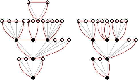 Figure 1
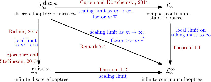 Figure 2
 Figure 3
 Figure 4
 Figure 5
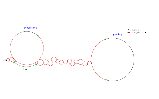 Figure 6
 Figure 7
 Figure 8
 Figure 9
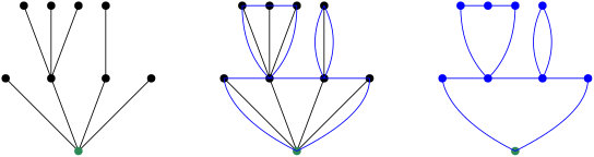 Figure 10
 Figure 11
 Figure 12
 Figure 13
 Figure 14
 Figure 15
 Figure 16
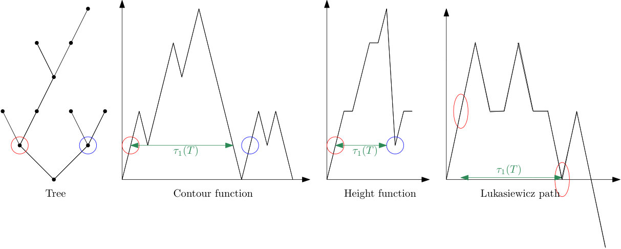 Figure 17
 Figure 18
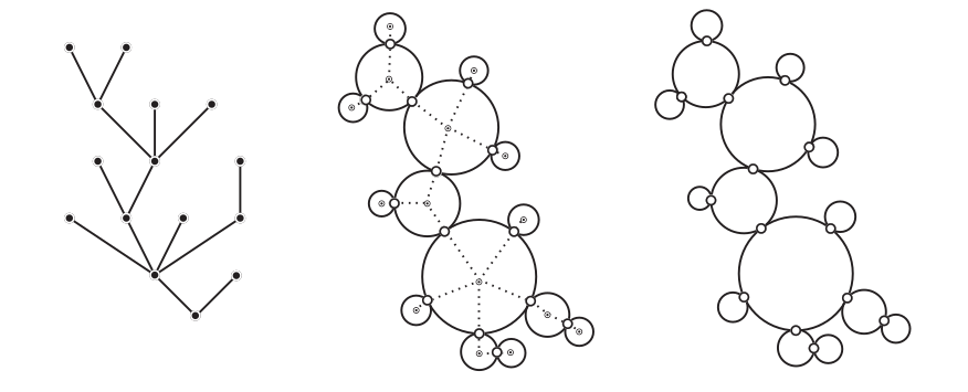 Figure 19
 Figure 20
 Figure 21
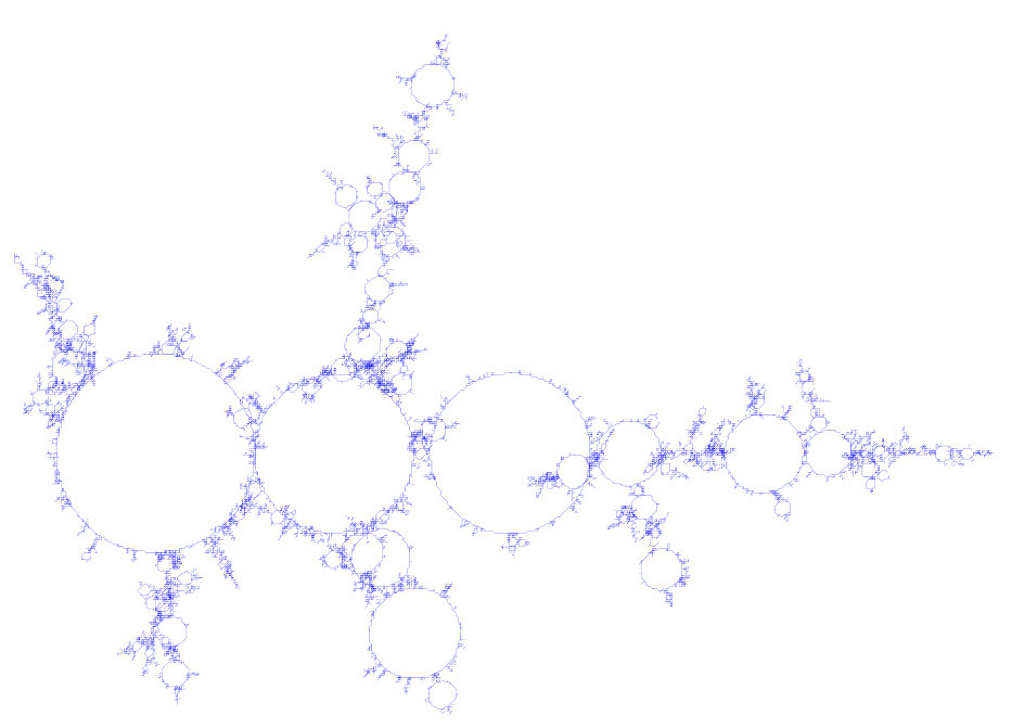 Figure 22
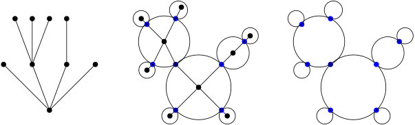 Figure 23
 Figure 24
 Figure 25
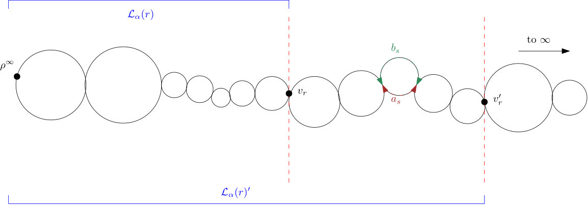 Figure 26
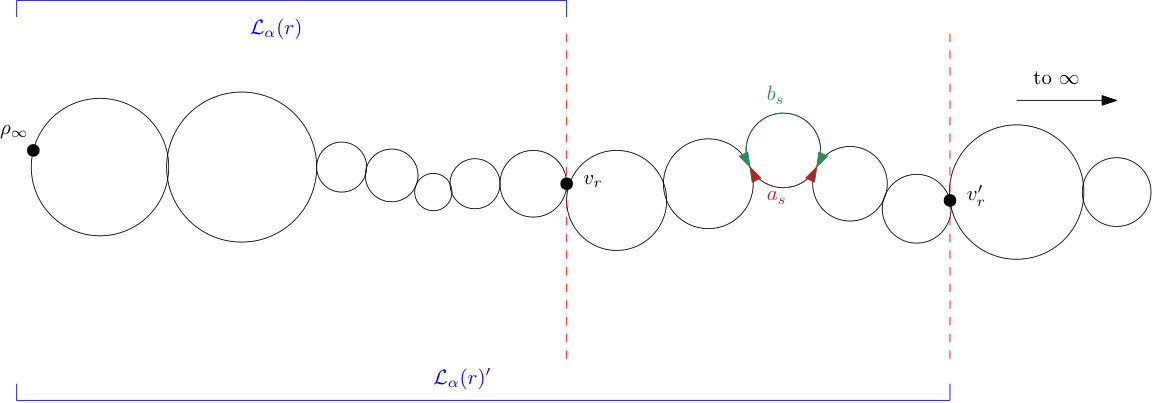 Figure 27
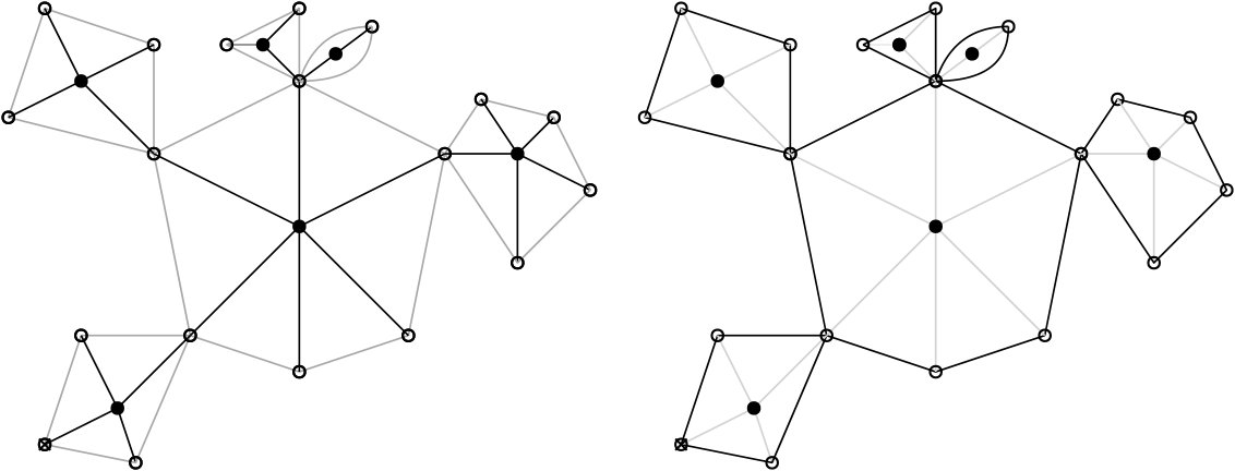 Figure 28
Peer Reviews
No public reviews on file for this paper yet. If you reviewed it on a platform where reviews are public (OpenReview, ICLR, NeurIPS, ICML), you can paste yours below so the community can read it here.
Videos
No videos yet. Explain this paper in a talk, walkthrough, or lecture? Add one.
Infinite stable looptrees
Eleanor Archer Mathematics Institute, University of Warwick, Coventry CV4 7AL, United Kingdom. Email: [email protected]. Supported by EPSRC Grant Number EP/N509796/1.
Abstract
We give a construction of an infinite stable looptree, which we denote by , and prove that it arises both as a local limit of the compact stable looptrees of Curien and Kortchemski (2015), and as a scaling limit of the infinite discrete looptrees of Richier (2017) and Björnberg and Stefánsson (2015). As a consequence, we are able to prove various convergence results for volumes of small balls in compact stable looptrees, explored more deeply in a companion paper. We also establish the spectral dimension of , and show that it agrees with that of its discrete counterpart. Moreover, we show that Brownian motion on arises as a scaling limit of random walks on discrete looptrees, and as a local limit of Brownian motion on compact stable looptrees, which has similar consequences for the limit of the heat kernel.
AMS 2010 Mathematics Subject Classification: 60F17 (primary), 60K37, 54E70, 28A80
Keywords and phrases: random stable looptrees, limit theorem, spectral dimension, stable Lévy process.
1 Introduction
Stable looptrees are a class of random fractal objects indexed by a parameter and can informally be thought of as the dual graphs of stable trees. Motivated by [LGM11], they were originally introduced by Curien and Kortchemski in [CK14], and along with their discrete counterparts have been shown to be of increasing significance in the study of statistical mechanics models on random planar maps. For example, the same authors showed in [CK15] that a stable looptree arises as the scaling limit of the boundary of a critical percolation cluster on the UIPT, and Richier showed in [Ric18a] that the incipient infinite cluster of the UIHPT has the form of an infinite discrete looptree. Further results along these lines can be found in [CK15], [CDKM15], [SS19], [BR18], [CR18] and [KR], though this is a very non-exhaustive list. More generally, they also arise as the scaling limits of boundaries of stable maps [Ric18b], and are emerging as an important tool in the programme to reconcile the theories of random planar maps and Liouville quantum gravity, demonstrated for example in [MS15], [GP] and [BHS18].
Given a discrete tree , the corresponding discrete looptree as defined in [CK14] is constructed by replacing each vertex with a cycle of length equal to the degree of in , and then gluing these cycles along the tree structure of . This is illustrated in Figure 1. This operation can also be applied in the case where is an infinite tree. If is rooted, we will take the convention that the root of is the vertex of corresponding to the edge of joining the root of to its first child.
In this article we will mainly be interested in the case where our tree has a critical offspring distribution in the domain of attraction of an -stable law, by which we mean that there exists an increasing sequence such that, if are i.i.d. copies of , then
[TABLE]
as , where is an -stable random variable (and can be normalised so that for all ). It is shown in [BGT89, Section 8.3.2] that necessarily for some slowly-varying function , where we recall that slowly varying means that for all sufficiently large , and for all .
Equivalently, . In the case where as , we can take .
Throughout the article we will make the assumption that . In [CK14, Theorem 4.1], it is shown that if is a Galton Watson tree conditioned to have vertices with offspring distribution in the domain of attraction of an -stable law, then we can define the -stable looptree (which we denote by ) to be the random compact metric space such that
[TABLE]
in the Gromov-Hausdorff topology as . A simulation is shown in Figure 2. In the case , the looptrees instead rescale to the Brownian Continuum Random Tree [KR19, Theorem 2].
The main purpose of this paper is to give a construction of infinite stable looptrees. The construction is similar in spirit to Duquesne’s construction of stable sin-trees in [Duq09], which is the continuum analogue of Kesten’s discrete construction of an infinite critical tree. Additionally, infinite discrete looptrees have been defined by Björnberg and Stefánsson in [BS15] by applying a related loop operation to Kesten’s infinite critical tree , and similarly by Richier in [Ric18a] by applying a similar operation to a two-type version of Kesten’s tree.
As is done for stable sin-trees in [Duq09], we define the infinite stable looptree from two independent stable Lévy processes, each of which is used to code the looptree on one side of its singly infinite loopspine. This is the construction suggested in [Ric18a, Section 6] and is the natural extension of the coding mechanism used to define stable looptrees from stable Lévy excursions.
The construction is given in Section 4. The remainder of the article is devoted to proving various limit theorems to justify the definition, and then using these to make deductions about Brownian motion on compact stable looptrees, which is explored more deeply in the companion paper [Arc19]. In particular, we prove a local limit theorem showing that can be characterised as the local limit of compact stable looptrees, and also as the scaling limit of infinite discrete looptrees. When combined with earlier results of Curien and Kortchemski, Björnberg and Stefánsson, and Richier, this shows that the diagram of Figure 3 commutes as indicated.
We start by giving the local limit result. In what follows, we let be a compact stable looptree conditioned to have total volume , and let be as above. We recall from [CK14] that is endowed with a measure which can be thought of as the natural analogue of uniform measure on . We will define a similar measure on in Section 4, and denote it by . We also recall from [CK14] (respectively [Arc19]) that there is a natural way to define shortest-distance metric (respectively a resistance metric) on , and we will define analogous metrics for in Section 4.
Theorem 1.1**.**
Let be a compact stable looptree conditioned to have mass , and let be as above. Then,
[TABLE]
as , with respect to the Gromov-Hausdorff-vague topology. Here and can denote either the geodesic metrics, or the effective resistance metrics on the respective spaces.
Similarly, we prove the following scaling result.
Theorem 1.2**.**
Let denote Kesten’s tree with critical offspring distribution in the domain of attraction of an -stable law. Also let denote the measure that gives mass to every vertex of Loop(). Then
[TABLE]
with respect to the Gromov-Hausdorff vague topology as . Here and can denote either the geodesic metrics, or the effective resistance metrics on the respective spaces.
We will see in Section 5.2 that similar results hold for the infinite discrete looptrees defined in [BS15] and [Ric18a].
Given these two theorems, we are also in the right setting to apply results of [Cro18] regarding limits for stochastic processes on these spaces. In particular, we obtain the following results. Note that we formally define Brownian motion on stable looptrees in the article [Arc19] by defining it to be the stochastic process naturally associated with the effective resistance metric on them. In Section 4, we similarly define an effective resistance metric on and in Section 7 we define Brownian motion on to be the associated stochastic process. We denote it by . For convenience, we restrict to the case where takes integer values below, but the result holds along any countable subsequence diverging to infinity.
Theorem 1.3**.**
Let be Brownian motion on , and let be Brownian motion on . Then there exists a probability space on which we can almost surely define a metric space in which the spaces and can all be embedded and such that
[TABLE]
with respect to the Gromov-Hausdorff-vague topology as , and the required Hausdorff convergence specifically holds in the metric space . Letting and be as above, we have that
[TABLE]
as , considered on the space endowed with the topology of uniform convergence on compact time intervals.
Theorem 1.4**.**
Let be as in Theorem 1.2. Then there exists a probability space on which we can almost surely define a metric space in which the spaces and can all be embedded and such that
[TABLE]
with respect to the Gromov-Hausdorff-vague topology as , and the required Hausdorff convergence specifically holds on the metric space . Letting be a simple random walk on , and be as above, we have that
[TABLE]
on the space ) endowed with the Skorohod- topology as .
Again, we will prove a similar result for random walks on the other infinite discrete looptrees in Section 7, along with annealed versions, but the one above is easiest to state as all vertices have degree in Loop().
The process is considered further in Section 7 where we prove the following results about the spectral dimension of . Recall that the spectral dimension of is defined as
[TABLE]
where is the transition density of the Brownian motion defined above, i.e. a symmetric -measurable function on such that
[TABLE]
for all bounded, -measurable functions on and -almost every .
We assume that is defined on the probability space , and let denote expectation on this space.
Theorem 1.5**.**
-almost surely, .
In light of Theorem 1.5, we call the quenched spectral dimension. We also define the annealed spectral dimension as
[TABLE]
For a general space, the annealed heat kernel is trickier to bound than the quenched one defined above, since the expected transition density may not be finite. This is the case, for example, for the trees with heavy-tailed offspring distributions considered in [CK08]. In the case of stable looptrees however we are able to bound this using the volume and resistance estimates of Section 6, and then utilise scaling invariance of to prove the following (more precise) result.
Theorem 1.6**.**
We have that
[TABLE]
Moreover, there exists a constant such that .
Both the quenched and annealed spectral dimensions match those obtained for the infinite discrete looptrees defined from offspring distributions in the domain of attraction of an -stable law in [BS15].
The results of this paper and in particular Theorem 1.1 are applied in the paper [Arc19] to prove various limit results for volumes of small balls in compact stable looptrees, and also to obtain limiting heat kernel estimates in the regime . We refer the reader directly to [Arc19] for more details. Moreover, Richier showed in [Ric18a] that the incipient infinite cluster (IIC) of the Uniform Infinite Half-Planar Triangulation has the structure of an infinite discrete looptree, but where each of the loops are filled with independent critically percolated Boltzmann triangulations. The size of the loops of this looptree are given by a distribution in the domain of attraction of a -stable law and Theorem 5.5 will imply that the boundary of this cluster converges after rescaling to the infinite stable looptree . The question of the scaling limit of the whole cluster is more subtle but is conjectured to be the -stable map [BCM19, Section 5.4], and we hope the methods used in this article will be a good starting point for studying random walks on the IIC. In particular, we anticipate that such a random walk might fall into a framework similar to the discussions of [ARFK18], in that the looptree forming the boundary of the IIC may play a role somewhat analogous to that of the classical Sierpinski gasket in [ARFK18]. If this is the case, then understanding Brownian motion on and is an important preliminary step to understanding the scaling limit of a random walk on the IIC.
This paper is organised as follows. In Section 2 we go over some preliminaries on Lévy processes and stochastic processes associated with resistance forms. In Section 3 we give some background on random trees and looptrees and explain how the stable versions can be coded by Lévy excursions. In Section 4 we give our construction of , which essentially involves replacing the Lévy excursion used to code a compact looptree by two independent Lévy processes. In Section 6 we prove some precise volume and resistance bounds for by making comparisons with arguments of [Arc19]. We then proceed to prove Theorems 1.1 and 1.2 in Section 5, and explain how these are applied to study compact stable looptrees in [Arc19]. Finally, we conclude with a study of stochastic processes in Section 7, where we use Theorems 1.1 and 1.2 to prove Theorems 1.3 and 1.4, and also prove Theorems 1.5 and 1.6.
Throughout this paper, and will denote constants, bounded above and below, that may change on each appearance. We will use the notation to denote the open ball of radius around in , and its closure. We will instead use the superscript to denote the corresponding quantities on a compact looptree conditioned to have mass .
Acknowledgements. I would like to thank my supervisor David Croydon for suggesting the problem and for useful discussions, and two anonymous referees for their helpful comments on the original version of this work. I would also like to thank the Great Britain Sasakawa Foundation for supporting a trip to Kyoto during which some of this work was completed, and Kyoto University for their hospitality during this trip.
2 Preliminaries
2.1 Gromov-Hausdorff-Prohorov topologies
In order to prove convergence results for measured metric spaces such as looptrees we will work in the pointed Gromov-Hausdorff-Prohorov topology. To define this, let denote the set of quadruples such that is a boundedly finite Heine-Borel metric space, is a locally finite Borel measure of full support on , and is a distinguished point of , which we call the root. Let denote the subset of spaces where is compact.
Suppose and are elements of . Given a metric space , and isometric embeddings of and respectively into , we define d^{GHP}_{M}\big{(}(F,R,\mu,\rho,\varphi),(F^{\prime},R^{\prime},\mu^{\prime},\rho^{\prime},\varphi^{\prime})\big{)} to be equal to
[TABLE]
Here denotes the Hausdorff distance between two sets in , and the Prohorov distance between two measures, as defined in [Bil68, Chapter 1]. The pointed Gromov-Hausdorff-Prohorov distance between and is given by
[TABLE]
where the infimum is taken over all isometric embeddings of and respectively into a common metric space . It is well-known (for example, see [ADH13, Theorem 2.3]) that this defines a metric on the space of equivalence classes of , where we say that two spaces and are equivalent if there is a measure and root preserving isometry between them.
The pointed Gromov-Hausdorff distance , which is defined by removing the Prohorov term from (2.1) above, can also be helpfully defined in terms of correspondences. A correspondence between and is a subset of such that for every , there exists with , and similarly for every , there exists with . We define the distortion of a correspondence by
[TABLE]
It is then straightforward to show that
[TABLE]
where the infimum is taken over all correspondences between and that contain the point .
In this article, we will prove pointed Gromov-Hausdorff-Prohorov convergence by first proving pointed Gromov-Hausdorff convergence using correspondences, and then show Prohorov convergence of the measures on the resulting metric embedding.
For non-compact elements of , we will need a generalised notion of Gromov-Hausdorff-Prohorov convergence. This is provided by the Gromov-Hausdorff vague topology of [ALW16]. To define it, suppose that and for each are elements of . For , we let denote the quadruple , where denotes the closed ball of radius around the root in ; similarly for . Recall that we are restricting to Heine-Borel metric measure spaces of full support, so that weak convergence is metrized by the Prohorov metric. Following [ALW16, Definition 5.8], we say that converges to in the Gromov-Hausdorff-vague topology if
[TABLE]
for Lebesgue almost every . The following proposition will be useful, as it will allow us to apply the Skorohod Representation Theorem later in Sections 5 and 7.
Proposition 2.1**.**
[ALW16, Proposition 5.12]**. The space of Heine-Borel boundedly finite measure spaces equipped with the Gromov-Hausdorff-vague topology is a Polish space.
2.2 Stochastic processes associated with resistance metrics
To study Brownian motion and random walks on metric spaces we will be using the theory of resistance forms and resistance metrics, developed by Kigami in [Kig01] and [Kig12].
Let be a discrete graph equipped with non-negative symmetric edge conductances and a measure . Effective resistance on is a function on defined by
[TABLE]
where we take the convention that , and is an energy functional given by
[TABLE]
corresponds to the usual physical notion of electrical resistance between and in . It can be shown (e.g. see [Tet91]) that is a metric on , so we call it the resistance metric.
The notion of a resistance metric can be extended to the continuum as follows.
Definition 2.2**.**
[Kig01, Definition 2.3.2]**. Let be a set. A function is a resistance metric on if and only if for every finite subset , there exists a weighted graph with vertex set such that is the effective resistance on , i.e. is given by (3).
A resistance metric on a set can be naturally associated with a stochastic process on via the theory of resistance forms. Roughly speaking, a resistance form is a pair where is an energy functional as above, and is a subspace of real-valued functions on with finite energy (additionally it must satisfy the so-called Markov property, see [Kig12, Definition 3.1]).
Definition 2.3**.**
([Kig12, Definition 6.2]). A resistance form is regular if is dense in with respect to the supremum norm, where represents the space of continuous functions on with compact support.
By [Kig01, Theorems 2.3.4 and 2.3.6], there is a one-to-one correspondence between resistance metrics and resistance forms on , given analogously to (3). Moreover, if the corresponding resistance form is regular, then it induces a regular Dirichlet form on the space , which in turn is naturally associated with a Hunt process on as a consequence of [FOT11, Theorem 7.2.1]. This is automatically the case when is a compact resistance metric space endowed with a finite Borel measure of full support, for example, but in the case of infinite looptrees we will have to put some extra work into proving that the resistance form associated with is regular. This is done in Proposition 7.2.
We have tried to keep background on resistance forms and Dirichlet forms to a minimum in this article, but see [Kig12] for more on this. The key point is that, under appropriate regularity conditions on the underlying space (which will always be fulfilled in this paper), there is a one-to-one correspondence between resistance metrics and stochastic processes. The reader should feel free to skip the proof of Proposition 7.2, which proves the required regularity in our setting, and merely use this correspondence as a black box throughout the rest of this article.
This correspondence allows us to use results about scaling limits of measured resistance metric spaces to prove results about scaling limits of stochastic processes as detailed in the following result of [Cro18]. Before stating it, we note that the notion of effective resistance between points given in (3) can be extended to that of effective resistance between two sets by setting
[TABLE]
Theorem 2.4**.**
[Cro18, Theorem 1.2]**. Suppose that is a sequence in such that
[TABLE]
Gromov-Hausdorff-vaguely for some , and are resistance metrics on the respective spaces. Assume further that
[TABLE]
Let and be the stochastic processes respectively associated with and as described above. Then it is possible to isometrically embed and into a common metric space so that
[TABLE]
weakly as probability measures as on the space equipped with the Skorohod -topology.
For more on the Skorohod- topology, see [Bil68, Chapter 3]. The intuition behind the result above is that the convergence of metrics and measures respectively give the appropriate spatial and temporal convergences of the stochastic processes. We will apply it several times in this paper to take limits of stochastic processes on looptrees.
By isometrically embedding into the universal Urysohn space , we can get similar results in the annealed setting. This is quite abstract, and we do not give a full background on the Urysohn space, but instead recall that it is a Polish space with the property that any separable metric space can be isometrically embedded into . Moreover, it has a distinguished point and in the case of trees and looptrees we can always assume that the root is mapped to this canonical point. These are the only two properties of that we will use in this article, but its existence and further properties are discussed in [Hus08].
Suppose that is a sequence such that and is an isometric embedding of into for all . Similarly for . For the purposes of this paper, if is compact we will say that in the spatial Gromov-Hausdorff topology if
[TABLE]
as , where d_{U}^{sp}\big{(}(F,R,\mu,\rho,\psi),(F_{n},R_{n},\mu_{n},\rho_{n},\psi_{n})\big{)} is defined to be equal to
[TABLE]
In the non-compact case, we will say that in the spatial Gromov-Hausdorff vague topology if the closed balls of radius along with their appropriate restrictions converge for Lebesgue-almost every .
This definition is a special case of the spatial Gromov-Hausdorff vague topology used in [Cro18, Section 7], and it follows from the results there that is a metric and induces a separable topology on the space of elements of isometrically embedded into . The definition can be made more general (and is more meaningful) in the case when we embed non-isometrically into a space other than . In fact the point of restricting to above is that, in our setting, Gromov-Hausdorff-Prohorov convergence will automatically imply existence of isometries givingconvergence in the spatial topology introduced above, and that therefore provides a metric space on which we can consider the annealed law for random walks, defined as follows.
Given a sequence of random spaces such that for all and is an isometric embedding, we define the annealed law of the corresponding stochastic process by
[TABLE]
i.e. as the law of the stochastic process averaged over realisations of the underlying random metric space. (We define this analogously when there is no dependence on ).
Theorem 2.5**.**
[Cro18, Theorem 7.2]**. Suppose that is a sequence such that
[TABLE]
in the spatial Gromov-Hausdorff-vague topology, and are resistance metrics on the respective spaces. Assume further that
[TABLE]
for all . Let and be the stochastic processes respectively associated with and as described above. Then
[TABLE]
weakly as probability measures as on the space equipped with the Skorohod -topology.
2.3 Stable Lévy excursions
Following the presentations of [Duq03] and [CK14], we now introduce stable Lévy excursions, which will be used to code stable trees and looptrees in Section 3.
Given intervals , we first recall that represents the space of càdlàg functions from to . For an interval , we also define the càdlàg excursion space by
[TABLE]
Throughout this article, we take , and will be an -stable spectrally positive Lévy process as in [Ber96, Section VIII], normalised so that
[TABLE]
for all . takes values in the space of càdlàg functions, which we endow with the Skorohod- topology, and satisfies the scaling property that for any constant , has the same law as . Moreover has Lévy measure
[TABLE]
To define a normalised excursion of , we follow [Cha97] and let denote its running infimum process, and set
[TABLE]
Note that almost surely, since is spectrally positive. As in [Cha97, Proposition 1], we define the normalised excursion of above its infimum at time by
[TABLE]
for every . Note that is almost surely an -stable càdlàg function on with for all , and .
2.3.1 Itô excursion measure
We can alternatively define using the Itô excursion measure. For full details, see [Ber96, Chapter IV], but the measure is defined by applying excursion theory to the process , which is strongly Markov and for which the point [math] is regular for itself. We normalise local time so that denotes the local time of at its infimum, and let denote the excursion intervals of away from zero. For each , the process defined by is an element of the excursion space
[TABLE]
We let denote the lifetime of the excursion . It was shown in [Itô72] that the measure
[TABLE]
is a Poisson point measure of intensity , where is a -finite measure on the set known as the Itô excursion measure.
Moreover, the measure inherits a scaling property from the -stability of . Indeed, for any we define a mapping by , so that (e.g. see [Wat10]). It then follows from the results in [Ber96, Section IV.4] that we can uniquely define a set of conditional measures on such that:
- (i)
For every , . 2. (ii)
For every and every , . 3. (iii)
For every measurable
[TABLE]
is therefore used to denote the law . The probability distribution coincides with the law of as constructed above.
2.3.2 Relation between and
It is easier to analyse an unconditioned Lévy process rather than an excursion, so throughout this paper we will use the following two tools to compare the probability of an event defined in terms of to that of the same event defined in terms of . The first tool is the Vervaat transform of the following proposition, which allows us to compare to a stable bridge as an intermediate step. This is particularly useful as we will at times consider our looptrees to be rooted at a uniform point.
Theorem 2.6**.**
[Cha97, Théorème 4]**. Vervaat Transform.
Let be as above, and take Uniform. Then the process defined by
[TABLE]
has the law of a spectrally positive stable Lévy bridge on . 2. 2.
Now let be a spectrally positive stable Lévy bridge on , and let be the (almost surely unique) time at which it attains its minimum. Define an excursion by
[TABLE]
Then has the law of a spectrally positive stable Lévy excursion.
An event defined for the stable bridge on the interval can then be transferred to the unconditioned process using the fact that the law of the bridge is absolutely continuous with respect to the law of the process, with Radon-Nikodym derivative
[TABLE]
for (see [Ber96, Section VIII.3, Equation (8)]). Here the transition density for the Lévy process is defined analogously to that in (1), but with respect to Lebesgue measure on the real line. We note here that for all since is continuous and vanishes at infinity (e.g. see [Ber96, Section VIII.1]).
2.3.3 Descents
Next, we introduce the notion of a descent of a Lévy process, following the presentation of [CK14, Section 3.1.3]. Let and be two independent spectrally positive -stable Lévy processes as defined above, and define a two-sided process by setting
[TABLE]
For every , we write if and only if and , and in this case we set
[TABLE]
We write if and . As in [CK14], for any , we will call the collection the descent of in .
The next proposition describes the law of descents from a typical point of , and will be useful in the proofs of the limit theorems. We let denote the running supremum process of . The process is strong Markov and [math] is regular for itself, allowing the use of excursion theory. Let denote the local time of at 0. Note that, by [Ber96, Chapter VIII, Lemma 1], is a -stable subordinator, and is an -stable subordinator, so we can normalise local time so that for all . Finally, if , set
[TABLE]
Proposition 2.7**.**
([CK14, Proposition 3.1], [Ber92, Corollary 1]). Let be a two-sided spectrally positive -stable process as above. Then
- (i)
[TABLE] 2. (ii)
The point measure
[TABLE]
is a Poisson point measure with intensity .
We also give a technical lemma which will be used at various points in the paper. This appeared previously in [CK14, Section 3.3.1] and uses an argument from [Ber96]. The final claim follows by bounded convergence.
First recall that for a function and , we define
[TABLE]
Lemma 2.8**.**
Let be an exponential random variable with parameter , and let be a spectrally positive -stable Lévy process conditioned to have no jumps of size greater than on . Let . Then there exists such that . Moreover, as .
Remark 2.9**.**
The same results holds if is set to be deterministically equal to rather than an exponential random variable. The proof is almost identical to the proof of the result above, with one minor modification.
3 Background on stable trees and looptrees
3.1 Discrete Trees
Before defining stable trees and looptrees, we briefly recap some notation for discrete trees, following the formalism of [Nev86]. Firstly, let
[TABLE]
be the Ulam-Harris tree. By convention, . If and , we let be the concatenation of and .
Definition 3.1**.**
A plane tree is a finite subset of such that
- (i)
, 2. (ii)
If and for some , then , 3. (iii)
For every , there exists a number such that if and only if .
We let denote the set of all plane trees. A plane tree with vertices labelled according to the lexicographical order as can be coded by its height function, contour function, or Lukasiewicz path, defined as follows.
- •
The height function is defined by considering the vertices in lexicographical order, and then setting to be the generation of vertex .
- •
The contour function is defined by considering a particle that starts at the root at time zero, and then continuously traverses the boundary of at speed one, respecting the lexicographical order where possible, until returning to the root. is equal to the height of the particle at time .
- •
The Lukasiewicz path is defined by setting , then by considering the vertices in lexicographical order and setting .
These are illustrated in Figure 4, together with points corresponding to specific vertices in the tree, and the part of each excursion coding the subtree rooted at the red vertex, which we denote by . For further details, see [DLG02, Section 0.1].
These functions all uniquely define the tree . This can be written particularly conveniently in the case of the contour function, since for any , we can write the tree distance as a function on by setting
[TABLE]
We will work mainly with the Lukasiewicz path in this paper. It is not too hard to see that for all , and . Moreover, the height function can be defined as a function of the Lukasiewicz path (see [DLG02, Equation (1)]) by setting
[TABLE]
3.1.1 Multi-type Galton-Watson trees
We will consider scaling limits of looptrees defined from both one and two-type Galton-Watson trees in Section 5. Accordingly, let and be probability distributions on .
Definition 3.2**.**
A Galton-Watson tree with offspring distribution is a random plane tree with law satisfying the following properties.
- (i)
* for all ,* 2. (ii)
For every with , the shifted trees are independent under the conditional probability , with law , where .
We say that is critical if . Additionally, we say a random plane tree is an alternating two-type Galton-Watson tree with offspring distribution if all vertices at even (respectively odd) height have offspring distribution (respectively ). We say that the tree is critical if .
3.2 Stable trees
We now introduce stable trees. These are closely related to stable looptrees, and were introduced by Le Gall and Le Jan in [LGLJ98] then further developed by Duquesne and Le Gall in [DLG02, DLG05]. For we define the stable tree from a spectrally positive -stable Lévy excursion, which plays the role of the Lukasiewicz path introduced above. By analogy with (8), given such an excursion , we define the height function to be the continuous modification of the process satisfying
[TABLE]
where for , and the limit exists in probability (e.g. see [DLG02, Lemma 1.1.3]). We define a distance function on by
[TABLE]
and an equivalence relation on by setting if and only if . is the quotient space , and we let denote the canonical projection from to . If , we let denote the unique geodesic between and in .
This construction also provides a natural way to define a measure on as the image of Lebesgue measure on under the quotient operation.
Stable trees arise naturally as scaling limits of discrete plane trees with appropriate offspring distributions. More specifically, let be a discrete tree conditioned to have vertices and with critical offspring distribution in the domain of attraction of an -stable law, and such that is aperiodic. It is shown in [Duq03, Theorem 3.1] that
[TABLE]
in the Gromov-Hausdorff topology as , where is as defined in (1).
3.3 Random looptrees
Discrete looptrees are best described by Figure 1 in the introduction. Moreover, as outlined there, stable looptrees can be defined as scaling limits of their discrete counterparts. That is, if is a Galton Watson tree conditioned to have vertices with critical offspring distribution in the domain of attraction of an -stable law, then
[TABLE]
with respect to the Gromov-Hausdorff topology as [CK14, Theorem 4.1], where again in the case that , we can take .
By comparison with (9), can therefore be thought of as the looptree version of the Lévy tree . We now explain how this intuition can be used to code from a stable Lévy excursion, in such a way that can be heuristically obtained from the corresponding stable tree by replacing each branch point by a loop with length proportional to the size of the branch point, gluing these loops together along the tree structure of , and then taking the closure of the resulting metric space.
The following construction was introduced in [CK14, Section 2.3]. The Lévy excursion itself plays the role of a continuum Lukasiewicz path. It was shown in [Mie05, Proposition 2] that if we define the width of a branch point in , coded by a jump at of size , by
[TABLE]
then the limit almost surely exists and is equal to . It is therefore natural that a jump of size in should code a loop of length in .
Accordingly, using the notation of Section 2.3.3, for every with , the authors in [CK14, Section 2.3] equip the segment with the pseudodistance
[TABLE]
and define a distance function on by first setting
[TABLE]
whenever , and
[TABLE]
for arbitrary .
They show that as defined above is almost surely a continuous pseudodistance on , and define an equivalence relation on by setting if . They then define the stable looptree as the quotient space
[TABLE]
in [CK14, Definition 2.3]. We let denote the canonical projection under the quotient operation, and let denote the image of Lebesgue measure on under . therefore denotes the natural analogue of uniform measure on .
In [Arc19], we also define a resistance metric on stable looptrees. By analogy with the construction above, this is done by first replacing with the quantity defined by
[TABLE]
Note that this corresponds to the effective resistance across two parallel edges of lengths and . For with , we then set
[TABLE]
For arbitrary , we set
[TABLE]
We show in [Arc19, Proposition 4.4] that defined in this way is a resistance metric on in the sense of Definition 2.2. Moreover, in [Arc19, Lemma 4.1] we show that for any , we have that , and define the resistance looptree (which we will often denote ) as
[TABLE]
As a consequence, we also show in [Arc19, Corollary 4.2] that the looptrees and are homeomorphic.
The construction above is such that a jump of size corresponds naturally to a cycle of length in , which we will call a “loop”.
A key result of [CK14] is a Gromov-Hausdorff invariance principle. We extended the result to include convergence of measures in [Arc19, Proposition 4.6]. Moreover, the Gromov-Hausdorff convergence of [CK14, Theorem 4.1] was originally stated with the geodesic metric in place of the resistance metric , but equally holds for . This results in the following proposition.
Proposition 3.3**.**
(cf [CK14, Theorem 4.1], [Arc19, Proposition 4.6]). Let be a sequence of trees with and corresponding Lukasiewicz paths , and let denote the effective resistance metric on obtained via (3) by letting an edge between any two adjacent vertices have conductance . Additionally let be the uniform measure that gives mass to each vertex of , and let be the root of , defined to be the vertex representing the edge joining the root of to its first child. Suppose that is a sequence of positive real numbers such that
- (i)
\Big{(}\frac{1}{C_{n}}W^{n}_{\lfloor|\tau_{n}|t\rfloor}(\tau_{n})\Big{)}_{0\leq t\leq 1}\overset{(d)}{\rightarrow}X^{\text{exc}}* as ,* 2. (ii)
* as .*
Then
[TABLE]
as with respect to the Gromov-Hausdorff-Prohorov topology.
We now state a continuous version of this convergence. More generally, if is a function in for some , with only positive jumps, we can replace with in the construction above to define the associated continuum looptree . Moreover, if is a sequence in converging to , also all with only positive jumps, then we can prove a similar invariance principle for the sequence of corresponding continuum looptrees.
There are minor differences in the assumptions required for the continuum convergence. In particular, note that the second condition of Proposition 3.3 that in probability as is important there because it ensures that in the limit, distances in the rescaled discrete looptrees come from the loop structure and not from distances in the corresponding tree. More formally, in the proof of [CK14, Theorem 4.1] it is used to make a comparison between the expressions and for the discrete and continuum trees respectively, where is the discrete analogue of . For a sequence of trees with in the setting of Proposition 3.3, we have for any and that
[TABLE]
If and are in correspondence with each other, after being careful with left and right limits we can essentially apply the result that to deduce that the also converges to in the limit to prove the invariance. To obtain this result, it is therefore crucial that the contribution from the rescaled height function goes to zero.
If, however, we replace the sequence of rescaled discrete looptrees with a sequence of continuum looptrees, say coded by the functions each with support and such that in the Skorohod- topology as , then the height function won’t appear in any of the new terms in (15) and so the continuum analogue of condition of Proposition 3.3 is not required for convergence of the corresponding looptrees.
In this sense, condition reflects the fact the looptree isn’t quite the same as the looptree . Condition is precisely what is required to say that the difference between and becomes negligible in the limit.
Hence, in the continuum, the same proof gives the following result.
Proposition 3.4**.**
Let be a sequence in , and be such that as with respect to the Skorohod- topology. Additionally let and be the projections of Lebesgue measure via and onto the spaces and respectively. Then
[TABLE]
as .
Here can denote either the shortest-distance metric of [CK14], or the resistance metric of (14), but defined using the function in place of . Similarly for and .
The result follows exactly as in the proof of [CK14, Theorem 4.1] by defining a correspondence between and to consist of all pairs , where is the Skorohod homeomorphism that minimises the Skorohod distance between and . The extension to include convergence of measures can be obtained exactly as in [Arc19, Proposition 4.6].
Clearly the result of the proposition will hold for functions defined on any compact time interval, not just . We will use this in Section 5 to prove Theorem 1.1. Moreover, by extending the coding functions to be constant beyond endpoints where necessary, the result also holds providing the supports of the functions converge to that of .
At some points in this paper, we will refer to the “corresponding” or “underlying” stable tree of , by which we mean the stable tree coded by the same excursion that codes . We let denote a compact stable looptree conditioned on , but at various points we will let denote a generic stable looptree coded by an excursion under the Itô measure but without any conditioning on its total mass. We will also let denote a stable looptree but conditioned so that its underlying tree has height . However, we will make this notation explicit at the time of writing.
The height of a stable tree is defined as . As the height process is almost surely continuous, this maximum is almost surely realised by at least one . Moreover, we see from [DW17, Equation (23)] (and references therein) that there is almost surely a unique that attains this maximum, which we denote by . If is the corresponding stable looptree, we define two notions of its height:
- (i)
We define its -Height to be the looptree distance from to , 2. (ii)
We define its -Height to be . 3. (iii)
We define its -Height to be , where is the Lévy excursion coding .
In general, these are not the same. Note however that the -Height is at least as big as the -Height, since gives the distance to the point in represented by but going “clockwise” around all loops. At times, we will also use the notation -Height and -Height to denote the length of the corresponding spine in the underlying tree, which we respectively denote by W-spine or m-spine.
3.3.1 Uniform re-rooting invariance for stable trees and looptrees
We will also use re-rooting invariance properties of stable trees and looptrees in our arguments. In particular, Duquesne and Le Gall proved in [DLG05, Proposition 4.8] that stable Lévy trees are invariant under re-rooting at a uniform point. Following on from this, they also proved the stronger result of invariance under re-rooting at a deterministic point in [DLG09, Theorem 2.2].
In [HPW09], the authors provide an alternative proof of uniform re-rooting invariance by considering a spinal decomposition of stable trees and using exchangeability properties of the resulting mass partition. This additionally allows them to show that stable trees are the only fragmentation trees for which this property holds. As a result, we obtain a similar uniform re-rooting invariance property for stable looptrees. This is stated precisely as [CK14, Remark 4.6], and the principles there show that looptrees are invariant under re-rooting at a uniform leaf, which is an equivalent statement in the limiting case.
We will exploit this in the proof of Theorem 1.1 where we will in fact prove the convergence result for compact stable looptrees rooted at a uniform point.
3.3.2 Williams’ decomposition of stable looptrees
The Williams’ Decomposition for stable trees was given in [AD09]. There, the authors show that if we define the W-spine of a stable Lévy tree to be the unique path from its root to , then can be broken along this W-spine and that the resulting fragments form a collection of smaller Lévy trees. As a consequence, we immediately have a similar decomposition result for looptrees.
The Williams’ Decomposition for stable trees given in [AD09] encodes this decomposition of along its W-spine in a Poisson process. In the Brownian case of , this corresponds to Williams’ decomposition of Brownian motion. Letting and be as above, we define the Williams’ spine (or W-spine) of to be the segment , and define the Williams’ loopspine (or W-loopspine) in the corresponding looptree to be the closure of the set of loops coded by points in . One of the main results of [AD09] is a theorem which firstly gives the distribution of the loop lengths along the W-loopspine, and additionally the distribution of the fragments obtained by decomposing along it.
Given the spine from to , and conditional on , the loops along the W-loopspine can be represented by a Poisson point measure on with a certain intensity. A point corresponds to a loop of length in the W-loopspine, occurring on the W-spine at distance from the root in the underlying tree , and such that a proportion of the loop is on the “left” of the W-loopspine, and a proportion is on the “right”. In [AD09], this is written in terms of the exploration process on , but we interpret their result below in the context of looptrees.
We note that when stating this result, we are not conditioning on the total mass of : only the maximal height. The mass of will depend on its height via the joint laws for these under the Itô excursion measure.
Theorem 3.5**.**
(Follows directly from [AD09, Lemma 3.1 and Theorem 3.2]).
- (i)
Conditionally on , the set of loops in the W-loopspine forms a Poisson point process on the W-spine in the underlying tree with intensity
[TABLE]
where is the underlying Lévy measure, with in the stable case. We will denote the atom by . 2. (ii)
Let be an atom of the Poisson process described above. The set of sublooptrees grafted to the W-loopspine at a point on the corresponding loop can be described by a random measure , where is a Lévy excursion that codes a looptree in the usual way, and represents the distance going clockwise around the loop from the point at which this sublooptree is grafted to the loop, to the point in the loop that is closest to . This measure has intensity
[TABLE]
In particular, since the sublooptrees are coded by the Itô excursion measure, they are just rescaled copies of our usual normalised compact stable looptrees, and each of these is grafted to the loop on the W-loopspine at a uniform point around the loop lengths.
Remark 3.6**.**
Point is a slight extension of the results of [AD09] since the authors of that paper are only concerned with stable trees, and consequently are not interested in how the sublooptrees are distributed around each loop in the W-loopspine. Instead they write that the subtrees incident to the W-spine at the node corresponding to the atom are described by a Poisson random measure with intensity . In fact, in our proofs we will only be counting sublooptrees grafted to entire loops so the distribution of these around each individual loop will not matter. However, it should be clear from equation (11) and the paragraph following it in [DLG05] that the sublooptrees are actually distributed uniformly around each loop.
In Proposition 6.4, we will have to decompose along the loopspine from the root to a point attaining the distance of the -Height from the root. By analogy with the notation above, we will call this the -loopspine, and the corresponding spine in the underlying tree the -spine. We do not prove a specific distribution for the decomposition along this m-loopspine, but note that by similar principles to the Williams’ case, the Poisson measure describing the loop lengths along the m-loopspine (analogous to that in Theorem 3.5(i)) will have the form
[TABLE]
where , as before, , and pen is a lower order penalty term. In particular, by considering only loops on incident on the first half of the m-spine, it can be bounded above and below by a constant. Moreover, the sublooptrees grafted to the m-loopspine will be coded by a thinned version of the Itô excursion measure. This can be proved rigorously by applying Proposition 2.7 for an unconditioned Lévy process and transferring to the excursion via the Vervaat transform (Theorem 2.6) and absolute continuity relation (7).
3.4 Infinite critical trees and looptrees
In this section we introduce Kesten’s tree for a given critical offspring distribution . In light of Theorem 3.8, it is the natural way to construct such an infinite tree.
Definition 3.7**.**
([AD15, Definition 2.9], adapted from [Kes86]). Let be a critical offspring distribution, and define its size biased version by
[TABLE]
The Kesten’s tree associated to the probability distribution is a two-type Galton-Watson tree distributed as follows:
- •
Individuals are either normal or special.
- •
The root of is special.
- •
A normal individual produces only normal individuals according to .
- •
A special individual produces individuals according to the size-biased distribution . Of these, one of them is chosen uniformly at random to be special, and the rest are normal.
Almost surely, the special vertices form a unique infinite backbone of . Note that this is one-ended. Aldous in [Ald91] coined the term sin-trees for such trees, since they have a single infinite spine.
The following local limit theorem was originally proved by Kesten in [Kes86] under a second moment condition, but was proved with the stated assumptions in [Jan12, Theorem 7.1], and demonstrates that this construction is the right one to take.
Theorem 3.8**.**
([Kes86, Lemma 1.14], [AD15, Theorem 2.1.1], [Jan12, Theorem 7.1]). Let be a critical offspring distribution with and define as in Definition 3.7. Let be a Galton-Watson tree with offspring distribution conditioned on having height at least . Then
[TABLE]
with respect to the Gromov-Hausdorff-vague topology as .
The convergence is actually stated in a stronger topology in the original literature, but we are mainly interested in Gromov-Hausdorff-vague convergence in this paper.
Kesten’s construction has been imitated in the continuum by Duquesne in [Duq09], who constructs continuum sin-trees and shows that these arise as the appropriate local limit of compact continuum trees conditioned on being large. By analogy with the compact continuum case, Duquesne’s construction involves defining two height functions from two independent Lévy processes in the same way as done with the excursion in (3.2). These respectively code the tree structure on the left and right sides of the spine in the usual way.
The construction was further extended to infinite discrete looptrees in [BS15], where the authors define the infinite looptree associated with a critical offspring distribution to simply be , where is constructed as in Definition 3.7, and is an operation very close to Loop, as defined in [CK14, Section 4] and which we will introduce later in Section 5.2. This infinite looptree inherits the structure of having a loopspine with loop sizes determined by a size-biased version of , to which usual compact discrete looptrees are grafted. The local limit theorem of Theorem 3.8 thus passes directly to the looptree case by continuity of the Loop operation (see [BS15, Corollary 2.3], the proof of which can easily be adapted to Loop rather than ).
Finally, Kesten’s construction of Definition 3.7 was extended to critical multi-type Galton Watson trees in [Ste18a, Theorem 3.1] along with an analogous local limit theorem. Richier in [Ric18a] then used this to define an infinite two-type looptree and showed in [Ric18b, Lemma 5.5] that this arises as a similar local limit under appropriate conditions.
The concept of an infinite stable looptree has thus left a gap in the literature and the purpose of this paper is to fill that gap. The construction is the one suggested in [Ric18a, Section 6] and extends the construction of infinite discrete looptrees in the same way that Duquesne’s continuum sin-trees extend the construction of their discrete counterparts. The resulting local limit theorem allows us to prove various volume and heat kernel convergence results for compact stable looptrees in [Arc19].
4 Construction of infinite stable looptrees
Our construction uses two stable Lévy processes to code each side of the loopspine, in place of the excursion. This is the approach suggested in [Ric18a, Section 6] and our construction is merely the continuum version of the discrete construction of [Ric18a, Section 3], except that we have essentially turned this construction “upside down” to match the original coding mechanism for compact looptrees.
We start by giving an equivalent construction of compact stable looptrees. We give the construction for a looptree of mass .
Two-sided Construction of Compact Stable Looptrees
Let be a spectrally positive, -stable Lévy bridge of lifetime . Let be the (almost surely unique) time at which attains its infimum.
Let be the pre-infimum process, and be the time-reversed post-infimum process, extended to stay constant after times and respectively. That is,
Define a function by
It should be clear from the Vervaat transform that is just a shifted Lévy excursion.
For , we define resistances and from exactly as in (12), (13) and (14), but with the superscript on all the quantities involved. We can similarly define distances , and exactly as in (11). Analogously to the normalised case, we then set , and , and let denote the canonical projection.
Before giving the infinite construction, we give a brief outline of the strategy for proving Theorem 1.1, which exploits uniform rerooting invariance of stable looptrees. By taking a stable looptree coded by an excursion of length , and taking the root to be a uniform point in , it follows from the Vervaat transformation that the processes and are distributed respectively as the post- and pre-minimum parts of a stable Lévy bridge. Standard convergence results then imply that on any compact interval, these converge in distribution to stable Lévy processes as . Moreover, if we think of the loopspine as the sequence of loops coded by jump points at times , then codes for the loopspine along with everything grafted to the left hand side of it, and codes for everything grafted to the right hand side of it. It is therefore natural to replace each of these by unconditioned Lévy process in the infinite volume limit.
Due to the Vervaat transformation, this construction is entirely equivalent to the original construction of looptrees using the Lévy excursion, but we have now split the coding into two functions which define each side of the loopspine. To code the infinite looptree, we will take limits of each of these functions and use these to code each side of the infinite loopspine.
We first give the construction, and then prove Theorem 1.1 in Section 5.
Construction of Infinite Stable Looptrees
Let be an -stable, spectrally positive Lévy process, and let be an -stable, spectrally negative Lévy process.
Define a function by
Analogously to the compact construction above, if is a jump point of with jump size and , set
\displaystyle={\Big{(}\frac{1}{|a-b|}+\frac{1}{\Delta_{t}-|a-b|}\Big{)}}^{-1}=\frac{|a-b|(\Delta_{t}-|a-b|)}{\Delta_{t}}.
Additionally, as before, for with set , and . For we again write if (meaning that ) and . Then, if set
Then, for general , set
\displaystyle\begin{split}{d}^{\infty}(s,t)&={\delta}^{\infty}_{s\wedge t}(x^{\infty}_{s\wedge t,s},x^{\infty}_{s\wedge t,t})+{d}^{\infty}_{0}(s\wedge t,s)+{d}^{\infty}_{0}(s\wedge t,t),\\ {R}^{\infty}(s,t)&={r}^{\infty}_{s\wedge t}(x^{\infty}_{s\wedge t,s},x^{\infty}_{s\wedge t,t})+{R}^{\infty}_{0}(s\wedge t,s)+{R}^{\infty}_{0}(s\wedge t,t).\end{split}
(16)
Finally, define an equivalence relation on by setting if and only if . We define the infinite looptrees and by
For ease of notation and intuition, we will focus on rather than in Sections 6 and 5, but the results will hold in the resistance setting by exactly the same arguments.
As in the compact case, we can define the projection , which is almost surely continuous, and endow with the measure which is defined to be the pushforward of Lebesgue measure on the real line to via .
We also have the following proposition, as a direct consequence of the scale invariance of the stable Lévy process.
Proposition 4.1** (Scale invariance of ).**
For any ,
[TABLE]
where here can be equal to either or .
We also record the following result, which arises as a direct consequence of Theorem 1.1, [CK14, Corollary 4.4] (which gives the same result in the compact case), and [BBI01, Theorem 8.1.9] (which implies that this property is preserved in the limit).
Corollary 4.2**.**
Almost surely, is a length space.
5 Limit theorems
In this Section we prove Theorems 1.1 and 1.2, and other similar results.
5.1 Proof of Theorem 1.1
Theorem 1.1 is proved by applying Proposition 3.4 to the following convergence result. The Lévy processes are all normalised as in Section 2.3.
Proposition 5.1**.**
Let be a spectrally positive, -stable Lévy bridge of lifetime , let be an -stable, spectrally positive Lévy process, and let be an independent -stable, spectrally negative Lévy process. Also let be the (almost surely unique) time at which attains its minimum. Then, for any , letting and be any bounded continuous functions , we have that
[TABLE]
as .
Before we prove the proposition, we show how we can apply Proposition 3.4 to the functions and on compact time intervals to prove Theorem 1.1.
Proof of Theorem 1.1, assuming Proposition 5.1.
We need to show that for Lebesgue almost every ,
[TABLE]
To this end, take some . We define two times and by
[TABLE]
The purpose of defining and like this is that codes a compact looptree on the interval , and that is contained in this.
Note that is -almost surely finite, since letting denote the local time spent by at its infimum by time , normalised so that , we have from Proposition 2.7 that the measure
[TABLE]
is a Poisson point measure of intensity , where is the set . Moreover, by [Ber96, Chapter VIII, Lemma 1] we know that is a stable subordinator of parameter , and hence -almost surely as . It follows that is -almost surely finite for all . Similarly, since -almost surely, is also -almost surely finite for all .
For notational convenience, we write and from now on.
The compact looptree is coded by an excursion of length . To write this as a two-sided construction as described in the previous section, choose uniform on , and define a function by
[TABLE]
for all . Then codes . Moreover, we can extend to by taking it to be constant outside of , and by Proposition 5.1, it is then the case that .
Since the interval is -almost surely compact, and the space of càdlàg functions with compact support endowed with the Skorohod- topology is separable, it follows by the Skorohod Representation Theorem and Proposition 5.1 that there exists a probability space on which almost surely. We henceforth work in this space.
For each , let be the Skorohod homeomorphism (defined pointwise on ) from that minimises the Skorohod distance between these and on this interval. Then set , and similarly .
The correspondence consisting of all pairs for is a subset of the correspondence used to minimise the Gromov-Hausdorff distance in the proof of Proposition 3.4, so letting for each and , it follows from Proposition 3.4 that as . Since and , it thus follows that for Lebesgue almost every . By taking a countable sequence we therefore deduce the result for Lebesgue almost-every , and the theorem follows. ∎
We now conclude the proof of Theorem 1.1 by proving Proposition 5.1.
Proof of Proposition 5.1.
The key point is that the two sides of the bridge have a density with respect to the laws of and , in that for any as in the statement of the proposition, and any , it follows from a minor modification of (7) that
[TABLE]
where here denotes the transition density of . The proof then essentially just uses the fact that and tend to infinity in probability as , and then the fact that with high probability, and will also not be too large. There are two main steps. We first note that the quantity
[TABLE]
is upper bounded by
[TABLE]
which converges to [math] as . This allows us to apply (18) as follows. First, note that it follows from the scaling relation that
[TABLE]
We denote this latter quantity by , so that
[TABLE]
Taking some , we then decompose on the event and its complement by writing the latter quantity as the sum
[TABLE]
We deal with each of these two terms separately. For the first term, note that by continuity of the transition density [Ber96, Section VIII.1],
[TABLE]
as . We apply this by writing:
[TABLE]
from which we deduce that the first term in (19) converges to zero as , since and are also bounded. To deal with the second term, we upper bound it by
[TABLE]
which also vanishes as .
It therefore follows by an application of the triangle inequality and the bounds above that
[TABLE]
as , as claimed. We can then factorise the final term by independence of and . ∎
5.2 Scaling limits of infinite discrete looptrees
In this section, we prove that infinite stable looptrees are scaling limits of infinite discrete looptrees. We start by proving the following proposition, from which Theorem 1.2 will follow. Note the analogy with Proposition 3.3, and [CK14, Theorem 4.1].
Given an infinite critical discrete tree , we note that it can be coded by a two-sided Lukasiewicz path indexed by in the same way that an infinite critical continuum tree can be coded by a two-sided Lévy process.
As introduced in Section 3.4, the infinite discrete looptrees defined by Björnberg and Stefánsson in [BS15] are formed by first taking a critical offspring distribution in the domain of attraction of an -stable law, and then forming Kesten’s tree as outlined in Section 3.4. This tree has a unique infinite spine of vertices with a size-biased version of the offspring distribution. The authors define their looptree as . Here Loop’ is an operation very similar to Loop, obtained as in Figure 5, and (see [CK14, Proof of Theorem 4.1]). We let .
Remark 5.2**.**
In various places in other literature, the notation for Loop and Loop’ is interchanged. We have used the notation of [CK14] since our paper follows on more naturally from the results there.
We also make one further definition. Given an infinite critical tree and , we define to be the sublooptree of obtained by letting be the first loop on the infinite loopspine that is of length greater than , and such that if we let and be the lengths of the two segments of this loop obtained by splitting the loop at the two points where it intersects its neighbouring loops in the infinite loopspine, we have that . We then let be the subset of obtained by removing all descendants of all points in (but not removing itself). This definition is the discrete analogue to that of given in the proof of Theorem 1.1, and is useful since , but has the advantage of being a full looptree, whereas may contain incomplete loops.
Proposition 5.3**.**
Let be a sequence of infinite critical trees (in the sense of Kesten) with corresponding two-sided Lukasiewicz paths , and let denote either the shortest-distance or effective resistance metric on . Additionally let be the measure that gives mass to each vertex in , and let be the root of , defined to be the vertex representing the edge joining the root of to its first child. Suppose that is a sequence of positive real numbers such that
- (i)
For any compact interval , \Big{(}\frac{1}{C_{n}}W^{n}_{\lfloor nt\rfloor}\Big{)}_{t\in K}\overset{(d)}{\rightarrow}(X^{\infty}_{t})_{t\in K} as , 2. (ii)
* as , for all , where Tree is the inverse operation of Loop, and is defined above.*
Then
[TABLE]
as with respect to the Gromov-Hausdorff vague topology, where can denote either the shortest-distance or effective resistance metric on , as appropriate. Moreover, the result also holds on replacing Loop by Loop’ in all the statements above.
Proof.
We start by proving the result for Loop. We will prove the result with and note that the corresponding result for follows by the same arguments. The proof is again a consequence of Proposition 3.3, given which, the proof is almost identical to the proof of Theorem 1.1 (i.e. by defining an increasing sequence of sublooptrees that exhaust the whole space, to each of which we then apply Proposition 3.3), so we omit the details. As we did there, take , and define two times and by
[TABLE]
It then follows by the Skorohod Representation Theorem that there exists a probability space upon which almost surely with respect to the Skorohod- topology. As in the proof of Theorem 1.1, for each let be the Skorohod homeomorphism that minimises the Skorohod- distance between these two functions, and set , and similarly .
By repeating the arguments of the proof of Theorem 1.1, and noting that condition above ensures that condition of Proposition 3.3 is satisfied, we deduce that the looptrees coded by converge to the looptree coded by . The result then follows as in the proof of Theorem 1.1.
To prove the same result for Loop*′* in place of Loop, note that since , the Gromov-Hausdorff convergence of Proposition 3.3 holds with replaced by , and the Prohorov convergence of measures of that proposition holds by the exactly the same arguments. As a consequence, we can just repeat exactly the same proof for Loop*′*. ∎
In particular, the result applies taking for all , and . In this case, will be of order for some slowly-varying function , so point (ii) of Proposition 5.3 holds by an appplication of Markov’s inequality. We therefore deduce both Theorem 1.2, and Theorem 5.4 below, as a corollary.
Theorem 5.4**.**
Take as above, with the measure on such that for all . Then
[TABLE]
with respect to the Gromov-Hausdorff vague topology as . Here (respectively ) can denote either the geodesic metric (respectively ), or the effective resistance metric R (respectively ).
5.2.1 Looptrees defined from two-type Galton Watson trees
In practice in the context of random planar maps, it is often convenient to define discrete looptrees from alternating two-type Galton-Watson trees. In particular, Richier in [Ric18a, Section 3] gives the following definition, illustrated in Figure 6. Given an infinite alternating two-type Galton-Watson tree (as defined in Section 3.1.1), say with white vertices at even height and black vertices at odd height, draw a loop around each black vertex by connecting its white child to its white child for all , and join its parent to both its first and last white child. Then delete the black vertices and their incident edges; we denote the resulting structure by .
We now take a two-type tree with offspring distribution such that:
- •
is critical, i.e. .
- •
is shifted geometric with parameter , i.e. for all .
- •
is in the domain of attraction of an -stable law.
Before stating the scaling result, we briefly introduce two related concepts. One of these is the Janson-Stefánsson bijection of [JS15], which gives a bijection between alternating two-type Galton-Watson trees and one-type Galton-Watson trees. Given an alternating two-type Galton-Watson tree , we denote its image under this bijection by . has the same vertex set as , but different edges, and is constructed as follows: for every white vertex that is not equal to the root, label its offspring as in lexicographical order, and label its parent . Then draw an edge joining to for each , and draw an edge joining to . See Figure 7.
The bijection is such that each white vertex in is therefore mapped to a leaf in , and each black vertex in with offspring is mapped to a vertex in with offspring.
The second concept is a (final) related loop operation . Given a (one-type) tree , is obtained by first forming , and then for each vertex , contracting each edge joining to its rightmost child. therefore has the property that multiple loops can be grafted at the same vertex, which is not the case with and (but is the case with the two-type operation ).
The proof of the two-type scaling result then proceeds by applying the Janson-Stefánsson bijection to the two-type tree, and using the following facts, which we state without proof, but which should be plausible from looking at Figure 7.
- (i)
For any plane tree endowed with a measure giving mass to every vertex, (see [Ric18b, Equation (48)] for Gromov-Hausdorff version, then the Prohorov bound on measures follows by same reasoning). 2. (ii)
If is an alternating two-type tree, then ) (see [CK15, Lemma 4.3]). 3. (iii)
Let be an alternating two-type Galton-Watson tree with offspring distributions and such that is shifted geometric with parameter , i.e. for all , and . Then is a one-type Galton-Watson tree with offspring distribution , where is such that and for all (see [JS15, Appendix A]).
Moreover, under the criticality assumption, this implies that
[TABLE]
We are now ready to state and prove the convergence result.
Theorem 5.5**.**
Let be above, with as in (20), and let be the measure on such that for all . Then
[TABLE]
with respect to the Gromov-Hausdorff vague topology as . Again, here (respectively ) can denote either the geodesic metric (respectively ), or the effective resistance metric R (respectively ).
Proof of Theorem 5.5.
Using the points above, we will show that there exists a probability space on which we can define both and a one-type Galton Watson tree satisfying the assumptions of Proposition 5.3 such that, for all ,
[TABLE]
almost surely as . As a result, we deduce that these two looptrees have the same Gromov-Hausdorff-Prohorov vague limit.
To do this, we first make a definition. As in the one-type case, it follows that almost surely has a unique infinite spine on which vertices instead have a size-biased offspring distribution (see [Ste18b, Section 3.1]). Analogously to previous definitions, for any we say that a loop on the corresponding loopspine is -good if it has length at least and if the two points at which it is connected to adjacent loops on the loopspine are separated by distance at least . We then let denote the subspace obtained by taking the union of all the loops up to and including the first -good loop on the loopspine, along with any sublooptrees grafted to them. The reason for this definition is that , and is a full looptree (i.e. does not contain partial loops). We also let denote the (two-type) tree such that (this is well-defined since is a bijection).
Set . We make the following observations, based on the facts above.
By Fact (ii) above, \overline{\textsf{Loop}}\Big{(}\tilde{T}_{\alpha}^{r,n}\Big{)}=L_{\alpha}^{2}(ra_{n}). 2. 2.
By Fact (i) above, d_{GHP}\Big{(}\overline{\textsf{Loop}}\Big{(}\tilde{T}_{\alpha}^{r,n}\Big{)},\textsf{Loop'}\Big{(}\tilde{T}_{\alpha}^{r,n}\Big{)}\Big{)}\leq 4\textsf{Height}\Big{(}\tilde{T}_{\alpha}^{r,n}\Big{)}.
Moreover, n^{\frac{-1}{\alpha}}\textsf{Height}\Big{(}\tilde{T}_{\alpha}^{r,n}\Big{)}\rightarrow 0 in probability as since:
[TABLE]
where as by assumption, since is a size-biased version of . 3. 3.
By construction and Fact (iii) above, \mathcal{B}_{r}\big{(}\textsf{Loop'}\big{(}\tilde{T}_{\alpha}^{r,n}\big{)}\big{)}=\mathcal{B}_{r}\big{(}\textsf{Loop'}\big{(}\tilde{T}_{\alpha}\big{)}\big{)}, where (the Janson-Stefánsson bijection is such that this is well-defined). Moreover, is distributed as Kesten’s critical tree with offspring distribution .
These three points imply that (21) holds with as in Point 3 above. Then, satisfies the conditions of Proposition 5.3 (in particular, condition (ii) of the Proposition holds by similar arguments to those in Point 2 above), so as . Since these and are defined on a common probability space, (21) therefore implies the same distributional result for . ∎
Remark 5.6**.**
In [Ric18a], these two-type looptrees are coded by upward skip-free random walks in a similar way to the one-type case. It is also possible to write an analogous result to Proposition 5.3 in this case, under more general assumptions on the coding functions.
6 Volume bounds and resistance estimates for infinite stable looptrees
In this section, we prove precise estimates on the volume and resistance growth properties of infinite stable looptrees. These are of interest in their own right but in Section 7 we also use these to obtain bounds on the heat kernel, and use the resistance estimate to verify that the non-explosion conditions of Theorems 2.4 and 2.5 are satisfied when we prove Theorems 1.3 and 1.4, along with their annealed counterparts.
In [Arc19, Section 5], we conduct a much more detailed study of the volume growth properties of compact stable looptrees, including proving similar results to those in Theorem 6.1 below. For this reason we will therefore skip some technical proof details when they are the same as in [Arc19].
The full results are as follows. The result holds regardless of whether we define the balls in terms of or , since the two metrics are equivalent. In particular, it is sufficient to prove the result for only, which is easier to handle. We do this below.
Theorem 6.1**.**
(cf [Arc19, Theorem 1.4]). -almost surely, we have:
[TABLE]
Moreover, -almost surely, for -almost every we have
[TABLE]
Theorem 6.2**.**
-almost surely, there exists a constant such that for all ,
[TABLE]
These results are obtained as a consequence of the following propositions.
Proposition 6.3**.**
There exist constants such that for all , :
[TABLE]
Proposition 6.4**.**
There exist constants such that for all :
[TABLE]
By applying Borel-Cantelli arguments along the sequence (respectively ) in Propositions 6.3 and 6.4, we obtain the results of Theorems 6.1 and 6.2 for the regime (respectively ). For any , the local results can then be extended to -almost every by uniform re-rooting invariance (recall that is a sequence of nested compact looptrees that exhaust ). Taking then gives the result.
Before outlining the proofs of Propositions 6.3 and 6.4, we briefly explain how the fractal structure of can be encoded using the Ulam-Harris tree. This will be useful in the proofs of both propositions. This representation is very similar to the one described for compact looptrees in [Arc19, Section 5.2.1], except that at the first level we will decompose along the infinite loopspine rather than the W-loopspine.
6.1 Encoding the looptree structure in a branching process
The Williams’ decomposition of Section 3.3.2 suggests a natural way to encode the fractal structure of in a branching process, which we will label using the Ulam-Harris numbering convention of Section 3.1. Although the Williams’ decomposition is defined along the maximal spine from the root of a compact tree, it follows from uniform rerooting invariance of stable trees that we can apply the same procedure from a uniform point instead, without changing the distribution of the decomposition.
Specifically, we let denote the root vertex of our branching process. This will represent the whole looptree (in particular, should not be confused with , which is the root of ). We decompose by removing the infinite loopspine, and denote the resulting fragments by . Moreover, we let denote the closure of in , and remark that it follows from standard properties of the Itô excursion measure that -almost surely, for each . We call the root of as it is the point at which is grafted to the infinite loopspine. It again follows from standard properties of the Itô excursion measure that each fragment is an independent (unconditioned) copy of a compact stable looptree, coded by an instance of the Itô measure. We will view the set as the children of in our branching process, and we will index them by . Moreover, to each edge joining to one of its offspring , we associate a random variable which gives the mass of the sublooptree corresponding to index .
We then repeat this decomposition along each of the sublooptrees , with the minor modification that we decompose along the W-loopspine rather than the infinite loopspine. More precisely, if is a child of , we can decompose along its W-loopspine from its root to its point of maximal tree height to obtain a countable collection of fragments. By taking the appropriate closures, these fragments are sublooptrees and will form the offspring of in our branching process. We label the offspring as . By repeating this procedure again and again on the resulting subsublooptrees, we can keep iterating to obtain an infinite branching process.
Remark 6.5**.**
The spinal decomposition of [HPW09] obtained by taking the loopspine to be from (or the root) to an independent uniform point is perhaps the most natural candidate to use as the basis of this iterative procedure, but when using this to bound the mass of small balls in this leads to technical difficulties in the case when is chosen so that is a point too close to . This difficulty is avoided by instead picking the maximal spine in the underlying tree.
We index this process using the Ulam-Harris tree
[TABLE]
defined in Section 3.1. Using the notation of [Nev86], an element of our branching process will be denoted by , and corresponds to a sublooptree which we denote by . Its offspring will all be of the form , where here abbreviates the concatenation , and each will correspond to one of the further sublooptrees obtained on performing a Williams’ decomposition of .
For each element , we set
[TABLE]
by viewing as a subset of .
In the proofs of Propositions 6.3 and 6.4, we will select subtrees which index sublooptrees of large mass or large diameter. We make this more precise in the box below, where we describe the procedure used to obtain .
6.2 Volume bounds
To maintain consistency with the notation of [Arc19], we take:
[TABLE]
The main point to remember is that for all . These precise values have been chosen to optimise the final exponent on , but are otherwise not important.
**Iterative Algorithm
**
Start by taking to be the root of . Recall this represents the whole looptree .
Perform a decomposition of along its infinite loopspine.
Consider the resulting fragments. To choose the offspring of , select the fragments that have mass at least , and such that the roots of the corresponding sublooptrees are within distance of the root of .
Repeat this process to construct in the usual Galton-Watson way. Given an element , there is a corresponding sublooptree in with root and . Consider the fragments obtained in a Williams’ decomposition of , and select those that correspond to further sublooptrees that are within distance of , and also such that , to be the offspring of .
For each , set
S_{u}=\sum_{i=1}^{\infty}M_{ui}\mathbb{1}\Big{\{}\rho_{ui}\in B(\rho_{u},r)\Big{\}}\mathbb{1}\Big{\{}M_{ui}<r^{\alpha}\lambda^{1-\beta_{1}-\beta_{2}}\Big{\}}.
By the discussion above, this algorithm is -almost surely well defined, and is very similar to the decomposition of compact stable looptrees used in [Arc19, Section 5.2.2]. As explained there, in the event that is finite we then have that:
[TABLE]
Using this, we can now prove Theorem 6.1. We skip some technical details since they are quite lengthy and can be carried out exactly as in the compact case, which is explained fully in [Arc19, Section 5], but comment on any necessary modifications for the infinite case.
Proof of Theorem 6.1, outline only.
We start by proving the volume lower bounds, since the proof strategy is simpler than for the upper bounds. We use the Lévy coding mechanism of Section 3.3 and known fluctuation results for stable Lévy processes. It is not to hard to see (perhaps with the help of a picture, though this is proved formally in [CK14, Lemma 2.1(ii)] in the compact case), that for any in ,
[TABLE]
Recall also from Section 2.3.3 that
[TABLE]
We deduce from (23) that if , then . By applying the Vervaat transform and absolute continuity relation of (7), and taking either , or , we are then able to use standard results for fluctuations of unconditioned Lévy processes to control the behaviour of Osc, and obtain the volume lower bounds. This is done rigorously in [Arc19, Sections 5.1 and 5.3]. The only difference in the arguments used there is that in the compact place, we have to replace with in (23). However, all the proofs of [Arc19] proceed by using the Vervaat transform and absolute continuity relation to compare with an unconditioned Lévy process . In the infinite case the proof is therefore simpler since we are already working with the unconditioned process.
The Lévy process picture is not so useful for proving precise volume upper bounds since the relation (23) is not an equality. In fact, the upper bound it gives on the distance is quite rough since any single jump in contributes quite heavily to Osc, but does not immediately contribute to distances in looptrees. In particular, an entire jump corresponds to traversing an entire loop and therefore (initially) contributes zero overall distance in the looptree.
Set . To obtain the volume upper bounds, or, more precisely, to show that , we therefore use the approach indicated by (22) above. The proof consists of two main steps:
- (i)
Bounding the progeny of ; 2. (ii)
Bounding each of the terms .
Again, these can be broken down into smaller steps. For , we first show that the length of loopspine (or W-loopspine) contained in is upper bounded by with probability at least (cf [Arc19, Lemma 5.5]). Conditional on this, using the Poisson property of successive Itô excursions, the number of offspring of can essentially be stochastically dominated by a Poisson random variable, where is just a constant (cf [Arc19, Lemma 5.6]). This is a subcritical offspring distribution, and by applying the main theorem of [Dwa69] we deduce that, with probability at least , .
We now discuss a bound for a single term of the form , as in point . We use the fact that the sum of the lifetimes of successive Itô excursions (recall that these represent the volumes of successive sublooptrees arranged around the loopspine) can be represented as an -stable subordinator with jump sizes corresponding to the original excursion lengths (e.g. see [GH10, proof of Proposition 5.6]), which we denote by Sub. In particular, since (as above) the relevant length of loopspine (or W-loopspine) contained in is upper bounded by , we can upper bound by . Moreover, all jumps greater than have been removed from as a result of the construction of , which allows us to apply Lemma 2.8 to deduce that, with probability at least , for all :
[TABLE]
By taking a union bound and summing up, we therefore deduce that, with probability at least ,
[TABLE]
The method to obtain the infimal volume upper bound is simpler and does not require reiterating around subsequent levels. We will say that a radius is “short” if the length of loopspine contained within is at most . By scaling invariance of , the probability that is short is a (non-zero) constant that is independent of (or more usefully for an application of a generalised version of the second Borel-Cantelli Lemma, and are independent of ). On the event that is short, and using the same logic as above, we can bound the sum of the volumes of all the incident sublooptrees by , which is independent of the loopspine structure. Therefore, by repeating this argument along a subsequence or of short radii, the infimal volumes will be upper bounded by the infimal behaviour of Sub, i.e. with fluctuations at least of order as , and as . ∎
6.3 Applications to volume limits in compact stable looptrees
As a result of Theorem 1.1, we are able to prove various volume convergence results that are exploited in [Arc19] to study Brownian motion on compact stable looptrees. The main applicable result is the following theorem. Here we let denote the intrinsic measure on a compact stable looptree as defined in Section 3.3, conditioned so that . We also let denote the open ball of radius around the root in , and its closure.
Theorem 6.6**.**
There exists a random variable such that the finite dimensional distributions of the process
[TABLE]
converge to those of \big{(}V_{t}\big{)}_{t\geq 0} as , and denotes the volume of a closed ball of radius around the root in . Moreover, for any , setting we have that , and that
[TABLE]
as .
Remark 6.7**.**
We have taken closed balls rather than open ones simply so that is càdlàg. We conjecture that the volume processes are in fact continuous, and that the convergence of the theorem can be extended to hold uniformly on compacts. However, due to the complex nature of looptrees, this is not straightforward to prove. In particular it is difficult to replicate the argument used to prove a similar result for stable trees, since looptrees do not have such a straightforward regeneration structure around the boundary of a ball of radius .
Proof.
By the separability of Proposition 2.1, we can work on a probability space on which almost surely as . By standard results on metric space convergence, it follows that almost surely on this space, for all such that (e.g. see [GM17, Lemma 2.11]), and therefore for Lebesgue almost every . Moreover, by scaling invariance of , there are no “special” values of , so we deduce that for any fixed sequence , the convergence almost surely holds simultaneously for all of the points .
Since , by writing we therefore deduce the result as stated. In particular, it follows that as .
We claim that almost surely, with all moments finite. This follows immediately from the exponential upper tails of Proposition 6.3, namely that
[TABLE]
We now prove that the moments of converge to those of . To see this, we observe that the arguments used to prove (24) and the compact analogue in [Arc19, Proposition 5.4] can be applied uniformly along the sequence to give constants such that
[TABLE]
for all . It follows that the sequence is uniformly integrable for all and so setting we deduce that
[TABLE]
for all . ∎
6.4 Resistance bounds
We now turn to proving the resistance bounds. We use a version of the iterative procedure described above, which we again index by a subcritical branching process, to count the number of sublooptrees intersecting the boundary of a ball of radius . More formally, we will define another subtree , but this time selecting sublooptrees of large diameter, rather than of large volume, to form the offspring at each step. Since this argument is not given in [Arc19], we write it more carefully.
We first recall from Section 3.3 that the -Height of a compact looptree is given by , and the -Height is given by . The -Height is -almost surely realised by a unique point in , which we denote . We refer to (the closure of) the set of loops coded by the ancestors of as the -loopspine. As described in Section 3.3.2, the Poisson measure describing the loop lengths along the loopspine will have the form
[TABLE]
where , as before, , and pen is a penalty term that is bounded above and below by a constant on the first half of the m-spine. Moreover, the sublooptrees grafted to the m-loopspine will be coded by a thinned version of the Itô excursion measure.
We now define some terminology, in keeping with that used in [Arc19, Section 5.2] wherever possible.
Firstly, given , we say that a loop on the m-loopspine is “good” if it has length at least , and if the associated uniform random variable (that dictates the ratio of the two segments it splits into on either side of the loopspine) is in the interval . We say the a loop is “goodish” if it just has length at least . Additionally, for any , and any (unconditioned) compact looptree (respectively any infinite looptree ), we let be the closure in (respectively ) of the union of all the loops in the m-loopspine (respectively infinite loopspine) that intersect (respectively ). Additionally, we let be the sum of the lengths of these loops.
We start by giving a technical lemma, the proof of which may be skipped on a first reading.
Lemma 6.8**.**
(cf [Arc19, Lemma 5.5]). For any ,
[TABLE]
Proof.
We use a similar strategy to [Arc19, Lemma 5.5]. Indeed, we first condition on existence of a good loop in the m-loopspine. We then select the closest good loop to . Given such a loop, the number of goodish loops between and the first good loop is stochastically dominated by , where is a Geometric() random variable. can then be upper bounded by the random variable
[TABLE]
where denotes the sum of the lengths of all the smaller loops on the m-loopspine that are between the and goodish loops, and the term comes from selecting a segment of length at most in each direction round each of the goodish loops. Each can be independently approximated by an -stable subordinator run up until an exponential time and conditioned not to have any jumps greater than .
Since we model the loop lengths by a subordinator indexed by the m-spine of the underlying tree, we upper bound the probability in question by:
[TABLE]
The first of these terms can be upper bounded by using exactly the same arguments as in [Arc19, Lemma 5.5], the point being that if the m-spine in the underlying tree is long enough, then there is plenty of time for a good loop to occur in the corresponding subordinator (though note that to do this formally, we have to deal with the penalty term of (25), but this is minor and can be treated as in [Arc19, Lemma 5.5]). To summarise more concretely:
- •
The number of good loops on the m-loopspine is stochastically dominated by a Poisson(c) random variable, so .
- •
is Geometric(), so .
- •
. Indeed, by (25), we can (independently for each ) stochastically dominate each term by an -stable subordinator with all jumps greater than removed, run up until a time ). We also let denote a rescaled version of , instead with all jumps greater than removed, and let . By rescaling and choosing so that (which we can do by Lemma 2.8), we then have that
[TABLE]
This deals with the first term in (27). If the m-spine is prohibitively short, then this logic cannot be applied, however we can remedy this by noting that if the -Height is unusually small in relation to the -Height, then this essentially forces the loop sizes to be large compared to what we would normally expect.
More concretely, in this case, let be the total number of goodish loops on the m-loopspine (i.e. the total number of loops of length at least ). Using the subordinator representation of the loop lengths, we then have that
[TABLE]
where the third line follows by removing any jumps corresponding to goodish loops from Sub, and Sub is a subordinator with (time-dependent) jump measure
[TABLE]
as in (25). Note that Sub is almost an -stable subordinator, but with the extra penalty against larger jumps. We therefore let denote an -stable subordinator. It follows that for any , and any :
[TABLE]
Taking , we therefore see that
[TABLE]
for sufficiently small , where the existence of the exponential moment in the last line follows from Remark 2.9, and we recall that by assumption.
We can then proceed exactly as in the second and third bullet points above to deduce that the second term in (27) is upper bounded by . This completes the proof. ∎
Proof of Proposition 6.4.
By scaling invariance of , it is sufficient to prove the result for .
Take , for some positive constant that will be specified later. The aim will be to bound the cardinality of a set such that any path from to must pass through at least one point in . Do to this, we will define a tree , obtained similarly to in the box above, but with two important differences:
- •
Rather than decomposing along the W-loopspine in the second and subsequent steps, we decompose along the m-loopspine.
- •
Rather than reiterating around sublooptrees of larger mass, we reiterate around those with large -Height: specifically, those that are grafted to the m-loopspine within distance of the root, and with -Height at least . We decompose along the m-loopspine rather than the loopspine to the point achieving the -Height purely because it is more convenient to write down an expression of the form (25) in this case. However, an expression of the form of (25) should also be true in the case of this loopspine.
We will show that, with sufficiently high probability, the total progeny of is at most , and that, on this event, we can pick a set of cardinality at most . In this case we are done: since is a cutset, we then have that
[TABLE]
and due to the underlying tree structure this latter quantity is lower bounded by the resistance of edges connected in parallel, each of resistance . More precisely:
[TABLE]
We will then optimise over to obtain the result.
To this end, we now turn to bounding . As commented under (25), the sequence of sublooptrees incident to the m-loopspine at a point in can be stochastically dominated by those coded by the classical (unthinned) Itô excursion measure along this segment, so the offspring distribution of a particular will be Poisson(), where , and we have added an extra superscript to denote the dependence on . By applying Lemma 6.8 with , it then follows exactly as in [Arc19, Lemma 5.7] that
[TABLE]
where is a Galton-Watson tree with Poisson() offspring distribution.
Assuming now that , we claim that we can pick a set of cardinality at most . In fact, rather than just assuming that , we can assume that all of the events we conditioned on in order to construct the event do indeed occur. In particular, we can assume that:
- (i)
For each , letting be the number of goodish loops on the m-loopspine between and the first good loop, we have that . 2. (ii)
For each , letting denote the sum of the length of the shorter loops between successive goodish loops on the m-loopspine,
[TABLE] 3. (iii)
.
Assuming this, we now describe how we select the set . This is illustrated in Figure 8 below which represents the m-loopspine of some . In particular, on this m-loopspine, we can pick two points on each of the goodish loops, and two points on the first good loop, to be in . Moreover, these points can be chosen so that they are within distance of the “base point” of the loop (see Figure 8). If one of the goodish loops violates the condition that the length of its shorter segment is less than , we can instead treat it as the first good loop.
From the assumptions above, we deduce the following:
- (i)′
For all , the number of points of contained in is at most which by above is in turn at most . 2. (ii)′
. 3. (iii)′
Points in that are selected as points in the looptree corresponding to are within distance of , i.e. distance of . 4. (iv)′
All points in are within distance of , which is at most by above. 5. (v)′
Therefore, any sublooptree grafted to the m-loopspine of for some that has -Height less than , will not intersect . In other words, is really a cutset.
From the probabilistic bounds above, and since we set , we therefore deduce that
[TABLE]
In particular, choosing , we obtain
[TABLE]
or equivalently,
[TABLE]
∎
7 Random walk limits
7.1 Brownian motion and spectral dimension of
As in the case of compact looptrees, the looptree convergence results can be used to give a collection of limit results for random walks and Brownian motion on sequences of looptrees. Before we do this, we have to show that is in fact a resistance metric, and that the resistance form associated with the metric space is regular, which implies that it is also a regular Dirichlet form on the space and so is naturally associated with a stochastic process. This is done in the following two propositions.
Proposition 7.1**.**
-almost surely, is a resistance metric in the sense of Definition 2.2.
Proof.
This follows from [Arc19, Proposition 4.4], in which we prove the same result for compact stable looptrees. In particular, any finite set of points in is contained in for some . Taking such an , we then define and exactly as we did in the proof of Theorem 1.1; that is, we set
[TABLE]
As in previous proofs, it then follows that , and . Moreover, codes a compact stable looptree, which, in keeping with earlier notation, we denote by . We endow it with a metric and a measure by restricting and to .
It then follows exactly as in [Arc19, Proposition 4.4] that restricted to is a resistance metric on , and that we can therefore construct a weighted network with vertex set with matching effective resistance. The same network will therefore work for . ∎
Proposition 7.2**.**
-almost surely, the resistance form associated with the metric space is regular.
Proof.
We let denote the resistance form on associated with the resistance metric as in (3). According to Definition 2.3, we need to show that for any and any , we can find such that . The key point is that by cutting off the infinite loopspine of at an appropriate cutpoint, any such is also a compactly supported function on a compact stable looptree, and therefore approximable on this compact looptree, since all resistance forms on compact spaces are regular. Formally, we proceed as follows.
First, note that since is compactly supported, then its support must be contained in for some . Taking such an , we then define and exactly as we did in the proof of Theorem 1.1; that is, we set
[TABLE]
As in previous proofs, it then follows that , and . We denote this projected point by . Moreover, codes a compact stable looptree, which, in keeping with earlier notation, we denote by . We endow it with a metric and a measure by restricting and to , and denote the associated resistance form by .
The key point is the following: by [Kig12, Theorem 8.4], and the one-to-one correspondence given by (3) and its continuum extension on compact spaces, is obtained as the trace of on , and is such that for any , , where is the unique harmonic extension of to .
Now take . Note that, necessarily, , since is continuous. Moreover, is a point on the infinite loopspine that cuts off from . Arbitrarily, we now choose a new point on the loopspine, coded by a jump point of , that also separates from , but such that . It follows that is coded by jump point of at a time that we denote by , where and . For any with , set , and , so that gives the length of the “shorter” segment of the corresponding loop in the loopspine, and gives the length of the “longer” segment (see Figure 9). Set
[TABLE]
These are defined so that gives the looptree distance between and , and gives the “longer distance” between them, which is the length of the path between them that traverses the longer side of all the loops in the loopspine that lie between and (see Figure 9).
Additionally, let . Then codes another compact stable looptree which we denote by , satisfying .
Since is compact, it follows that is regular, so there exists with . We therefore define a function by setting on , on , and extending harmonically on .
Since approximates in the supremum norm, it follows that , and moreover it then follows by the maximum principle for harmonic functions that . Consequently, . It therefore just remains to show that .
Let denote the restriction of to . Since the spaces and are disjoint, and is the harmonic extension of to , it follows by bilinearity and from consistency properties of resistance forms and their traces given in [Kig12, Section 8] that
[TABLE]
However, since is simply a compact looptree, this is automatically finite.
∎
As a result, we deduce that the resistance metric space is naturally associated with a Hunt process on , which we call Brownian motion on and denote by .
7.2 Quenched results
We can apply Theorem 2.4 to the results of Theorems 1.1 and 1.2 to deduce convergence results for stochastic processes on the corresponding spaces. The only additional detail in the proofs of these results is that we have to check that the non-explosion condition at (4) is satisfied, i.e. that
[TABLE]
almost surely, where here denotes the resistance metric on .
7.2.1 Local limits
The local limit theorem of Theorem 1.1 immediately allows us to apply Theorem 2.4 to deduce that Brownian motion on converges in distribution to Brownian motion on as on compact time intervals. Indeed, it follows from Theorem 2.1 and the Skorohod Representation Theorem that there exists a probability space on which the convergence on Theorem 1.1 holds almost surely. Moreover, the explosion condition is satisfied as an immediate consequence of Proposition 6.4. In particular, the arguments used to prove Proposition 6.4 are also valid for compact stable looptrees, so we deduce that the resistance bounds of Proposition 6.4 almost surely hold along the sequence .
Theorem 1.3 then follows by a direct application of Theorem 2.4.
7.2.2 Scaling limits
We can also deduce similar results from Theorems 1.4, 5.4 and 5.5. In this case, the non-explosion condition is satisfied as a result of [BS15, Lemma 3.5], which says that for , there exist such that
[TABLE]
In light of Proposition 6.4, we conjecture that there should in actual fact be exponential tail decay, but polynomial decay is sufficient for our purposes here. Indeed, to verify (4), we need to show that
[TABLE]
-almost surely. This follows directly from applying a Borel-Cantelli argument along a suitable subsequence using the probabilistic bound (31). Moreover, the same arguments apply for since .
Similarly, the result also holds for the two-type looptree , since , and in probability, with exponential tail decay (as in Point 2 of the proof of Theorem 5.5), allowing further Borel-Cantelli arguments.
In all the different versions of infinite looptrees that we have considered, the Gromov-Hausdorff-Prohorov convergence holds with the uniform measure on vertices of the looptree, and the associated stochastic process is therefore a variable speed random walk.
In the case of , all vertices have degree , so in this case the stochastic process is actually a constant speed random walk, with exp() waiting times at each vertex. However, by applying Kolmogorov’s Maximal Inequality to the time index of this stochastic process (as in the proof of [Arc19, Theorem 1.1]) we can show that the waiting times average out sufficiently well over time so the scaling limit result will also hold for a simple random walk on (although sped up deterministically by a factor of ).
Theorem 1.4 therefore follows by an immediate application of Theorem 2.4 to Proposition 5.3.
In the case of , all internal vertices have degree , and all leaf vertices have degree . This corresponds to the fact the the only significant difference between and is that in the loops corresponding to leaves are missing, and has the effect that (on average) the random walk waits twice as long at leaf vertices compared to internal vertices. This reflects the fact that the random walks on and can (almost, technically only after adding one extra vertex to the loop containing the root in ) be coupled so that they move identically at internal vertices, but so that a random walk on remains in its present position whenever the random walk on traverses a loop corresponding to a leaf vertex (note this can be traversed in either direction). It therefore makes sense that we should be taking a scaling limit of the variable speed random walk on , rather than the constant speed one.
We similarly have to take a variable speed random walk on , although there is not such a simple coupling in this case. In the next theorem, we let , , denote a variable speed random walk on , and denote the measure giving mass to each vertex. The non-explosion condition is again satisfied by the same arguments as in Section 7.2.1 above. We then have the following analogues of Theorem 1.4.
Theorem 7.3**.**
Take . There exists a probability space on which we can almost surely define a common metric space in which the spaces and can all be isometrically embedded and such that
[TABLE]
with respect to the Gromov-Hausdorff-vague topology, and the convergence specifically holds on the metric space . Letting and be as above, we have that
[TABLE]
on the space ) as .
Remark 7.4**.**
We could also prove other convergence results, for example by taking increasing sequences of increasingly rescaled discrete looptrees to approximate , in some sense combining Theorems 1.1 and 3.3, and deduce similar convergence results for random walks, exactly as we did in the cases above. This corresponds to the diagonal line in Figure 3.
7.3 Annealed results
We can also prove similar results in the annealed setting by embedding into the Urysohn space, where we recall that if is a random element of with law such that is a (possibly random) isometric embedding, and is a stochastic process on , we define its annealed law by
[TABLE]
as introduced in Section 2.2.
Again we will restrict to the subsequence of integral in Theorem 7.5 below, but the result holds along any countable subsequence diverging to infinity.
Theorem 7.5**.**
Let be as in Theorem 1.1. Then there exist (random) embeddings such that
[TABLE]
weakly as probability measures on the space endowed with the Skorohod- topology as .
Proof.
The proof of Theorem 1.1 implies that there exists a probability space on which almost surely in the Gromov-Hausdorff vague topology. In particular, there exists a metric space defined on this probability space such that almost surely. Moreover, by properties of the Urysohn space discussed in Section 2.2, there exists an isometry such that .
For each , let be the canonical isometry embedding into . It then follows that is an isometry from to and moreover that almost surely, Gromov-Hausdorff vaguely as . Viewing and as spatial embeddings, this therefore automatically implies that the spaces converge in the metric introduced at (5). Since the topology induced by this metric is a particular instance of the spatial Gromov-Hausdorff topology used in [Cro18, Section 7], we are in the right setting to apply Theorem 2.5. Indeed, the non-explosion condition (6) is satisfied as a direct consequence of Proposition 6.4, which also uniformly holds along the sequence . The theorem then follows by a direct application of Theorem 2.5. ∎
We can also prove a similar results for the spaces , and . We omit the proofs since they are essentially identical to that of Theorem 7.5 above.
Theorem 7.6**.**
Let be as in Theorem 1.2. Then there exist (random) embeddings such that
[TABLE]
weakly as probability measures on the space endowed with the Skorohod- topology as .
Theorem 7.7**.**
Take , and let be as in Theorem 7.3. Then there exist (random) embeddings such that
[TABLE]
weakly as probability measures on the space endowed with the Skorohod- topology as .
7.4 Heat kernel convergence and spectral dimension
To conclude, we now show how Theorem 1.1 can be applied to give results on the heat kernel of Brownian motion on compact stable looptrees. First, note that it follows from the scaling invariance of Proposition 4.1 that the annealed heat kernel for satisfies the scaling relation
[TABLE]
for any . Similarly, if we let denote the transition density of Brownian motion on a looptree coded by an excursion of length , we have that
[TABLE]
Setting we see that
[TABLE]
Moreover, since we are in a resistance framework, it follows from [CH08, Theorem 2 and Proposition 14] that
[TABLE]
as . To deduce that the corresponding expectations also converge, we just need to show that is finite. However, since the transition density can be bounded by bounding the volume and resistance growth (by a continuum version of [KM08, Proposition 1.4], for example), the exponential tail decay of Propositions 6.3 and 6.4 also give an upper exponential tail decay for the transition density. We therefore deduce that is finite, so we can apply similar arguments to those in the previous section to deduce that
[TABLE]
as . This is stated as [Arc19, Theorem 1.8], where Brownian motion on is studied more closely.
Similarly, it also follows from [KM08, Theorem 1.5, Part II] (adapted to the continuum) that the heat kernel almost surely experiences at most log-logarithmic fluctuations around a leading term of as and as , and therefore that the quenched spectral dimension of is almost surely equal to .
To establish the annealed spectral dimension, we take in (32) to deduce that
[TABLE]
Since is finite, this implies that the annealed spectral dimension is also equal to . This concludes the proof of Theorem 1.6.
The reference list from the paper itself. Each links out to its DOI / PubMed record.
- 1[AD 09] R. Abraham and J-F. Delmas. Williams’ decomposition of the Lévy continuum random tree and simultaneous extinction probability for populations with neutral mutations. Stochastic Process. Appl. , 119(4):1124–1143, 2009.
- 2[AD 15] R. Abraham and J.-F. Delmas. An introduction to Galton-Watson trees and their local limits. Ar Xiv e-prints , 1506.05571, June 2015.
- 3[ADH 13] R. Abraham, J-F. Delmas, and P. Hoscheit. A note on the Gromov-Hausdorff-Prokhorov distance between (locally) compact metric measure spaces. Electron. J. Probab. , 18:no. 14, 21, 2013.
- 4[Ald 91] D. Aldous. Asymptotic fringe distributions for general families of random trees. Ann. Appl. Probab. , 1(2):228–266, 1991.
- 5[ALW 16] S. Athreya, W. Löhr, and A. Winter. The gap between Gromov-vague and Gromov-Hausdorff-vague topology. Stochastic Process. Appl. , 126(9):2527–2553, 2016.
- 6[Arc 19] E. Archer. Brownian motion on stable looptrees. ar Xiv e-prints , 1902.01713:ar Xiv:1902.01713, Feb 2019.
- 7[ARFK 18] P. Alonso Ruiz, U. Freiberg, and J. Kigami. Completely symmetric resistance forms on the stretched Sierpiński gasket. J. Fractal Geom. , 5(3):227–277, 2018.
- 8[BBI 01] D. Burago, Y. Burago, and S. Ivanov. A course in metric geometry , volume 33 of Graduate Studies in Mathematics . American Mathematical Society, Providence, RI, 2001.