A robust adaptive algebraic multigrid linear solver for structural mechanics
Andrea Franceschini, Victor A. Paludetto Magri, Gianluca Mazzucco,, Nicol\`o Spiezia, and Carlo Janna

TL;DR
This paper introduces a robust adaptive algebraic multigrid solver tailored for large-scale structural mechanics problems, demonstrating improved efficiency and robustness over existing methods through extensive numerical testing.
Contribution
The work presents a novel adaptive AMG method that enhances usability and efficiency for solving large structural mechanics linear systems, outperforming current state-of-the-art solvers.
Findings
Successfully solves large problems with millions of unknowns
Demonstrates superior robustness and efficiency
Outperforms existing linear solvers in tests
Abstract
The numerical simulation of structural mechanics applications via finite elements usually requires the solution of large-size and ill-conditioned linear systems, especially when accurate results are sought for derived variables interpolated with lower order functions, like stress or deformation fields. Such task represents the most time-consuming kernel in commercial simulators; thus, it is of significant interest the development of robust and efficient linear solvers for such applications. In this context, direct solvers, which are based on LU factorization techniques, are often used due to their robustness and easy setup; however, they can reach only superlinear complexity, in the best case, thus, have limited applicability depending on the problem size. On the other hand, iterative solvers based on algebraic multigrid (AMG) preconditioners can reach up to linear complexity for…
Click any figure to enlarge with its caption.
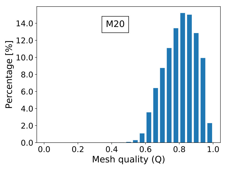 Figure 1
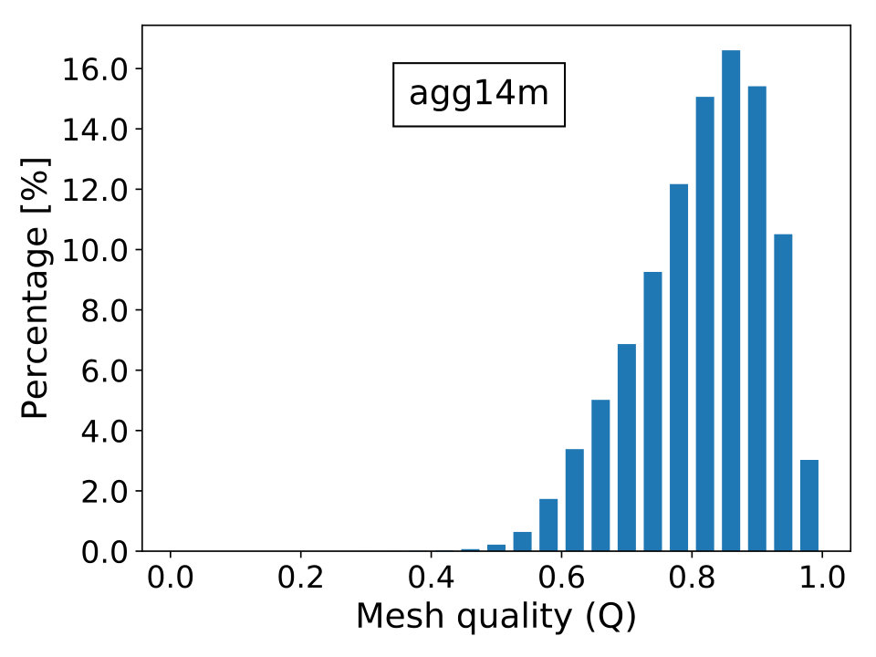 Figure 2
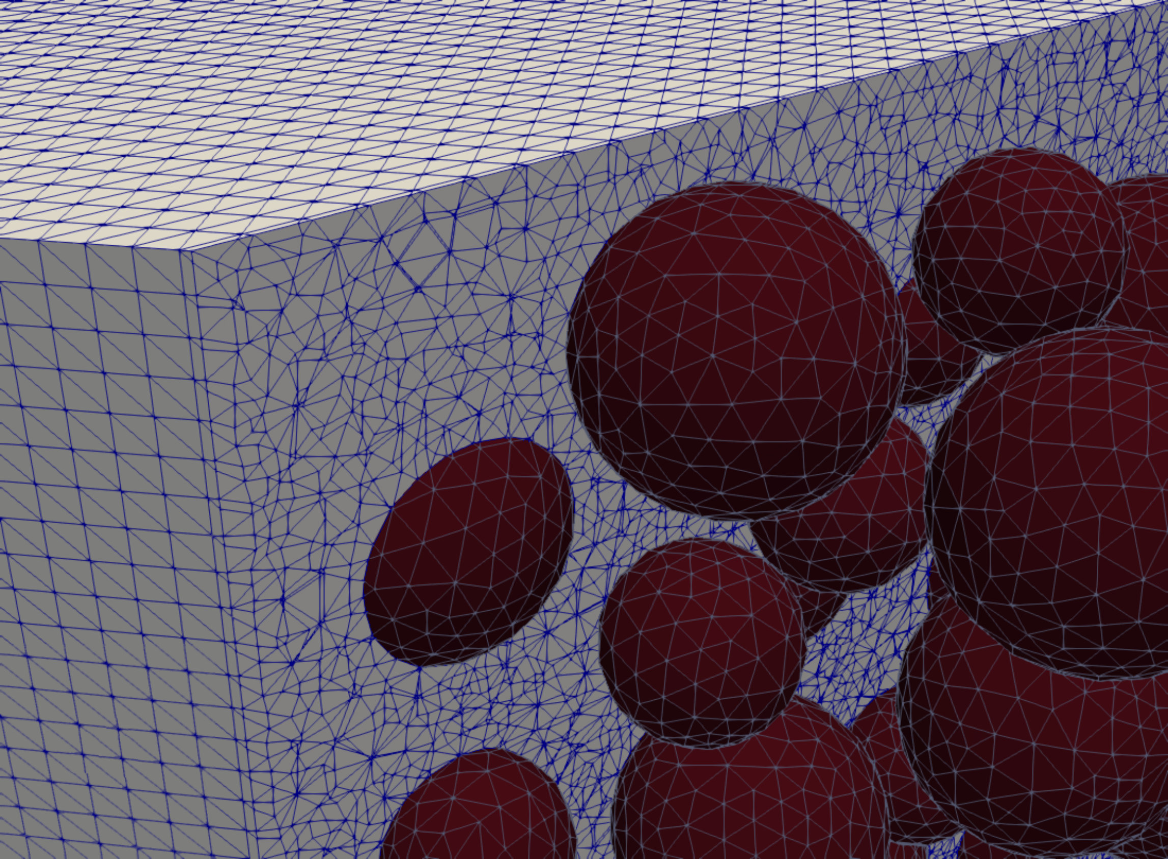 Figure 3
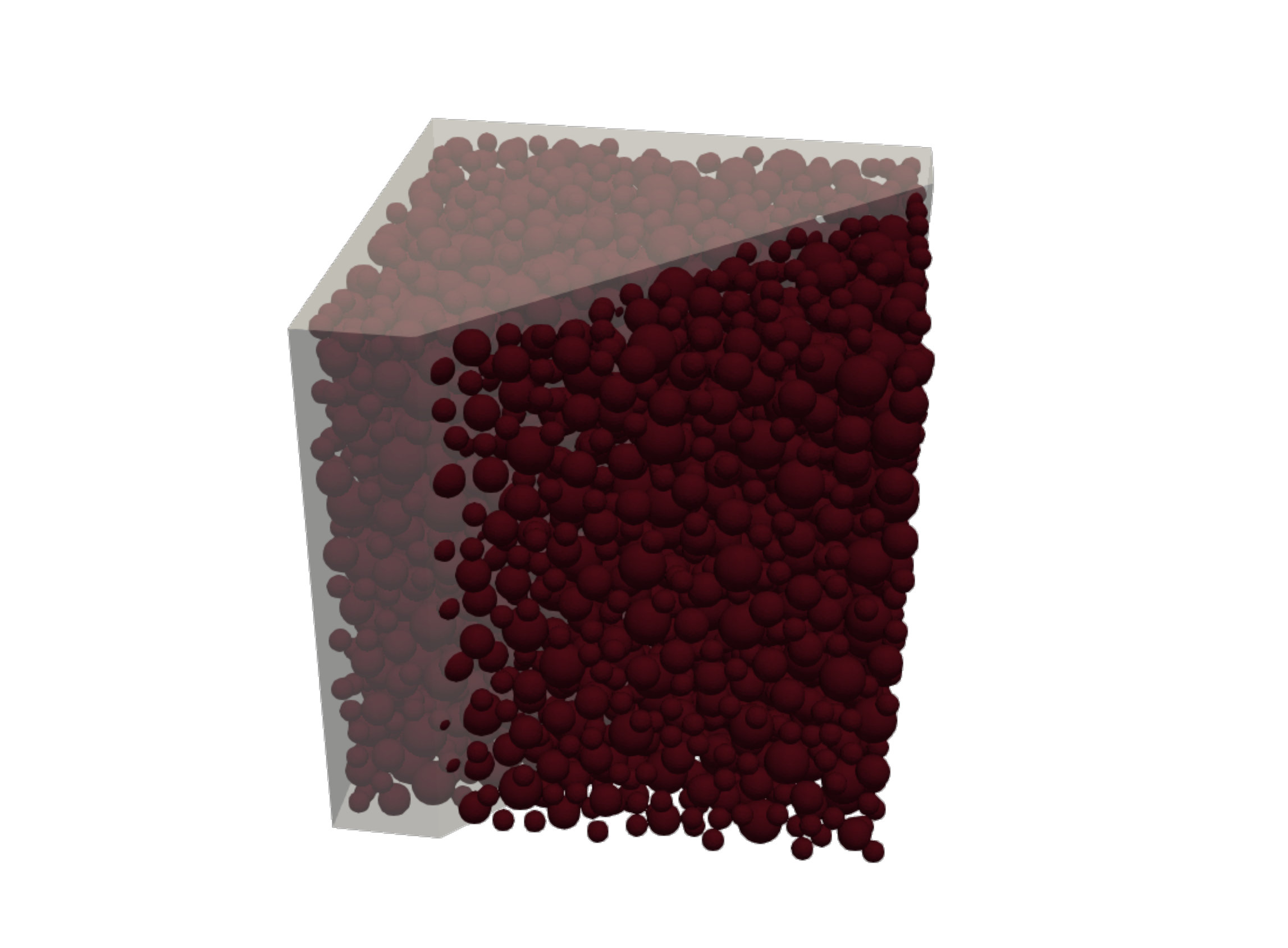 Figure 4
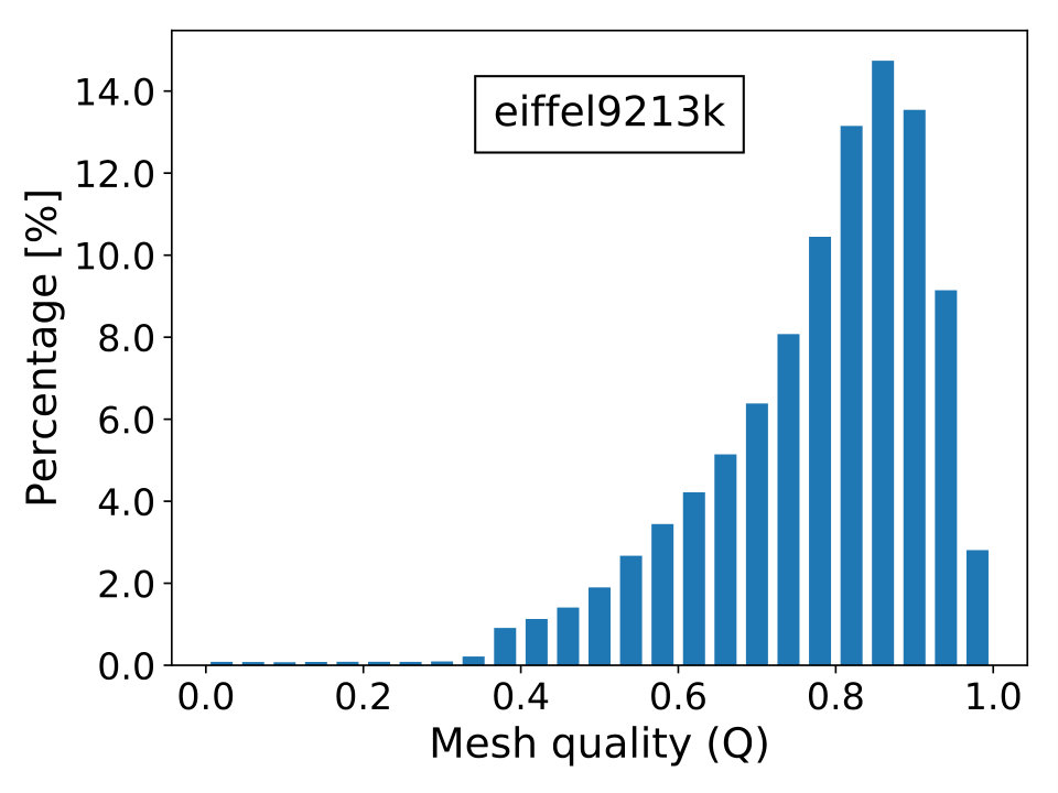 Figure 5
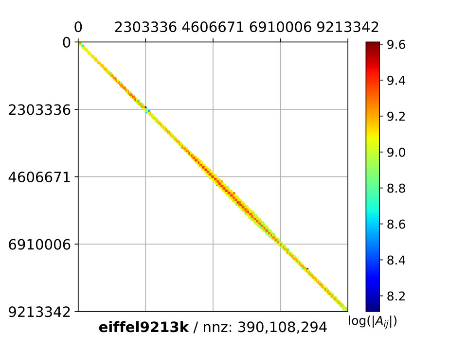 Figure 6
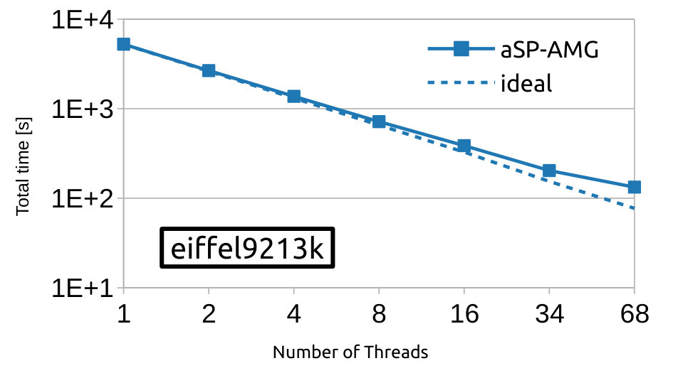 Figure 7
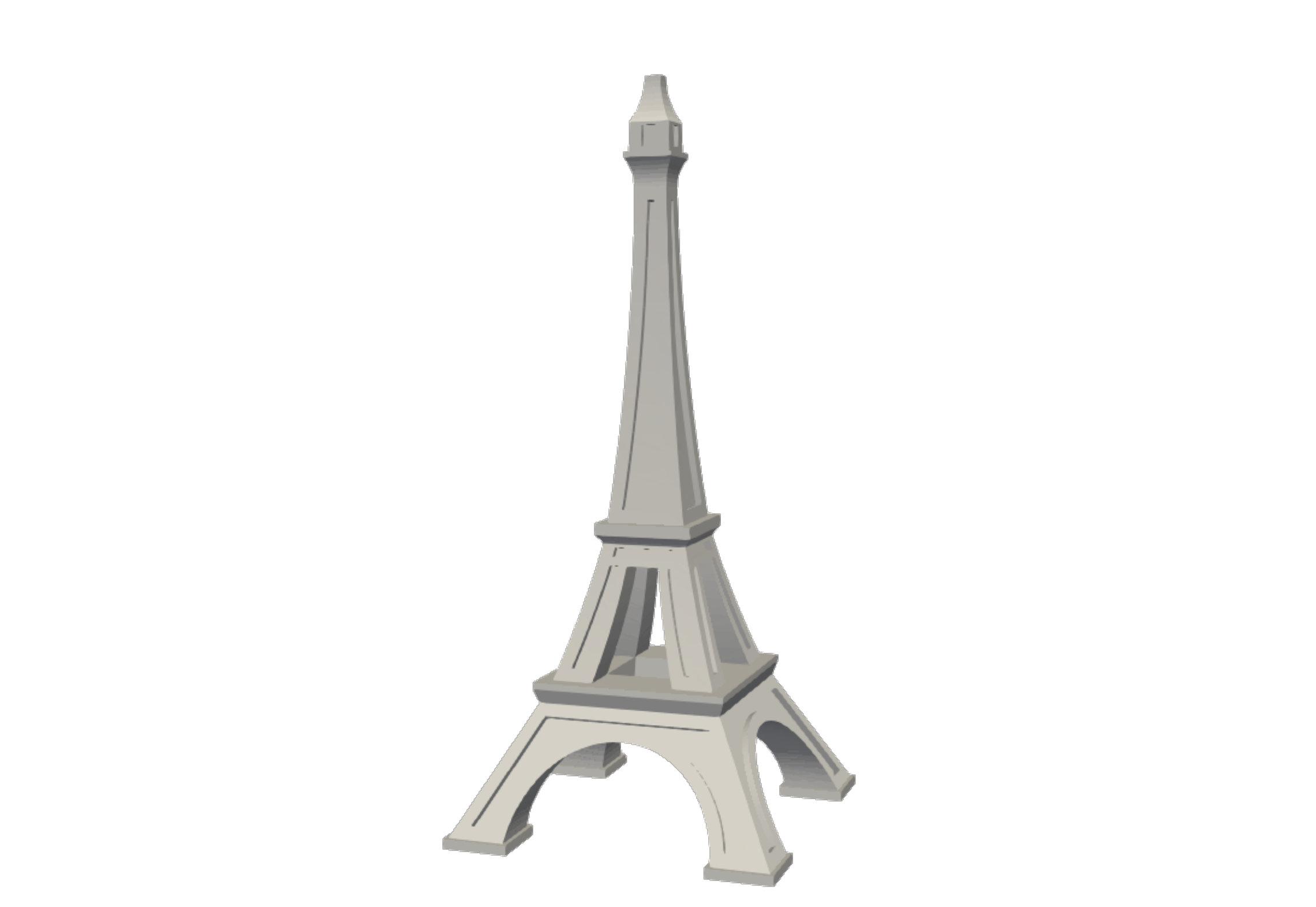 Figure 8
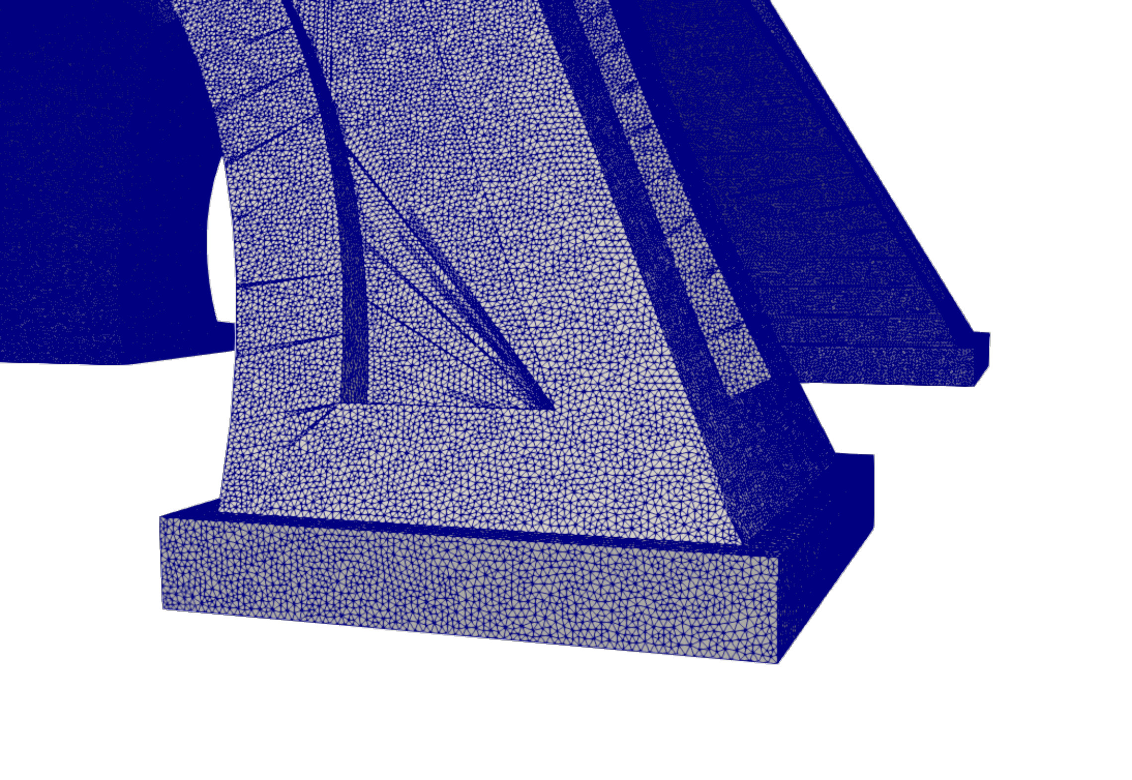 Figure 9
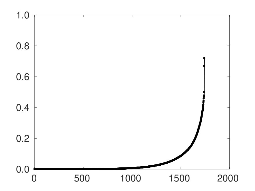 Figure 10
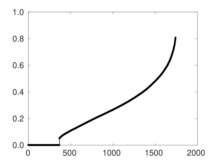 Figure 11
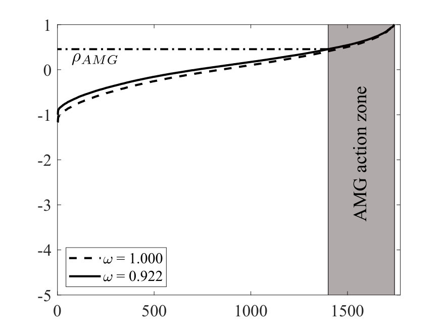 Figure 12
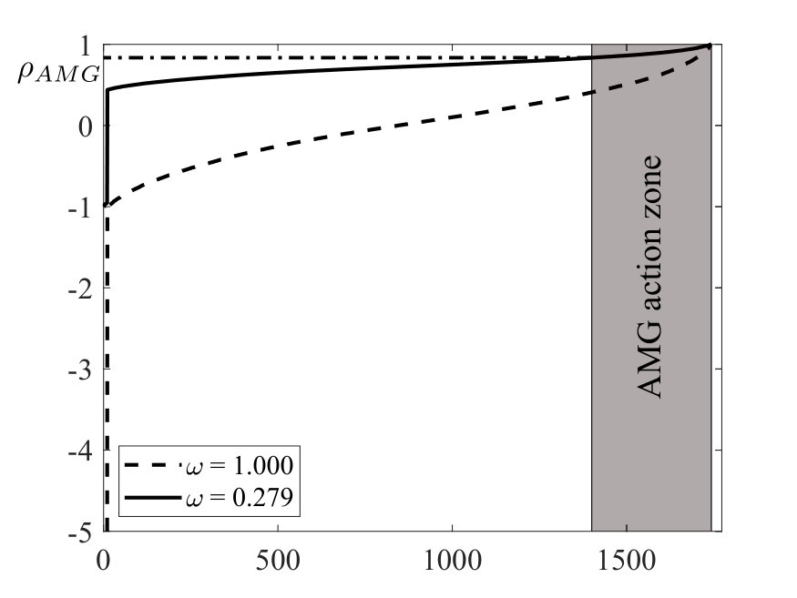 Figure 13
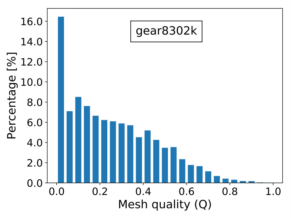 Figure 14
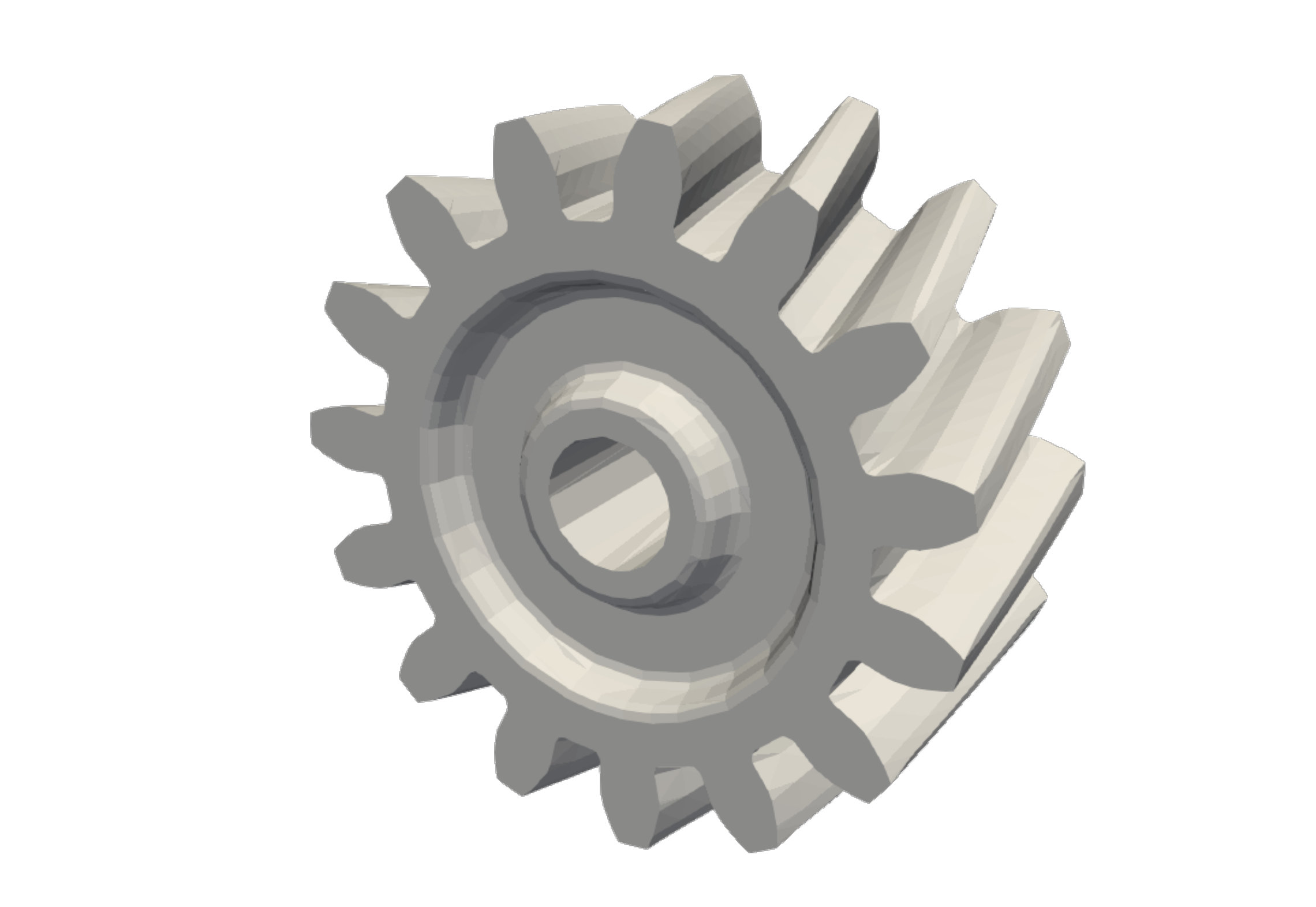 Figure 15
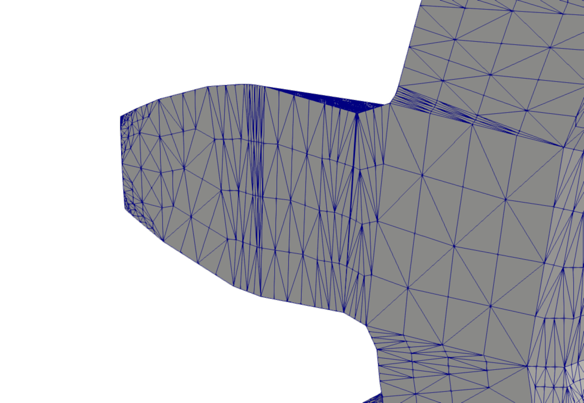 Figure 16
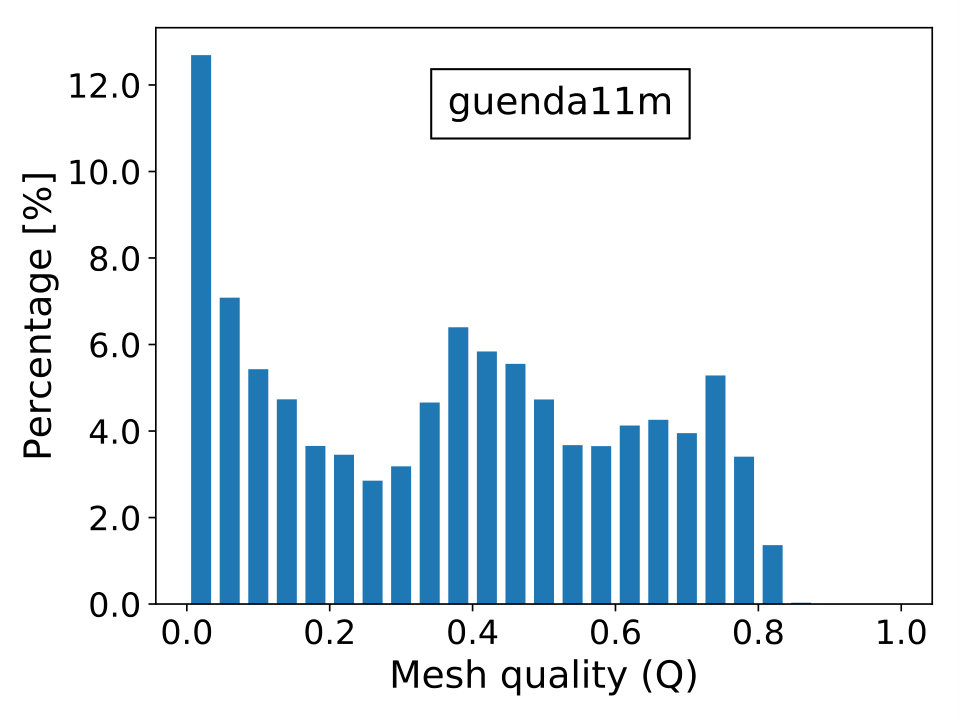 Figure 17
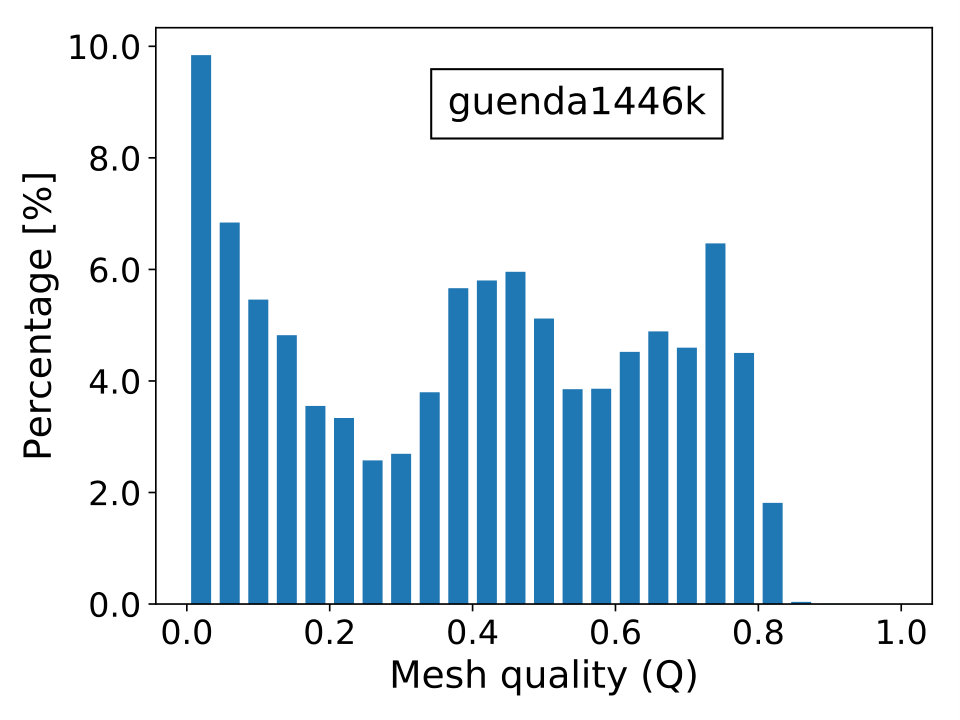 Figure 18
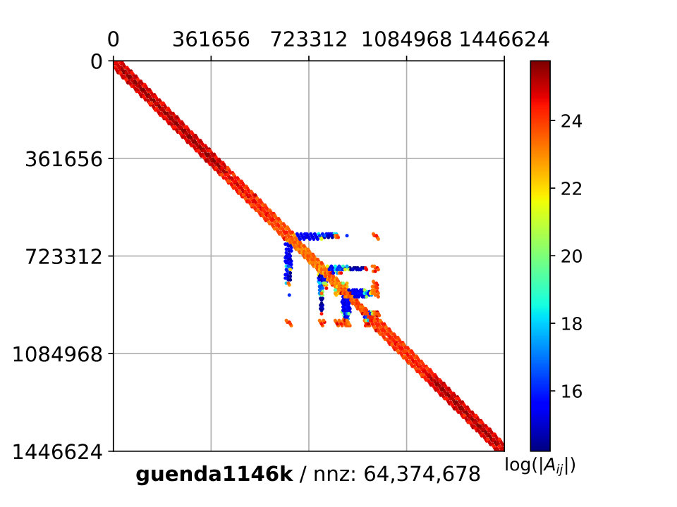 Figure 19
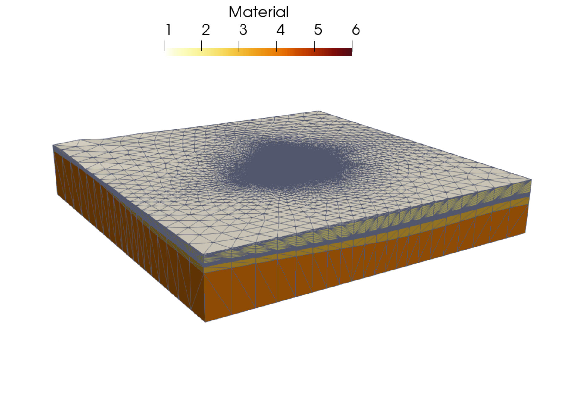 Figure 20
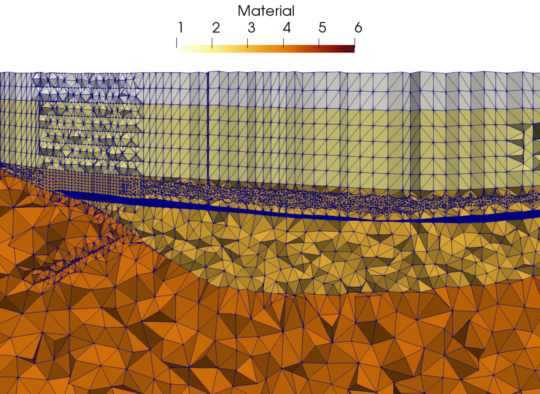 Figure 21
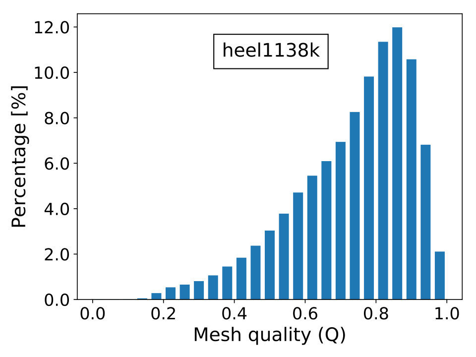 Figure 22
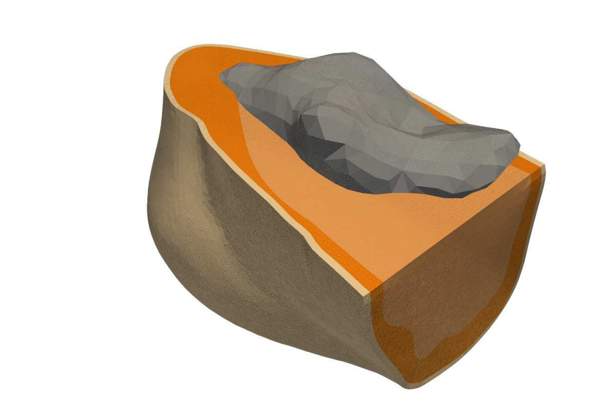 Figure 23
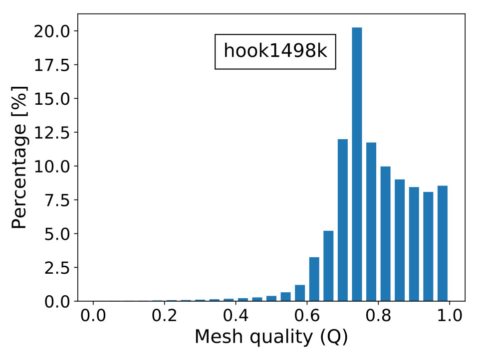 Figure 24
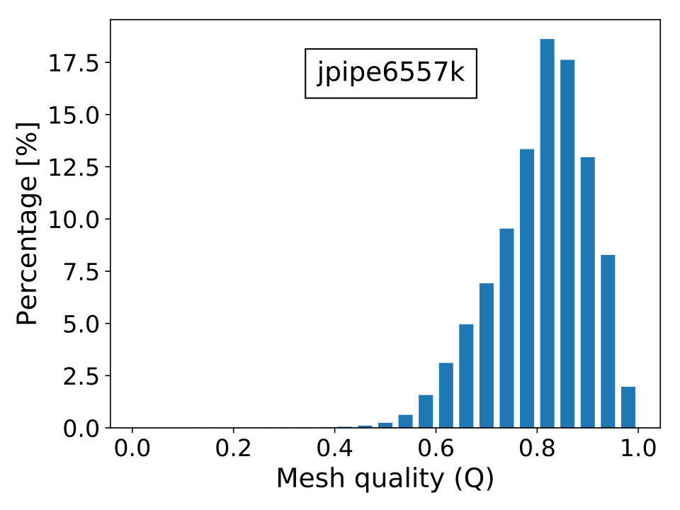 Figure 25
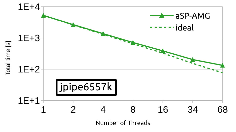 Figure 26
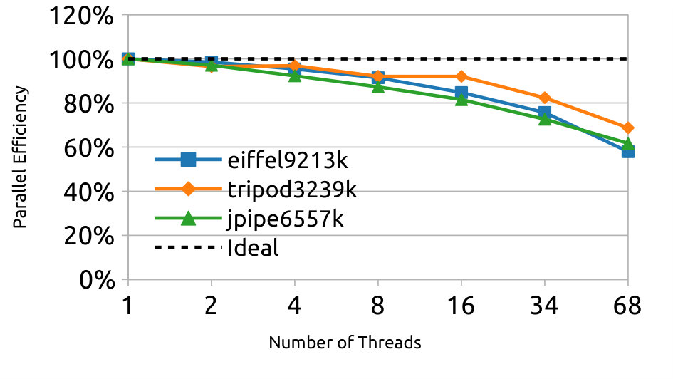 Figure 27
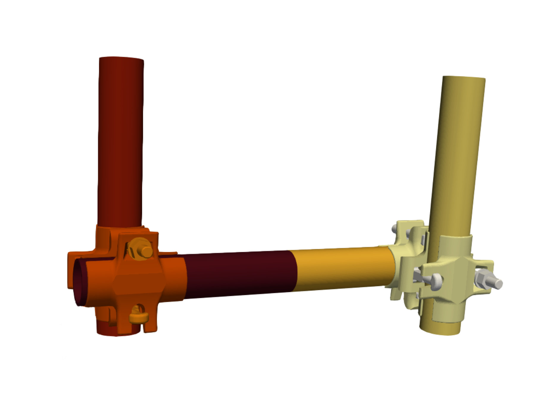 Figure 28
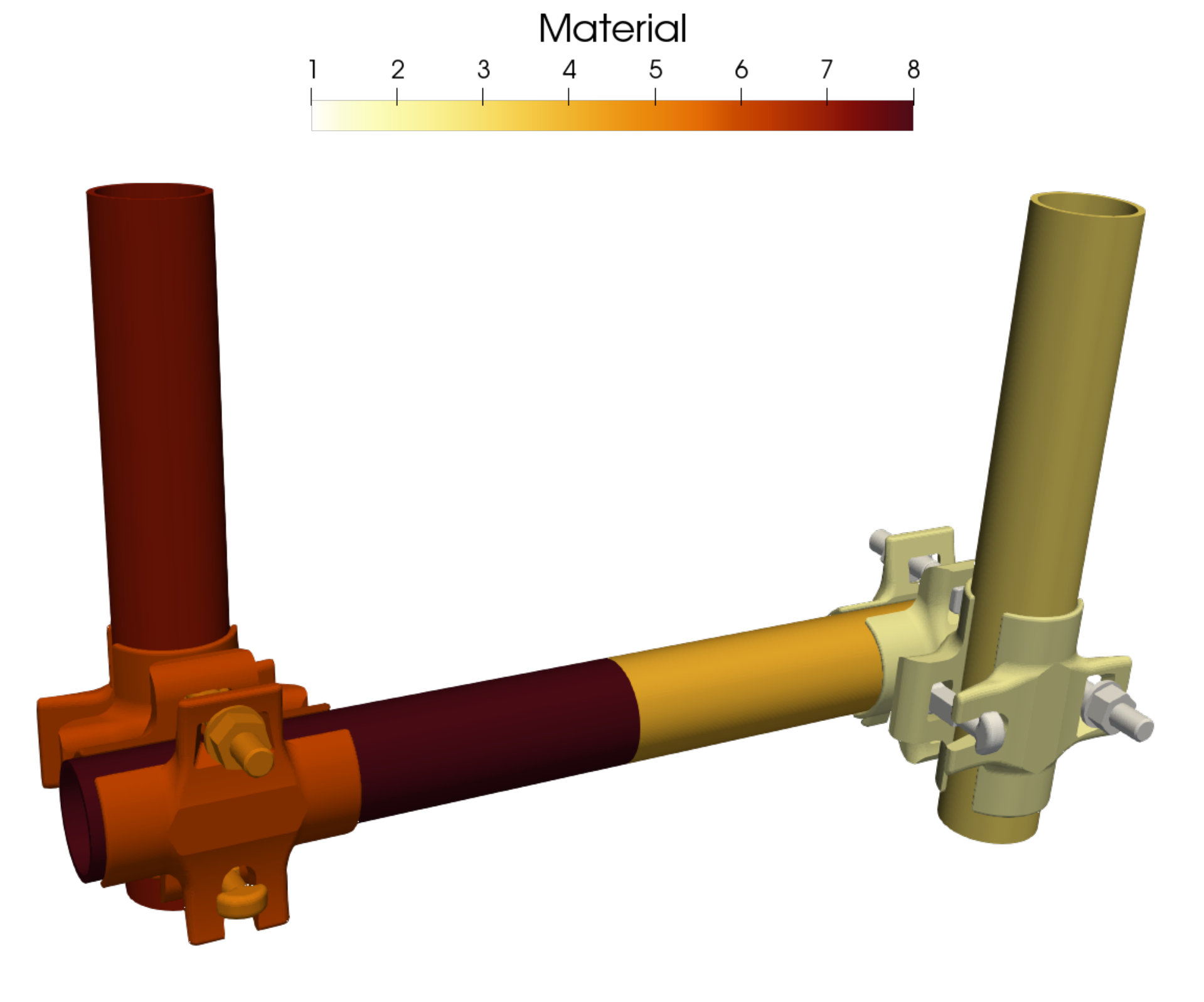 Figure 29
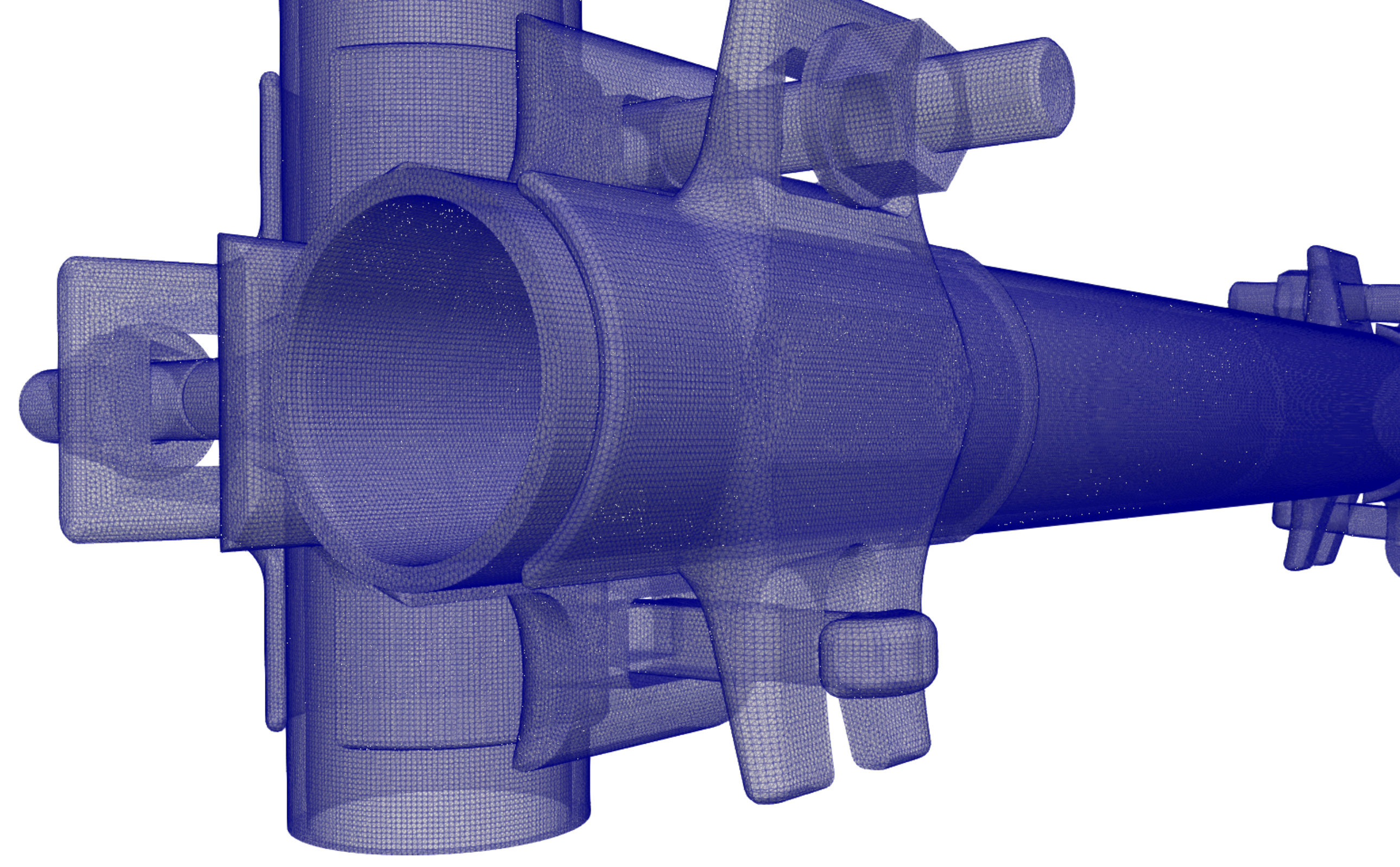 Figure 30
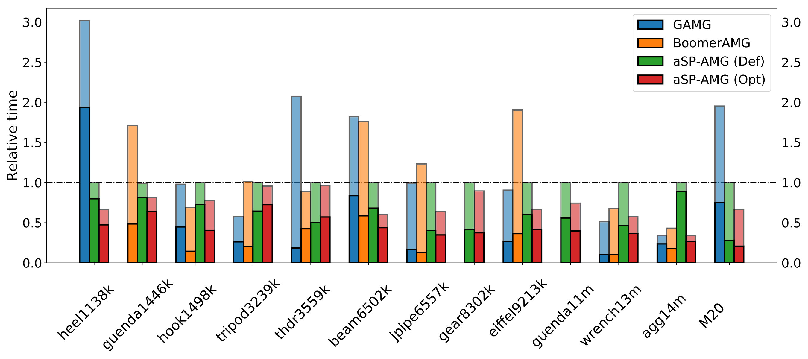 Figure 31
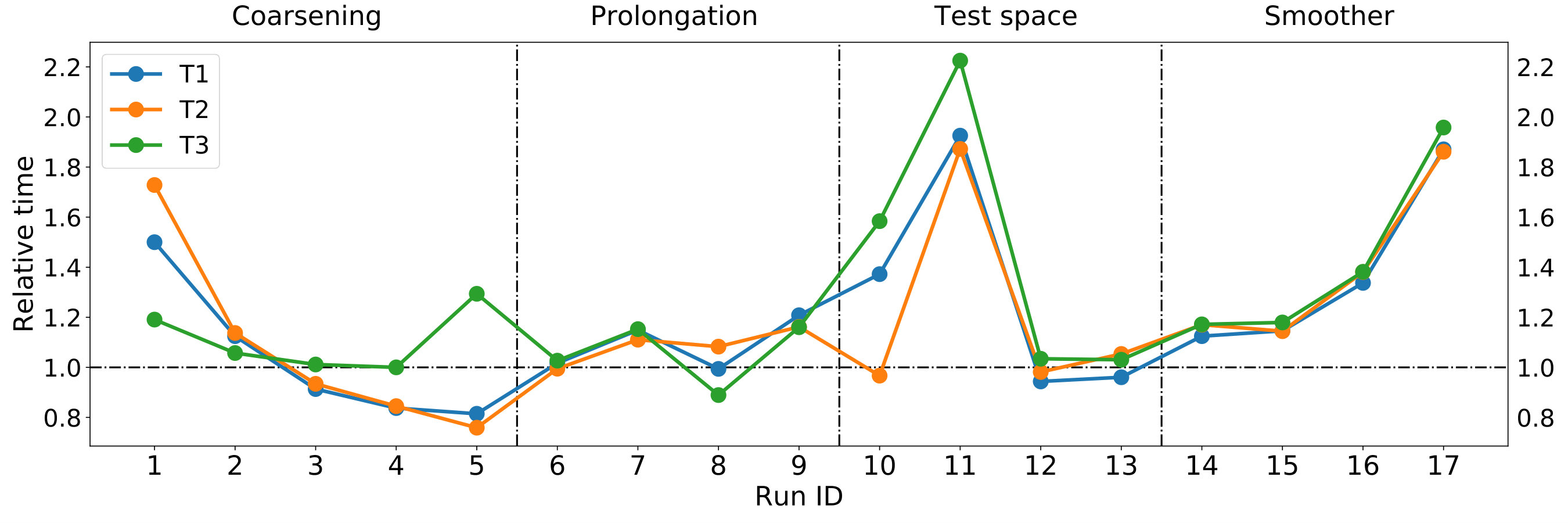 Figure 32
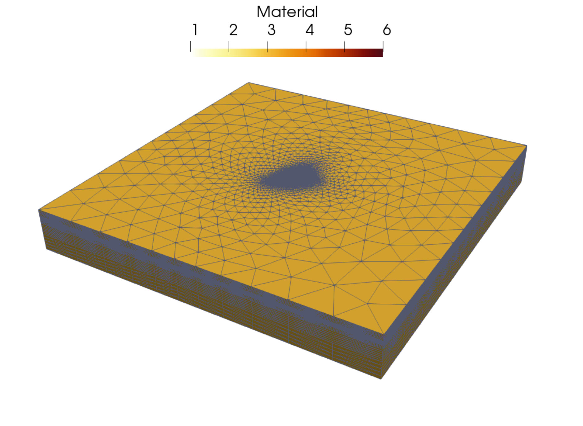 Figure 33
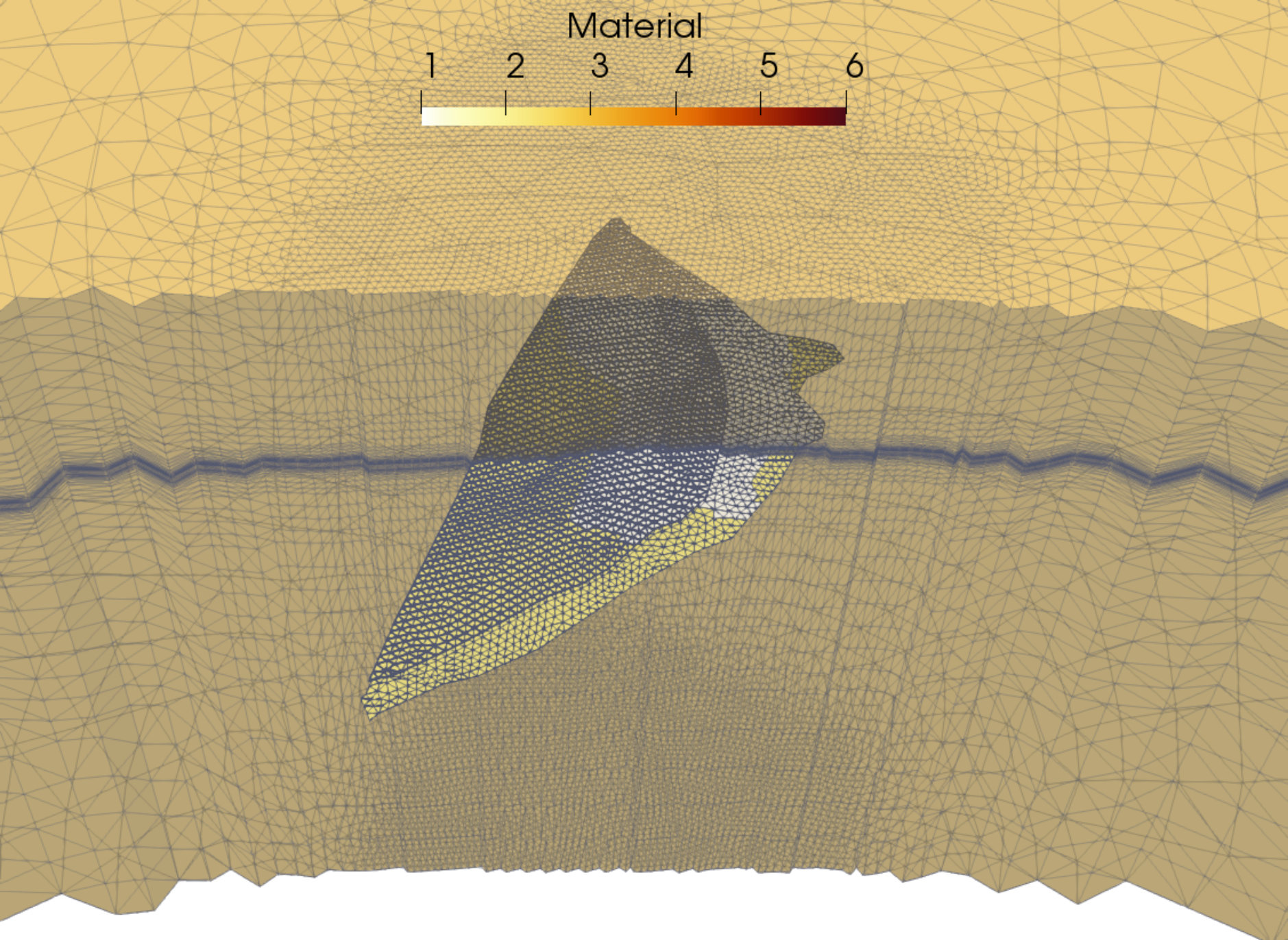 Figure 34
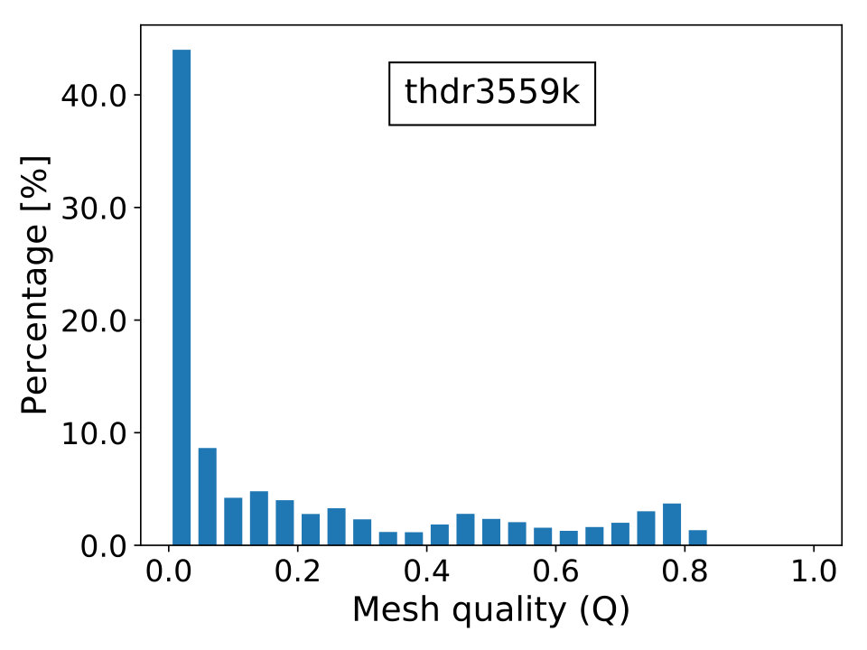 Figure 35
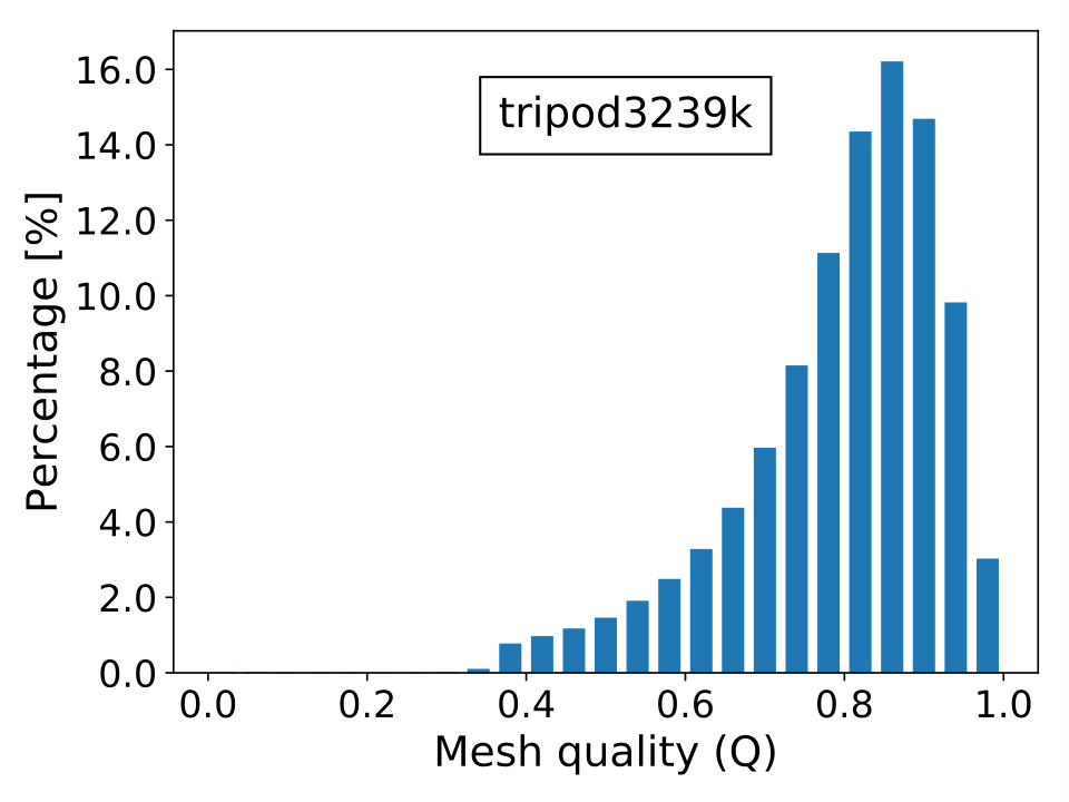 Figure 36
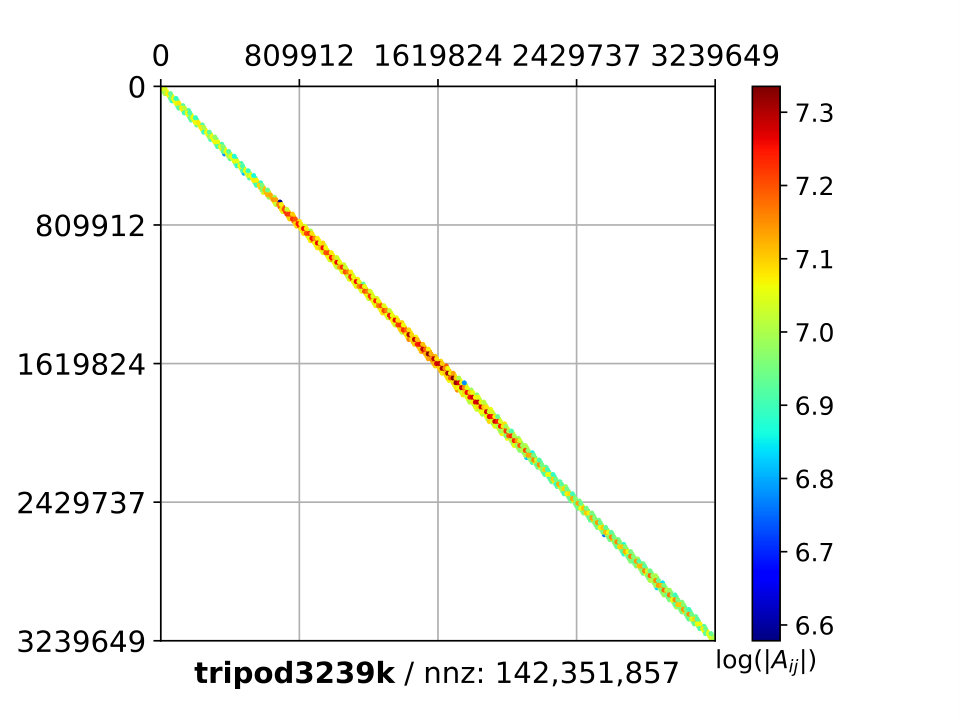 Figure 37
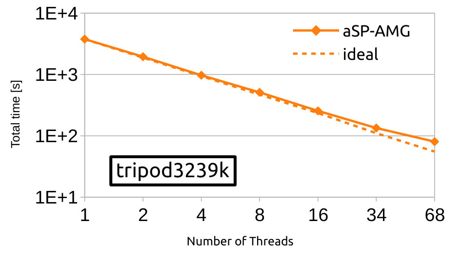 Figure 38
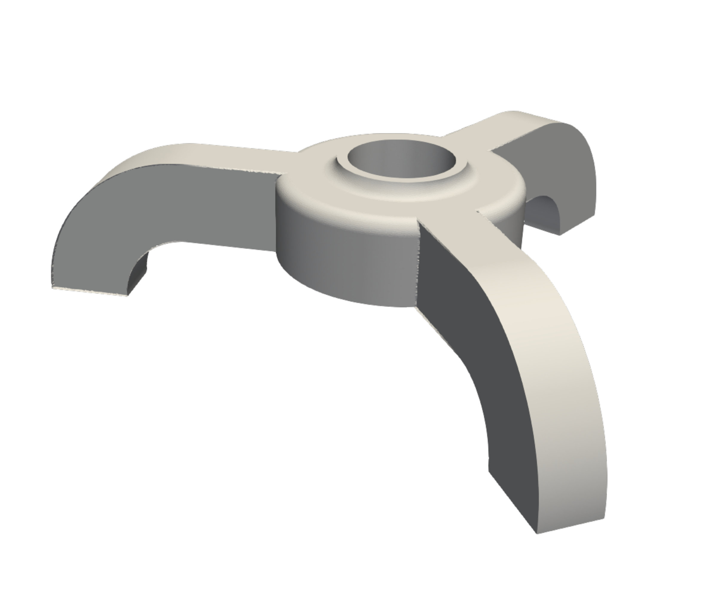 Figure 39
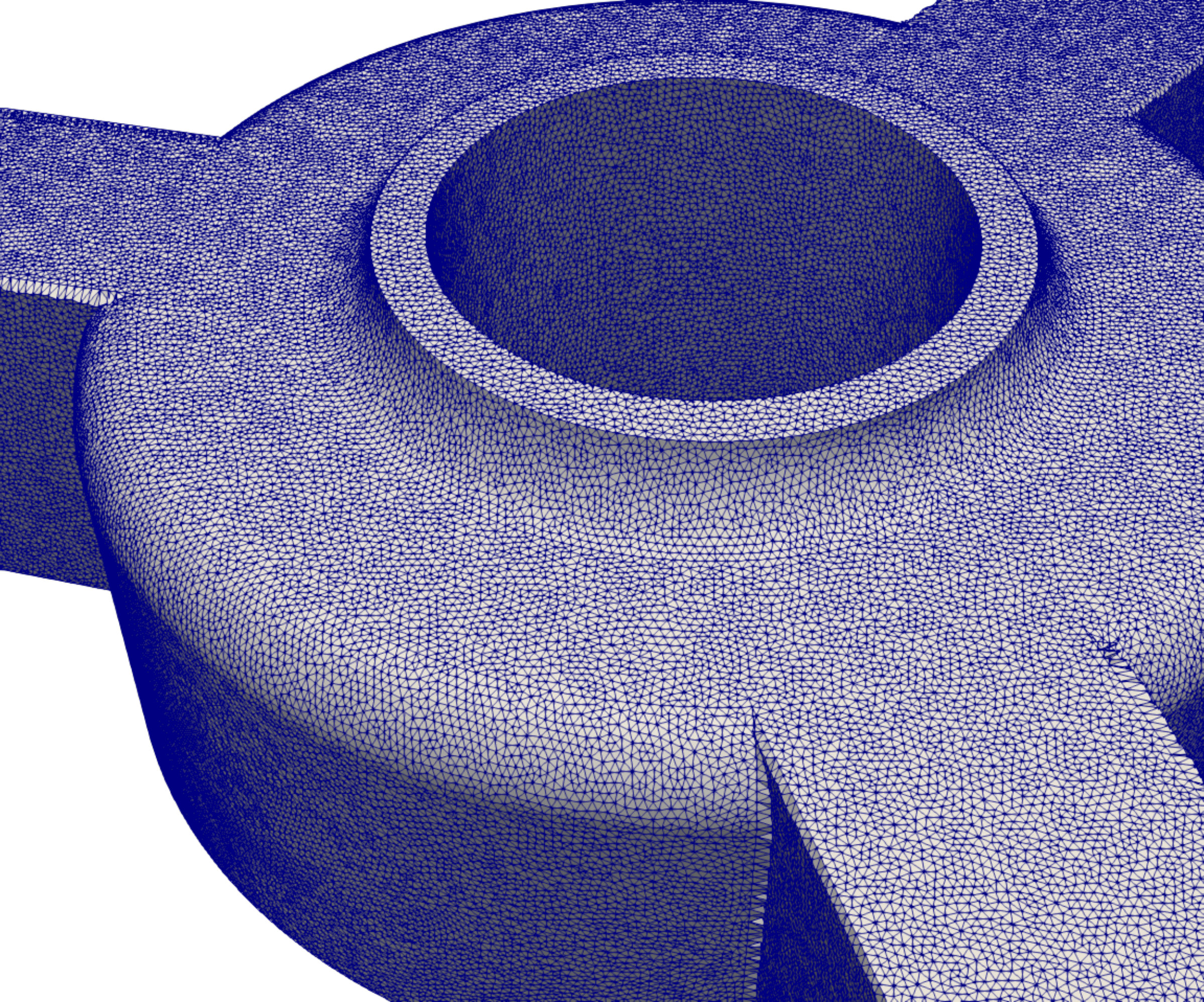 Figure 40
| Matrix name | FEM | Application | Description | Ill-conditioning | ||
| heel1138k | 1,138,443 | 51,677,937 | P1 | 3D Biomedicine | A.1 | MM |
| guenda1446k | 1,446,624 | 64,374,678 | P1 | 3D Geomechanics | A.2 | MM,DE |
| hook1498k | 1,498,023 | 59,374,451 | P1 | 3D Mechanical | A.3 | LC |
| tripod3239k | 3,239,649 | 142,351,857 | P1 | 3D Mechanical | A.4 | IM |
| thdr3559k | 3,559,398 | 81,240,330 | P1 | 3D Geomechanics | A.5 | MM,DE |
| beam6502k | 6,502,275 | 515,265,317 | Q1 | 3D Mechanical | A.6 | MM,LC |
| jpipe6557k | 6,557,808 | 335,451,702 | P1 | 3D Mechanical | A.7 | MM,LC |
| gear8302k | 8,302,032 | 672,580,800 | P2 | 3D Mechanical | A.8 | IM,DE |
| eiffel9213k | 9,213,342 | 390,108,294 | P1 | 3D Mechanical | A.9 | LC |
| guenda11m | 11,452,398 | 512,484,300 | P1 | 3D Geomechanics | A.2 | MM,DE |
| wrench13m | 12,995,364 | 589,759,812 | P1 | 3D Mechanical | A.10 | IM,LC |
| agg14m | 14,106,408 | 633,142,730 | P1 | 3D Mesoscale | A.11 | MM |
| M20 | 20,056,050 | 1,634,926,088 | P2 | 3D Mechanical | A.12 | DE,LC |
| Phase | Param. | Value |
| Smoother | ||
| Test Space | ||
| Coarsening | ||
| Prolongation | ||
| Test case | Results | |||||||||||
|---|---|---|---|---|---|---|---|---|---|---|---|---|
| T1 | 1.39 | 3.08 | 0.53 | 228 | 18.4 | 9.5 | 6.8 | 3.8 | 2.4 | 42.4 | 23.4 | 65.8 |
| T2 | 1.38 | 2.75 | 0.55 | 239 | 49.3 | 25.1 | 33.5 | 8.4 | 4.6 | 123.0 | 82.4 | 205.4 |
| T3 | 1.48 | 2.44 | 0.57 | 81 | 9.2 | 4.2 | 3.8 | 1.8 | 1.4 | 21.4 | 4.5 | 26.2 |
| Test case | Run ID | Param. | Results | |||||||||||
|---|---|---|---|---|---|---|---|---|---|---|---|---|---|---|
| T1 | 1 | 2 | 1.66 | 4.54 | 0.64 | 316 | 22.0 | 13.2 | 9.3 | 3.7 | 2.9 | 53.1 | 44.9 | 98.7 |
| 2 | 4 | 1.45 | 3.57 | 0.56 | 248 | 19.5 | 10.3 | 7.6 | 4.1 | 2.9 | 45.6 | 28.0 | 74.0 | |
| 3 | 6 | 1.34 | 2.79 | 0.51 | 224 | 17.4 | 8.4 | 6.2 | 3.6 | 2.3 | 39.0 | 20.7 | 60.1 | |
| 4 | 8 | 1.26 | 2.39 | 0.49 | 222 | 16.3 | 7.4 | 5.6 | 3.7 | 1.9 | 36.2 | 18.6 | 55.1 | |
| 5 | 10 | 1.21 | 2.11 | 0.47 | 229 | 15.5 | 7.0 | 5.3 | 4.2 | 1.5 | 35.1 | 18.2 | 53.6 | |
| T2 | 1 | 2 | 1.66 | 4.07 | 0.66 | 379 | 60.7 | 34.5 | 44.0 | 7.7 | 6.5 | 156.8 | 197.2 | 355.0 |
| 2 | 4 | 1.44 | 3.10 | 0.58 | 260 | 53.0 | 27.1 | 35.8 | 8.0 | 5.4 | 131.7 | 101.2 | 233.6 | |
| 3 | 6 | 1.33 | 2.49 | 0.53 | 228 | 48.5 | 22.9 | 31.8 | 8.2 | 4.2 | 117.8 | 73.5 | 191.9 | |
| 4 | 8 | 1.26 | 2.17 | 0.50 | 221 | 44.0 | 20.1 | 29.4 | 8.6 | 3.6 | 108.0 | 64.9 | 173.6 | |
| 5 | 10 | 1.20 | 1.92 | 0.48 | 210 | 41.2 | 18.4 | 27.8 | 9.2 | 3.2 | 101.8 | 53.6 | 155.9 | |
| T3 | 1 | 2 | 1.71 | 3.01 | 0.65 | 99 | 10.8 | 5.1 | 4.5 | 1.5 | 1.4 | 24.7 | 6.2 | 31.2 |
| 2 | 4 | 1.52 | 2.61 | 0.58 | 86 | 9.6 | 4.5 | 4.0 | 1.7 | 1.8 | 22.8 | 4.7 | 27.7 | |
| 3 | 6 | 1.45 | 2.34 | 0.55 | 91 | 9.1 | 3.9 | 4.1 | 1.8 | 1.5 | 21.8 | 4.6 | 26.5 | |
| 4 | 8 | 1.38 | 2.18 | 0.52 | 108 | 8.8 | 3.9 | 3.6 | 2.1 | 1.5 | 20.8 | 5.2 | 26.2 | |
| 5 | 10 | 1.29 | 2.04 | 0.49 | 375 | 7.8 | 3.7 | 3.3 | 2.1 | 1.4 | 19.2 | 14.5 | 33.9 | |
| Test case | Run ID | Param. | Results | ||||||||||||
|---|---|---|---|---|---|---|---|---|---|---|---|---|---|---|---|
| T1 | 6 | 2 | 50 | 1.39 | 3.15 | 0.53 | 229 | 18.2 | 9.4 | 6.9 | 3.8 | 2.6 | 42.5 | 23.9 | 66.9 |
| 7 | 10 | 50 | 1.39 | 3.79 | 0.53 | 236 | 18.9 | 11.3 | 7.6 | 5.4 | 3.3 | 48.0 | 27.3 | 75.6 | |
| 8 | 10 | 10 | 1.39 | 2.47 | 0.53 | 298 | 17.4 | 7.9 | 6.1 | 3.3 | 1.7 | 38.0 | 27.0 | 65.4 | |
| 9 | 10 | 100 | 1.39 | 3.90 | 0.53 | 256 | 19.4 | 11.4 | 8.0 | 5.5 | 3.2 | 49.3 | 29.9 | 79.5 | |
| T2 | 6 | 2 | 50 | 1.38 | 2.73 | 0.55 | 235 | 49.1 | 24.4 | 33.8 | 8.5 | 4.7 | 122.6 | 81.0 | 204.3 |
| 7 | 10 | 50 | 1.38 | 3.17 | 0.55 | 244 | 50.6 | 27.6 | 35.5 | 10.9 | 5.7 | 132.7 | 94.6 | 228.1 | |
| 8 | 10 | 10 | 1.38 | 1.95 | 0.55 | 419 | 45.8 | 19.9 | 30.7 | 6.4 | 2.3 | 107.0 | 114.8 | 222.4 | |
| 9 | 10 | 100 | 1.38 | 3.23 | 0.55 | 256 | 52.0 | 28.0 | 35.5 | 11.7 | 5.9 | 135.6 | 102.3 | 238.6 | |
| T3 | 6 | 2 | 50 | 1.48 | 2.49 | 0.56 | 82 | 9.5 | 4.2 | 3.8 | 2.0 | 1.6 | 22.3 | 4.3 | 26.9 |
| 7 | 10 | 50 | 1.48 | 2.66 | 0.56 | 85 | 10.5 | 4.5 | 4.1 | 2.3 | 1.7 | 24.9 | 4.9 | 30.2 | |
| 8 | 10 | 10 | 1.48 | 1.67 | 0.57 | 126 | 8.6 | 2.9 | 3.1 | 1.3 | 0.9 | 17.8 | 5.2 | 23.3 | |
| 9 | 10 | 100 | 1.48 | 2.82 | 0.56 | 91 | 9.7 | 4.8 | 4.2 | 2.4 | 1.9 | 24.6 | 5.4 | 30.4 | |
| Test case | Run ID | Param. | Results | ||||||||||||
|---|---|---|---|---|---|---|---|---|---|---|---|---|---|---|---|
| T1 | 10 | 20 | 10 | 1.37 | 3.09 | 0.53 | 223 | 43.7 | 9.1 | 6.6 | 3.7 | 2.7 | 67.1 | 22.9 | 90.3 |
| 11 | 30 | 10 | 1.37 | 2.99 | 0.53 | 235 | 79.9 | 9.5 | 6.6 | 4.0 | 2.5 | 103.7 | 22.7 | 126.7 | |
| 12 | 10 | 20 | 1.39 | 2.74 | 0.53 | 185 | 22.5 | 8.7 | 6.6 | 3.2 | 1.9 | 44.2 | 17.6 | 62.1 | |
| 13 | 10 | 30 | 1.39 | 2.51 | 0.53 | 182 | 26.0 | 8.0 | 6.2 | 2.8 | 2.0 | 46.4 | 16.6 | 63.2 | |
| T2 | 10 | 20 | 10 | 1.38 | 2.36 | 0.55 | 240 | 57.7 | 22.3 | 32.2 | 6.6 | 3.5 | 124.3 | 73.7 | 198.6 |
| 11 | 30 | 10 | 1.36 | 2.95 | 0.54 | 191 | 233.3 | 26.9 | 33.6 | 10.5 | 5.4 | 312.1 | 71.7 | 384.6 | |
| 12 | 10 | 20 | 1.38 | 2.38 | 0.55 | 240 | 59.0 | 22.2 | 32.9 | 7.2 | 3.7 | 127.2 | 73.9 | 201.6 | |
| 13 | 10 | 30 | 1.38 | 2.15 | 0.55 | 282 | 68.2 | 21.6 | 32.6 | 6.0 | 3.2 | 133.8 | 82.0 | 216.4 | |
| T3 | 10 | 20 | 10 | 1.49 | 2.80 | 0.57 | 76 | 22.9 | 4.6 | 4.0 | 2.4 | 2.1 | 37.0 | 4.2 | 41.5 |
| 11 | 30 | 10 | 1.49 | 2.77 | 0.57 | 74 | 40.7 | 4.6 | 3.7 | 2.4 | 1.8 | 54.2 | 3.9 | 58.3 | |
| 12 | 10 | 20 | 1.48 | 2.24 | 0.57 | 77 | 11.5 | 3.9 | 3.7 | 1.6 | 1.3 | 23.0 | 3.8 | 27.1 | |
| 13 | 10 | 30 | 1.48 | 2.15 | 0.57 | 85 | 13.1 | 3.5 | 3.3 | 1.4 | 1.0 | 23.1 | 3.7 | 27.0 | |
| Test case | Run ID | Param. | Results | |||||||||||||
|---|---|---|---|---|---|---|---|---|---|---|---|---|---|---|---|---|
| T1 | 14 | 4 | 8 | 1.39 | 3.04 | 1.04 | 187 | 20.7 | 9.2 | 13.8 | 3.4 | 2.3 | 51.1 | 22.4 | 74.0 | |
| 15 | 4 | 8 | 1.39 | 3.02 | 1.04 | 190 | 21.0 | 9.3 | 14.4 | 3.5 | 2.2 | 51.8 | 23.0 | 75.4 | ||
| 16 | 8 | 4 | 1.39 | 3.05 | 1.04 | 189 | 20.6 | 9.4 | 27.2 | 3.5 | 2.2 | 64.5 | 23.0 | 88.0 | ||
| 17 | 8 | 8 | 1.39 | 2.87 | 2.04 | 149 | 25.2 | 9.0 | 56.7 | 3.3 | 2.1 | 98.2 | 24.4 | 123.1 | ||
| T2 | 14 | 4 | 8 | 1.38 | 2.63 | 1.07 | 207 | 57.1 | 23.7 | 53.3 | 7.7 | 4.0 | 148.6 | 91.1 | 240.4 | |
| 15 | 4 | 8 | 1.38 | 2.62 | 1.07 | 196 | 55.3 | 24.1 | 53.2 | 7.6 | 4.0 | 147.6 | 86.7 | 235.1 | ||
| 16 | 8 | 4 | 1.38 | 2.61 | 1.06 | 197 | 55.0 | 24.2 | 102.1 | 7.5 | 4.3 | 195.7 | 87.1 | 283.6 | ||
| 17 | 8 | 8 | 1.38 | 2.48 | 2.08 | 199 | 82.6 | 40.4 | 110.6 | 6.3 | 7.0 | 250.8 | 131.1 | 382.3 | ||
| T3 | 14 | 4 | 8 | 1.49 | 2.31 | 1.10 | 79 | 10.6 | 3.7 | 6.9 | 1.7 | 1.5 | 25.6 | 4.7 | 30.7 | |
| 15 | 4 | 8 | 1.49 | 2.33 | 1.11 | 79 | 10.5 | 3.9 | 7.1 | 1.6 | 1.6 | 25.8 | 4.8 | 30.9 | ||
| 16 | 8 | 4 | 1.48 | 2.28 | 1.07 | 69 | 10.8 | 4.0 | 13.2 | 1.6 | 1.3 | 31.9 | 4.1 | 36.2 | ||
| 17 | 8 | 8 | 1.48 | 2.24 | 2.10 | 66 | 12.6 | 3.6 | 26.8 | 1.5 | 1.2 | 46.5 | 4.6 | 51.3 | ||
| Test case | Preconditioner | ||||||
| heel1138k | GAMG | 1.08 | 1.48 | 84 | 75.8 | 42.3 | 118.1 |
| BoomerAMG | 1.47 | 2.73 | — | — | — | ||
| aSP-AMG (Def) | 1.39 | 3.29 | 82 | 31.2 | 7.9 | 39.1 | |
| aSP-AMG (Opt) | 1.17 | 1.98 | 103 | 18.5 | 7.5 | 26.0 | |
| guenda1446k | GAMG | 1.10 | 1.70 | — | — | — | |
| BoomerAMG | 1.69 | 2.06 | 239 | 12.7 | 32.1 | 44.8 | |
| aSP-AMG (Def) | 1.48 | 2.44 | 81 | 21.4 | 4.5 | 26.2 | |
| aSP-AMG (Opt) | 1.38 | 1.88 | 113 | 16.7 | 4.6 | 21.3 | |
| hook1498k | GAMG | 1.11 | 1.92 | 128 | 13.6 | 16.2 | 29.8 |
| BoomerAMG | 1.61 | 2.02 | 154 | 4.4 | 16.5 | 20.9 | |
| aSP-AMG (Def) | 1.37 | 2.72 | 151 | 22.1 | 8.3 | 30.4 | |
| aSP-AMG (Opt) | 1.20 | 1.81 | 279 | 12.3 | 11.3 | 23.4 | |
| tripod3239k | GAMG | 1.09 | 1.56 | 77 | 17.2 | 20.7 | 38.2 |
| BoomerAMG | 1.52 | 3.04 | 181 | 13.3 | 53.1 | 66.4 | |
| aSP-AMG (Def) | 1.39 | 3.08 | 228 | 42.4 | 23.4 | 65.8 | |
| aSP-AMG (Opt) | 1.26 | 1.94 | 172 | 47.7 | 15.2 | 62.9 | |
| thdr3559k | GAMG | 1.09 | 1.62 | 933 | 23.2 | 237.4 | 260.6 |
| BoomerAMG | 1.71 | 2.03 | 176 | 53.1 | 58.1 | 111.2 | |
| aSP-AMG (Def) | 1.46 | 2.34 | 416 | 62.7 | 62.9 | 125.6 | |
| aSP-AMG (Opt) | 1.70 | 2.18 | 136 | 71.7 | 49.3 | 121.6 | |
| beam6502k | GAMG | 1.05 | 1.16 | 42 | 141.1 | 165.9 | 307.0 |
| BoomerAMG | 1.26 | 1.35 | 81 | 98.8 | 198.2 | 297.0 | |
| aSP-AMG (Def) | 1.41 | 2.36 | 87 | 115.1 | 53.6 | 168.7 | |
| aSP-AMG (Opt) | 1.19 | 1.46 | 83 | 73.8 | 28.0 | 101.8 |
| Test case | Preconditioner | ||||||
| jpipe6557k | GAMG | 1.09 | 1.45 | 262 | 40.1 | 195.4 | 235.5 |
| BoomerAMG | 1.53 | 2.61 | 358 | 30.9 | 261.1 | 292.0 | |
| aSP-AMG (Def) | 1.41 | 2.42 | 518 | 95.4 | 141.5 | 236.9 | |
| aSP-AMG (Opt) | 1.20 | 1.55 | 407 | 82.3 | 69.2 | 151.5 | |
| gear8302k | GAMG | 1.03 | 1.17 | — | — | — | |
| BoomerAMG | 1.61 | 2.09 | — | — | — | ||
| aSP-AMG (Def) | 1.38 | 2.04 | 652 | 412.6 | 586.9 | 999.5 | |
| aSP-AMG (Opt) | 1.23 | 1.65 | 628 | 374.0 | 521.1 | 895.1 | |
| eiffel9213k | GAMG | 1.09 | 1.64 | 167 | 55.1 | 131.1 | 186.2 |
| BoomerAMG | 1.49 | 2.85 | 376 | 74.6 | 316.2 | 390.8 | |
| aSP-AMG (Def) | 1.38 | 2.75 | 239 | 123.0 | 82.4 | 205.4 | |
| aSP-AMG (Opt) | 1.17 | 1.72 | 214 | 86.1 | 49.9 | 136.0 | |
| guenda11m | GAMG | 1.08 | 1.59 | — | — | — | |
| BoomerAMG | 1.70 | 2.22 | — | — | — | ||
| aSP-AMG (Def) | 1.49 | 2.27 | 374 | 596.6 | 471.9 | 1068.5 | |
| aSP-AMG (Opt) | 1.44 | 2.02 | 436 | 424.1 | 371.4 | 795.5 | |
| wrench13m | GAMG | 1.08 | 1.52 | 139 | 41.8 | 162.2 | 204.0 |
| BoomerAMG | 1.51 | 2.98 | 183 | 40.5 | 227.9 | 268.4 | |
| aSP-AMG (Def) | 1.39 | 3.12 | 326 | 183.8 | 215.2 | 399.0 | |
| aSP-AMG (Opt) | 1.17 | 1.70 | 211 | 146.2 | 82.6 | 228.8 | |
| agg14m | GAMG | 1.08 | 1.59 | 30 | 82.1 | 37.8 | 119.9 |
| BoomerAMG | 1.55 | 1.84 | 89 | 61.9 | 88.7 | 150.6 | |
| aSP-AMG (Def) | 1.42 | 3.73 | 29 | 310.8 | 37.7 | 348.5 | |
| aSP-AMG (Opt) | 1.18 | 1.70 | 64 | 93.8 | 24.5 | 118.3 | |
| M20 | GAMG | 1.03 | 1.16 | 113 | 1274.7 | 2046.2 | 3320.9 |
| BoomerAMG | 1.54 | 1.58 | — | — | — | ||
| aSP-AMG (Def) | 1.38 | 2.26 | 401 | 473.6 | 1225.8 | 1699.4 | |
| aSP-AMG (Opt) | 1.14 | 1.44 | 350 | 353.2 | 779.4 | 1132.6 |
Peer Reviews
No public reviews on file for this paper yet. If you reviewed it on a platform where reviews are public (OpenReview, ICLR, NeurIPS, ICML), you can paste yours below so the community can read it here.
Videos
No videos yet. Explain this paper in a talk, walkthrough, or lecture? Add one.
A robust adaptive algebraic multigrid linear solver for structural mechanics
Andrea Franceschini
Victor A. Paludetto Magri
Gianluca Mazzucco
Nicolò Spiezia
Carlo Janna
Department of Energy Resources, Stanford University, Stanford, CA, United States of America
Department ICEA, University of Padova, Via Marzolo, 9 - 35131 Padova, Italy
M3E s.r.l., Via Giambellino, 7 - 35129 Padova, Italy
Abstract
The numerical simulation of structural mechanics applications via finite elements usually requires the solution of large-size and ill-conditioned linear systems, especially when accurate results are sought for derived variables interpolated with lower order functions, like stress or deformation fields. Such task represents the most time-consuming kernel in commercial simulators; thus, it is of significant interest the development of robust and efficient linear solvers for such applications. In this context, direct solvers, which are based on LU factorization techniques, are often used due to their robustness and easy setup; however, they can reach only superlinear complexity, in the best case, thus, have limited applicability depending on the problem size. On the other hand, iterative solvers based on algebraic multigrid (AMG) preconditioners can reach up to linear complexity for sufficiently regular problems but do not always converge and require more knowledge from the user for an efficient setup. In this work, we present an adaptive AMG method specifically designed to improve its usability and efficiency in the solution of structural problems. We show numerical results for several practical applications with millions of unknowns and compare our method with two state-of-the-art linear solvers proving its efficiency and robustness.
keywords:
AMG , linear solver , preconditioning , ill-conditioning , structural problems , parallel computing
††journal: Comp. Methods in Appl. Mech. and Eng.
1 Introduction
Across a broad range of structural mechanics applications, the demand for more accurate, complex and reliable numerical simulations is increasing exponentially. In this context, the Finite Element Method (FEM) remains the most widely used approach and the number of new extremely challenging applications is countless, e.g., modeling of fractal formation in macroscopic elasto-plasticity in three-dimensional bodies [1], simulation of cardiac mechanics [2], submarine landslides [3], stir welding processes [4], concrete gravity dam [5], just to name some recent applications. In all the problems mentioned above, the underlying partial differential equations (PDEs) are discretized to approximate the continuous solution in an algebraic system of equations of the form:
[TABLE]
with and , the right hand side and solution vectors, respectively, belonging to and the matrix deriving from the Finite Element discretization. For small strain mechanical problems, the linear system in (1) assumes the notation , where the vectors and represent the unknown nodal displacements and the applied nodal forces, respectively, and the matrix arises from the numerical integration of , where stands for the constitutive matrix and contains the spatial derivatives of the element shape functions . If the material is linear elastic, as assumed in this work, the matrix is Symmetric Positive Definite (SPD) and it is fully defined once the Young modulus and the Poisson ratio are assigned to each element composing the grid.
In numerical simulations, the solution of the linear system in (1) is the most time-consuming part of the entire process, taking up of the total computational time [6]. With the constant demand for larger simulations, involving up to billions of unknowns, the linear equation solver is the most significant bottleneck, and an inefficient algorithm may dramatically slow down the simulations process, forcing either to simplify the problem or to wait for a very long time for the results.
Linear equation solvers may be grouped into two broad categories: direct methods and iterative methods. The main advantages of direct methods are their generality and robustness. However, the matrix factors created to solve the system are often significantly denser than the original matrix. This issue leads to memory shortage for both forming and storing the factors, in particular for large-scale system arising from the discretization of three-dimensional problems. On the other hand, iterative methods are much more suitable for the solution of large systems of equations and hence are gaining more and more attention as far as the dimension of the computational grid increases. However, iterative methods do not guarantee the convergence to the scheme, unless a proper preconditioner is adopted. In fact, preconditioning the system is essential not only to accelerate the convergence rate, but also to avoid divergence in ill-conditioned cases.
In linear elastic problems, as those investigated in this work, ill-conditioned systems may arise due to several conditions, such as the presence of multiple materials or highly distorted elements, two of the most common source of ill-conditioness in structural problems. The first one is when the model is characterized by materials with significantly different constitutive characteristics and therefore the entries of the linear system matrix present large jumps. This is the case for example when a soft and hard tissues are connected [7, 8, 9] or when a solid matrix presents soft inclusions [10, 11, 12, 13]. The second case appears when the model is characterized by a highly distorted mesh, with poorly proportioned elements. This is the case when complex geometries characterize the model, which cannot be discretized with a structured mesh. This undesired situation is becoming more frequent since it is increasingly common to create meshes directly from complex CAD solid geometries [14, 15] or from an X-Ray tomography [16, 17, 18, 19]. Moreover, newly developed technologies, e.g., additive manufacturing, allow to create elaborated solids, with consequent demanding numerical simulations [20, 21, 22]. Besides, also the presence of materials close to the incompressibility limit or a loosely constrained body can lead to an ill-conditioned system. In the last decades, several types of preconditioners have been developed, such as incomplete factorizations [23, 24, 25], sparse approximate inverses [26, 27, 28, 29], domain decomposition [30, 31, 32, 33] and Algebraic Multigrid (AMG) methods. This paper focuses on the last category.
AMG methods are built on a hierarchy of levels associated with linear problems of decreasing size. Such methods are defined by the choice of interpolation operators, which transfers information between different levels; the coarsening strategy, which guides the definition of new levels; the smoothing technique, which solves high frequencies components of the error on the given level and, lastly, the application strategy, which defines how the multigrid cycle is applied.
Several families of AMG methods can be found in the literature. The first multigrid strategy, namely the classical AMG [34, 35], was proposed in the early 1980s for the efficient solution of M-matrices and Poisson models. These methods are built on the knowledge that the near-kernel of the operator is well approximated by the constant vector, which is a limiting hypothesis in linear elasticity problems. In the latter, a larger near-kernel, usually well represented by the rigid body modes (RBMs), is needed to obtain good results. The first attempt to overcome such limitation came in the early 1990s with the Smoothed Aggregation AMG (SA-AMG) method, where coarsening is done via aggregation of nodes and interpolation is built column-wise starting from a tentative operator spanning the RBMs in the aggregates [36, 37]. The element-based AMG family is composed by the energy-minimization AMGe [38], element-free AMGe [39] and spectral AMGe [40]. Here, the coarse spaces are constructed via an energy minimization process with the aim of improving robustness by alleviating the heuristics based on M-matrices properties implemented in classical AMG. More recently, the adaptive and Bootstrap AMG (AMG and BAMG, respectively) were designed for the solution of more difficult problems where the classical and smoothed AMG may fail or show poor convergence [41, 42, 43, 44]. In such methods, no preliminary assumption is made about the near-null space of , but it is approximated adaptively during the AMG hierarchy construction. For a comprehensive review of algebraic multigrid variants, we refer the reader to Xu and Zikatanov [45].
In the context of elasticity problems, Yoo [46] presented a W-cycle method for solving linear elasticity problems in the nearly incompressible limit and Griebel et al. [47] presented a generalization of the classical AMG where a block interpolation method is proposed and showed to reproduce the RBMs components in a multilevel strategy. Baker et al. [48] investigated several approaches for improving convergence of classical AMG when solving linear elasticity problems by incorporating the RBMs in the range of interpolation.
This work presents an extension of the adaptive Smoothing and Prolongation based Algebraic Multigrid method (aSP-AMG), proposed by [49], with the aim of specifically improving its performance for the solution of linear elasticity problems. Such method follows the path of bootstrap and adaptive AMG which is to build an approximation of the near-null space components of the problem at hand automatically. Also, this method proposes new strategies for computing the interpolation operators in a least-squares sense and introduces the Adaptive Factorized Sparse Approximate Inverse (aFSAI) as a flexible smoother, with its accuracy automatically tuned during set-up. This is an essential advantage with respect to the commonly used weighted Jacobi and Gauss-Seidel methods. Moreover, an approach to improve the test space computation by considering a priori knowledge of the RBMs in case of elasticity is proposed and, finally, the smoother calculation is enhanced by introducing a heuristic towards an optimal balance between quality and setup cost. To demonstrate the potentiality of the method and its broad applicability, the developed linear solver has been applied in the solution of linear systems arising from the discretization of a comprehensive range of real-world structural problems, spanning from biomechanics, reservoir geomechanics, material mechanics, solid mechanics and so on. These problems have been chosen not only for their large size (millions of unknowns) but also because each of them presents one or more source of ill-conditioness. The results prove the efficiency and robustness of the method and show how in several cases the proposed algorithm outperforms state-of-the-art AMG linear solvers such as BoomerAMG in the HYPRE package [50] and GAMG in the PETSc library [51]. Even more important, the results show how the proposed linear solver gives good results even assuming a default set of parameters, making it fully adoptable by a user not keen in AMG parameters fine tuning.
The paper is organized as follows. Section 2 presents the fundamental aspects of the AMG algorithm. Section 3 describes the numerical methods developed to allow AMG to tackle structural problems. Section 4 presents the computational performance of the enhanced aSP-AMG, tested on several real-world challenging examples. Finally, Section 5 draws some conclusions.
2 Algebraic Multigrid
Algebraic multigrid refers to an efficient class of algorithms for solving linear systems of equations. These methods, which can be used as solvers or preconditioners for Krylov-subspace iterative schemes, are characterized by tackling, in a multilevel fashion, different components of the error corresponding to the -th solution guess . Particularly, correction vectors are computed via the approximate solution of linear systems of reduced size derived algebraically from and combined to form a global correction yielding an updated solution . The main feature of AMG is that it can efficiently reduce error components on both the low and high part of the eigenspectrum of . If designed correctly, AMG leads to a convergence rate which is independent of the mesh size giving optimal execution times and enabling the solution of linear problems in the order of billions of unknowns.
For the sake of simplicity, let us assume a two-level method. AMG starts by applying a fixed-point iteration scheme, such as (damped) Jacobi or (block) Gauss-Seidel, to the linear system (1). This is written mathematically by the following equation:
[TABLE]
where denotes the preconditioning operator that depends on the choice of the scheme, e.g., the diagonal of in case of Jacobi. Such process, called relaxation or smoothing, stops after a few iterations because convergence degrades very quickly. This is a well-known issue of fixed-point iteration schemes which are very effective on the high-frequency error components but are unable to handle low frequencies. To reduce the latter, AMG proceeds with the idea that they can be viewed as high-frequencies in a lower resolution representation of , i.e., in a coarser projection where is the coarse-grid matrix and is a prolongation operator that transfers information from a low-resolution (coarse) to a high-resolution (fine) level. Following this idea, the smoothed residual is projected onto the coarse space where a correction vector is computed using :
[TABLE]
and interpolated back to the fine space through to obtain the correction . Usually, the final approximation is obtained with another relaxation step on the corrected solution:
[TABLE]
This last step has the additional advantage of maintaining symmetry even when is not a symmetric operator, as required when using AMG for preconditioning in the conjugate gradient method.
In the two-grid scheme, the combined action of relaxation and coarse-grid correction is defined by the error propagation operator:
[TABLE]
An efficient AMG solver regarding convergence has the norm of close to zero. Such condition is met when smoothing and coarse-grid correction are complementary to each other, i.e., error components not reduced by relaxation, also called algebraically smooth, are properly reduced by coarse-grid correction. On the other hand, this depends on the ability of the prolongation operator to span those components problematic for relaxation [45].
Typically, the coarsening factor, i.e., the relation between and , is in the order of . Thus the application of via a direct method remains costly. To make the AMG solver efficient in terms of computational time, the action of is approximated by a new two-grid method. Applying this idea recursively until a maximum number of levels or a minimum coarse-grid size is reached, we obtain the V-cycle AMG in its multilevel format, where and are the number of pre- and post-smoothing steps adopted.
Algorithms 1 and 2 schematically provide the main steps needed to compute and apply in a V-cycle, respectively, a classical AMG scheme. The ideas used in our approach to constructing the smoother , the prolongation operator and coarsening will be detailed in the next section.
3 Numerical methods to improve AMG in structural problems
This section aims to illustrate the main components of aSP-AMG, their behavior with respect to the user-defined parameters and the connection with structural problems. Moreover, we investigate the relationship among the smoother quality and the overall AMG cycle effectiveness.
3.1 Adaptive smoother computation
One of the critical ingredients for a successful AMG method is the availability of an effective and scalable smoother. This is particularly true for structural problems where damping highest frequencies often requires the use of weights or Chebyshev polynomials [52, 53]. In [49], the aFSAI [29] is proposed as smoother and its effectiveness is assessed on an extensive set of numerical experiments. aFSAI is designed for SPD matrices and, as smoother, takes the following form:
[TABLE]
with an approximation of in factored form. The damping parameter is used to ensure , being the spectral radius of . From a practical point of view, is chosen in such a way that , where the maximum eigenvalue of , , is estimated with a few Lanczos passes. The aFSAI setup exhibits a very high degree of parallelism with each row computed independently from the others. The number of entries of each row is adaptively increased in an iterative process until either a desired accuracy or a maximal density is reached. One of the major downsides of this technique, however, is that its setup may be expensive and its cost strongly depends on a few user-specified parameters [29]. In fact, the user controls the smoother accuracy by specifying the number of steps of the iterative process, , the number of entries added per row at each step, , and an exit tolerance, , which is based on an estimate of the Kaporin condition number of , e.g., see [29]. Unfortunately, the aFSAI setup cost grows up very quickly with its density and the user must pay careful attention in tuning , , and to avoid wasting resources unnecessarily. Due to the high number of parameters already involved in the AMG setup, adding this extra effort in tuning the smoother may discourage potential users. For this reason, we present a practical strategy to compute aFSAI able to automatically tune the smoother’s quality on the problem at hand, leaving all the setup parameters to a default value. This strategy is mainly based on the observation that it is possible to improve a previously computed without losing the effort already spent on it.
Let us call the factor computed from scratch with parameters , and . We can improve its effectiveness by performing other adaptive steps with size and exit tolerance . If the smoother’s quality is not high enough, we can refine it by performing other steps of the adaptive procedure. The main problem is how to estimate the smoother’s quality inexpensively. Our experimentation over a wide range of structural problems has shown that, when the value is close to one, then there is no need to improve the smoother while, when is low, improving the smoother may significantly decrease the overall AMG iterations. A complete discussion on the relation among and the AMG effectiveness is presented in Section 3.2. We can estimate with few Lanczos steps and use this estimated value to stop the iteration whenever it falls below a prescribed value. Unfortunately, the aFSAI setup cost overgrows with its density, so we also specify the parameter representing the maximum allowed number of average entries per row. The above procedure is summarized in Algorithm 1, where is the function returning the aFSAI factorization of obtained from the starting factor using the parameters set and is the function returning the average number of entries per row of the argument matrix. Note that, even though Algorithm 1 formally needs a large number of input parameters, we show in the numerical experiments that all of them can be safely set to a default value.
3.2 Influence of on the AMG cycle
Having a convergent smoother, that is such that , is an essential condition for the overall AMG-cycle effectiveness. In fact, it can be shown that, in situations where , the preconditioned matrix may have negative eigenvalues thus preventing PCG to converge. For the above reason, it is common to use a damping factor, , on those smoothers that do not guarantee . However, it can be observed from numerical experiments that, when the smoother needs a too small relaxation factor, the overall AMG cycle quality decreases significantly. This behavior can be explained as follow: the smoother, by its nature, is constructed to damp the highest frequencies of while the coarse grid correction selectively acts on those eigenvectors associated with low frequencies, by eliminating the error components belonging to the subspace of spanned by . By damping with a small value we do not alter the range of , but we reduce the action of on those eigenvectors that are not in . In other words, when is too small a large part of the spectrum is pushed in a region where neither the smoother nor the coarse grid correction are able to act effectively.
This behavior will be illustrated through a numerical example of a small matrix arising from the solution of the equilibrium equation over a cube discretized with P1 linear tetrahedra. This matrix has rows and non-zeroes and the corresponding smoother is aFSAI computed with parameters , and . With this setup, the smoother is not convergent, i.e., , thus the use of is needed to ensure the overall convergence. With these settings, the pure AMG solver without CG acceleration method needs iterations to solve a unitary right-hand-side reducing the residual of orders of magnitude starting from the null vector as the initial guess.
To show the impact of a small damping parameter we modify the above smoother , leaving unaltered all the other AMG components, i.e., test space, prolongation and coarse grid correction. To this aim, we form the aFSAI preconditioned matrix and compute its largest eigenpairs collecting the corresponding eigenvectors in a skinny matrix . This allow us to create a low-rank update matrix , with a multiplicative factor, such that the new preconditioned matrix has the same spectrum as but same eigenvectors as . This ensures that all the AMG hierarchy is the same as before. After some algebra, the new smoother takes the following expression:
[TABLE]
and the maximum damping factor allowed for is given by:
[TABLE]
where is the maximum damping factor allowed for the original smoother. In this case, since , setting gives and the the updated smoother with the same AMG hierarchy requires iterations instead of to converge. Figure 1 shows the eigenspectra of the smoothers before and after the low-rank update. It can be easily noted the effect of a lower value causing a dramatic increase in the spectral radius of the AMG V-cycle.
The eigenvalue distribution of the two error propagation matrices for AMG relative to and , as defined by Eq. (5), are plotted in Figure 2. The AMG iteration matrix, measuring the quality of the V-cycle, has more clustered eigenvalues around zero with the larger . Moreover, using the original aFSAI smoother the spectral radius of the whole AMG cycle is about , except for a couple of outliers, while for the distribution is more uniform and the spectral radius is about .
3.3 Generation of the test space
The central idea of adaptive AMG is that of uncovering algebraically smooth modes of the system matrix by applying the smoother on a set of random vectors or by using some eigensolution method. Smooth modes are by definition a set of vectors that are not damped by relaxation and can be approximated by solving, usually with low accuracy, the generalized eigenvalue problem:
[TABLE]
where is the preconditioner, that in our case satisfies is in factored form . A basis for the test space, representing an approximation of the near-kernel of , is collected in the matrix and then used to generate the strength of connections (SoC) and to set up the prolongation operator. Even if it is not required a high accuracy for , its computation may be quite expensive and represents most of an adaptive AMG setup cost. For this reason, if an approximation of (or a part of) the near-kernel of is available beforehand, it is natural to use this information as an initial guess for building a possibly larger test space . The knowledge of the physical problem originating usually gives a clue on the initial guess . When solving elasticity problems, it is known from theory that rigid body modes (RBMs) constitute the kernel of the differential operator before the application of boundary conditions; thus, they can be used to define . As a matter of fact, such information is essential to the effectiveness of several methods like aggregation-based AMG [54, 55], domain decomposition techniques [56, 57, 58, 30] and deflation-based preconditioning [59, 60, 61], just to cite a few. In 2D and 3D elasticity problems, there are 3 and 6 RBMs, respectively. However, if a larger test space is needed for , the size of can be properly increased by padding it with random vectors.
Previous works on adaptive AMG suggest the use of power iteration or Lanczos algorithm for the test space computation. However, the former generally provides slow convergence, while the latter only accepts one vector as an initial guess. Given these limitations of the power iteration or plain Lanczos, we propose a method based on the Rayleigh quotient minimization. This method is called Simultaneous Rayleigh Quotient Minimization by Conjugate Gradients (SRQCG) and was introduced by [62]. As the name suggests, it simultaneously minimizes Rayleigh quotients over several linearly independent vectors. A conjugate gradient technique is used to form each new vector through the linear combination of current iterates and search directions. Moreover, as in other subspace-based methods, SRQCG uses Ritz projections to accelerate convergence. Another feature of SRQCG is that its initial convergence is generally faster than that of other eigensolvers, e.g., Lanczos or Jacobi-Davidson, making it particularly attractive in problems where accuracy is not a central issue [63].
The SRQCG method is described by Algorithm 2. For a practical investigation of this method through numerical experiments based on real-world applications, we refer the reader to [63, 64, 65].
3.4 Coarsening
Numerous coarsening algorithms have been developed over the years such as classical Ruge-Stüeben (RS), Cleary-Luby-Jones-Plasman (CLJP), Parallel Maximal Independent Set (PMIS) and Hybrid MIS (HMIS) [66]. All of them rely on the concept of strength of connection (SoC), which measures the influence exerted between two neighboring nodes. The commonly used definition of strength of connection, however, is based on the assumption that is an M-matrix or it is applied to the M-matrix relative of which jeopardizes its applicability to more general discretizations. In aSP-AMG, we employ another definition of SoC based on the concept of affinity, recently introduced by [67], that we believe more flexible and with a wider range of applicability.
Affinity-based SoC requires the availability of a suitable test space that we represent as a matrix collecting smooth modes on its columns. Let us denote as the th row vector of . Then, the connection strength between two adjacent degrees of freedom and is given by:
[TABLE]
With this definition, the SoC matrix is formed initially on the same pattern of and then filtered by dropping weak connections. Coarse nodes are finally chosen by finding a maximum independent set (MIS) of nodes on the filtered adjacency graph. Unfortunately, affinity-based SoC gives usually rise to connections whose numerical values tend to accumulate in a narrow interval close to one, so it is tricky to define an absolute threshold for dropping. For this reason, we prefer to control the sparsity of the SoC matrix, and thus the rapidity of coarsening, by specifying an integer parameter , representing the average number of connections per node retained after filtering.
3.5 Adaptive prolongation
The last key component of our AMG method is the construction of suitable prolongation and restriction operators. Following the idea proposed in [42] and successively refined in [49], we choose to build an interpolation operator fitting as close as possible the set of test vectors computed in the early setup stage. More precisely, the prolongation weights are computed in order to minimize the interpolation residual:
[TABLE]
where is the node to be interpolated, is the set of coarse nodes needed to interpolate the fine node and represents the th row of the matrix collecting test vectors. Once the set is determined, the weights are computed by solving the following linear system of equations:
[TABLE]
where the matrix collects the vectors for . The main feature of the DPLS algorithm described in [49] is the dynamic construction during setup of the prolongation pattern, i.e., the sets for . This procedure is designed to reduce at most (11) while preserving sparsity. DPLS iteratively adds entries to and is controlled by two user-defined parameters: , the maximum path length along strong connections from a node to its interpolating coarse nodes, and , a relative tolerance controlling the stopping criterion on the interpolation residual. In other words, the iterations stop whenever all the coarse nodes at a distance less or equal to have been introduced in or:
[TABLE]
From the user standpoint, choosing is relatively easy because, as experimentally shown, it can take only small values, generally 1 or 2. In fact, the number of neighboring coarse nodes proliferates with the allowed distance and condition (11) is rapidly satisfied for most of the fine nodes, while choosing higher values only burdens the setup with no significant benefits regarding convergence speed. On the other hand, the prolongation quality is susceptible to , making the proper choice of this parameter difficult and extremely problem-dependent, especially in structural mechanics. By contrast to intuition, it is not sufficient to prescribe a very small value for to have a good prolongation operator, because, even if this choice practically guarantees that perfectly represents when at least coarse neighbors have been selected for each fine node, the prolongation operator becomes severely ill-conditioned deteorating the AMG effectiveness on the next levels. Only relatively few coarse neighbors carry meaningful information to interpolate while the others are, in some sense, redundant. This is intrinsically connected to the nature of rigid body modes that, in structural mechanics, give a good approximation of the near-kernel space of . For several fine nodes, it may happen that, due to an unfavorable geometrical placement of the mesh nodes, the matrix even if full-rank is severely ill-conditioned thus determining abnormally large weights in . To control this unfortunate occurrence, we introduce a different stopping criterion based on the user-defined tolerance , representing the maximum allowable conditioning for . While including more coarse nodes in the interpolation, we inexpensively monitor the condition number of during its Householder (HH) QR factorization, e.g., see [68], and, whenever we stop the iteration avoiding too large values of the weights. The procedure to set up the prolongation is briefly summarized in Algorithm 3.
4 Numerical results on real-world structural problems
In this section, we evaluate the performance of the conjugate gradient preconditioned with the algebraic multigrid method proposed in this work (aSP-AMG/PCG) in the solution of challenging real-world structural problems. In particular, this section initially presents the CPU times required by the different solution phases of our method with the aim of understanding the impact of the preconditioner input parameters on performance and evaluating the influence of each parameter. These results allow identifying an optimal set of parameters for the algorithm. Then, we compare our linear solver with two state-of-the-art algebraic multigrid preconditioners used along with PCG: the first, BoomerAMG, a classical AMG implemented in the HYPRE package [50], and the second one, GAMG, an aggregation-based AMG implemented in the PETSc library [51]. Lastly, we provide strong scalability results of our implementation for a shared memory architecture.
The sparse matrices are derived from the finite element discretization of real-world applications (some of them sketched in Figure 3), modeled by the linear elasticity PDE. These are challenging test cases, not only for the high number of degrees of freedom (DOFs), but also because they are characterized by several sources of ill-conditioness, such as the presence of multiple materials (MM), of highly distorted elements (DE), of material close to the incompressible limit, i.e., , (IM) and finally due to loosely constrained body (LC). Table 1 shows a summary with the fundamental data of each test case, while A describes accurately each test case and B gives details about the mesh quality. The right-hand side vector used for all test cases is the unitary vector.
The linear systems are solved by PCG with initial solution equal to the null vector, and convergence is achieved when the -norm of the iterative residual vector becomes smaller than . Numerical experiments are run on the MARCONI-A2 cluster from the Italian Supercomputing Center (CINECA), with a single node composed by one Intel Xeon Phi 7250 CPU (Knights Landing) at 1.40 GHz with 68-cores, and 86GB of DDR4 RAM plus 16GB MCDRAM used in cache/quadrant mode. Except for the scalability test, we always used all of the 68 computing cores via MPI, in case of BoomerAMG and GAMG, or via OpenMP, in case of aSP-AMG.
4.1 Default parameters study
The aSP-AMG solver depends upon eight user-defined parameters. Thus, it is desirable to understand which of them plays a significant role in the construction of an efficient preconditioner, as well as their range of suitable values. For this reason, we select a smaller portion of test cases from Table 1 that are representative of different sources of ill-conditioning for structural problems: tripod3239k (T1) for materials close to the incompressible limit (IM); eiffel9213k (T2) for loosely constrained bodies (LC), and guenda1446k (T3) for multiple materials (MM) and meshes with highly distorted elements (DE). The sparsity pattern of the above matrices is shown in Figure 4. Then, we run a sensitivity analysis on aSP-AMG by testing different setup configurations starting from a default configuration. To better understand the relative impact of each parameter, we vary only one or few of them at a time, leaving the others fixed to the “default” values as listed in Table 2.
Numerical results considering the default input parameters of aSP-AMG are given in Table 3. In the following, we test how the performance of the method changes when varying the input parameters relative to each of its construction phases. To measure the preconditioner densities and the time required for all solution phases, we introduce some symbols:
: grid complexity, i.e., the sum of the number of rows for the matrix of each level divided by the number of rows of the original matrix;
- 2.
: operator complexity, i.e., the sum of the number of entries for the matrix of each level divided by the number of entries of the original matrix;
- 3.
: FSAI complexity, i.e., an average value of the aFSAI density over the multigrid hierarchy, as defined in [49];
- 4.
: number of PCG iterations needed to reach convergence;
- 5.
: total time (in seconds) for the test space generation;
- 6.
: total time (in seconds) for the coarsening phase;
- 7.
: total time (in seconds) for the smoother computation;
- 8.
: total time (in seconds) for the prolongation computation;
- 9.
: total time (in seconds) to perform the product RAP;
- 10.
: time (in seconds) spent in the preconditioner setup;
- 11.
: time (in seconds) spent in the PCG iteration phase;
- 12.
: total time (in seconds) to solve the linear system.
Coarsening. In Table 4, we show the sensitivity analysis of aSP-AMG with respect to its coarsening calculation phase. We want to test the performance of the method varying the average number of strong connections per node from a lower bound equal to up to an upper bound equal to . A common behavior to all numerical runs is the decrease in the grid and operator complexities when increasing the value of , which is followed by an overall decrease in the total solution time with the optimal condition reached when . Moreover, looking at the iteration counts, we conclude that the preconditioning operator quality improves when increasing towards with the only exception of T3, which reaches the minimum number of iterations with . As expected, the parameter affects mostly the coarsening and RAP times (, ), with the last one being naturally related to coarsening. However, it is worth noting that the test space and smoother computation times ( and ) are influenced indirectly by the way that the multigrid hierarchy is built, and consequently, by the value of . In summary, we saw that such parameter has a significant effect on all setup phases of aSP-AMG and therefore is an important parameter in our method. Moreover, we note that the default choice of lead to a satisfactory performance in all test cases being approximately slower than the optimal configuration in the worst case.
Prolongation. In Table 5, we report the sensitivity analysis of aSP-AMG with respect to its prolongation calculation phase. We vary the maximum number of interpolation values per node, and the conditioning bound of the local least squares problems . From the numerical runs, we note that these parameters do not affect the average coarsening ratio, since is practically constant. However, the operator complexity is changed substantially, being the prolongation operator responsible for the coarse grid operators density at all levels. Thus, it makes sense that the most affected phases in such analysis are the coarsening and prolongation computation itself as evidenced by the computational times , and . From the iteration counts, we observe that does not change too much the preconditioner quality, so it is suggested to keep its value as low as possible, as indicated by the default parameters, in order to maintain the operator complexity low. The usage of conducts to sparser prolongation operators and the worst aSP-AMG operator qualities regarding convergence; however, such drawback is compensated by the lower cost of applying the multigrid operator and constructing it. On the other hand, provides a much more accurate fit of the test vectors which naturally leads to higher operator complexities. However, this improved accuracy is not well paid since the iteration counts increase instead of decreasing when compared to the default configuration in Table 3 due to larger weights introduces in . Therefore, we conclude that the default value selected for represents a good balance between cost and accuracy for running the prolongation construction phase.
Test space generation. In Table 6, we show the sensitivity analysis of aSP-AMG with respect to its test space calculation phase. In such study, we vary the number of test vectors, , and the number of outer iterations of the SRQCG algorithm, . Due to the low computational cost, Ritz projection is applied at every iteration, i.e., . We start by noting that the test space calculation has almost no effect on the grid and smoother complexities. On the other hand, we see for all test cases that the operator complexity can be reduced when a more accurate test space is computed, e.g., by increasing the value of . This behavior can be explained by the higher parallelism of smoothest modes with respect to other eigenvectors, which normally leads to a faster preconditioner regarding setup time. Looking at the times distribution, the test space computation phase, represented by , is the most affected, as the cost of each SRQCG iteration is directly proportional to . We note that the use of leads to a slightly better preconditioner both in terms of convergence and total time than as used by the default configuration. However, we prefer the default choice in order to obtain better scalability. Little or no effect is seen in the other phases with the only exception of the RAP computation of T2 which varies significantly due to the changes in the operator complexity. Analyzing the iteration counts, the usage of higher values of and usually lead to a preconditioner that converges slightly faster which, however, is not counterbalanced by the high increase in the setup time .
Smoother. In Table 7, we show the sensitivity analysis of aSP-AMG with respect to its smoother calculation phase. Here, we consider only the standard input parameters of the aFSAI smoother noting that, in all configurations, we guaranteed in order to achieve good convergence. Concerning iteration count, the preconditioner quality is nearly the same when the quantity is fixed, as this product mainly controls the aFSAI density. However, it is preferable to set greater than in order obtain a faster setup time for the smoother and consequently for the preconditioner as well. The choice of over does not provoke a substantial change in the preconditioner quality when , while it limits the FSAI complexity and, thus, its accuracy when such inequality does not hold. Finally, we note that the default smoother configuration gives a sufficiently good convergence when comparing the number of iterations reported in Tables 3 and 7. In fact, slightly better convergence can be achieved by increasing and which are not paid off since the values of and increase. Analyzing the complexities, we see that changing the smoother configuration has practically no effect on the number of degrees of freedom per level of the multigrid hierarchy, i.e., the grid complexity, while the operator complexity is slightly reduced as a side-effect of computing more accurate smoothers. Naturally, the FSAI complexity, , is the one more affected in this study. In addition, we note that the optimal configurations in terms of total solution times are always associated with the condition meaning that the application of a V(1,1)-cycle composed by the aFSAI smoother is less costly than the regular AMG cycle based on a Gauss-Seidel or SOR smoother.
In Figure 5, we show a summary of the analysis developed here in terms of relative total time. This measure is computed with respect to the default configuration results from Table 3 to give an idea of the relative performance among different runs and the default configuration for each test case. Also, we divide the figure into four regions denoting which AMG setup phase is changed from run to run. From the figure, we see that the test cases have a similar trend except for Run IDs , and where the selection of input parameters far from the default may impact the performance positively or negatively, depending on the test case. Moreover, the maximum performance degradation is equal to times, in case of the Run ID , while most of the other runs remain at a difference closer to to the unitary baseline. This indicates the robustness of aSP-AMG setup in the range of parameters tested.
4.2 Benchmark with state-of-the-art linear solvers
The aim of this section is to compare the computational performance of the proposed algorithm with other state-of-the-art AMG linear solver. In Tables 8 and 9, we show the grid and operator complexities ( and ); number of iterations (); and setup, solution and total times (, and ) given by the BoomerAMG (HYPRE) [50], GAMG (PETSc) [51] and aSP-AMG preconditioners when solving all the real-world test cases listed in Table 1. The setup parameters used for BoomerAMG are those listed as “best practices” in the work [69] with the exception of the strength threshold, which is set to here as it provides slightly better results than as suggested in the aforementioned communication. For GAMG, we use the standard input parameters from version 3.10 of the PETSc library. Lastly, for aSP-AMG we provide results for two different setup configurations. In the first, aSP-AMG (Def), we consider its default input parameters as presented by Table 2. In the second, aSP-AMG (Opt), we use the optimal configuration for each test case leading to the lowest total time.
Looking at the results, we note that aSP-AMG leads to an efficient solution method in most test cases. Analyzing total time, we obtained a speedup of nearly five times in the best scenario (heel1138k); while, in the worst case (tripod3239k), we were less than two times slower than the fastest approach. It is worth noting that the aSP-AMG version configured with default input parameters proves to be more efficient than BoomerAMG and GAMG in out of test cases, while when configured with the optimal parameters, aSP-AMG (Opt) becomes the winner in problems. Moreover, it is particularly the best strategy in all problems above DOFs, ensuring the method’s excellence in the solution of large-size systems. Lastly, we observe that our adaptive AMG was able to solve problems in which at least one of the other preconditioners could not solve within the maximum number of iterations requested (1000), being of those not solvable by either of the other methods.
As regards complexities, we can note that the lowest values, as one can expect for aggregation-based methods, are always provided by GAMG. BoomerAMG and aSP-AMG with default parameters provide similar complexities, while the optimized runs of aSP-AMG show an intermediate behavior. One of the main factor increasing the operator complexity is the prolongation density. On average, BoomerAMG has a higher grid complexity with a lower operator complexity, with respect to the default aSP-AMG. This means that our prolongation is denser and, usually, this provides a better result, allowing to solve the linear system with fewer iterations, e.g., see guenda1446k and tripod3239k. For problems well-tackled by GAMG, the aggregation-based method is able to solve the system with the lowest number of iterations, see beam6502k and agg14m, but when it is not able to deal with the problem, the iteration count increases a lot, see guenda1446k and thdr3559k. Generally, the number of iterations among the two runs of aSP-AMG, default and optimized, are comparable. This means that the optimized version can reduce the total time building a cheaper preconditioner with approximately the same accuracy of the one obtained with the default parameters. When BoomerAMG solves the problem, sometimes the number of iterations is similar to the one obtained with the default aSP-AMG, see hook1498k and beam6502k, while in other cases it is larger or smaller. This means that the two approaches, on average, have the same effectiveness. Finally, aSP-AMG (Opt) solves 9 out of 13 test cases with fewer iterations with respect to BoomarAMG, showing to be more well-suited for structural problems, like an aggregation-based AMG.
Figure 6 shows a summary of the performance comparison presented in Tables 8 and 9 in terms of the relative total time for each strategy computed with respect to aSP-AMG (Def). Darker portions of the bars represent preconditioner setup, while the lighter segments represent the time spent in the solver application phase. In general, one can note that aSP-AMG spends more time in its setup phase than the other preconditioners, which is mainly caused by the smoother and test space computation that is not present in the other strategies. However, such a difference gets balanced in the solver application phase by many aspects such as the lower cost of the aFSAI smoother application with respect to Gauss-Seidel and a coarse-grid correction that captures better slow-to-converge modes of the smoother.
4.3 Strong scalability
Here, we evaluate strong scalability of our OpenMP implementation of aSP-AMG in a single node of the MARCONI-A2 cluster. For this, we consider three real-world test cases from Table 1 that are representative of different problem sizes: tripod3239k, jpipe6557k and eiffel9213k. Figures 7a to 7c show total time for solving the respective linear systems by using from up to computing cores, and, for completeness, the ideal scaling profiles are depicted with the dashed line. Lastly, Figure 7d shows parallel efficiency, defined as the ratio between ideal and wallclock time, associated with the last numerical results. As expected, total time is reduced in all test cases with the increase of computational resources, and this occurs with an efficiency up to with respect to the ideal case when using less than computing cores and over when the total number of physical cores are used, i.e., . Such behavior fairly close to the ideal efficiency () is due to memory bandwidth limitations.
5 Conclusions
In this work, we introduced further modifications in the adaptive Smoothing and Prolongation based Algebraic Multigrid method (initially proposed by [49]) in order to improve the performance and usability of such method in the solution of large-scale and challenging SPD linear systems arising from the discretization of linear elasticity PDEs.
Initially, a sensitivity analysis is carried out to uncover the most important configuration parameters for aSP-AMG as well as their suitable range of usability. From this study, we show that a large part of these parameters can be set to a default value, provided by the analysis, obtaining performances that are comparable to the optimized ones. After this, the aSP-AMG is compared to the other multigrid methods, such as GAMG and BoomerAMG, in the solution of real-world structural problems showing that aSP-AMG leads to the faster solution method in most of the cases in terms of both iteration time as well as total execution time.
The next steps of the present research will be the extension to the block version, i.e., grouping together , and unknowns of each physical node, to exploit the supernodal nature of structural matrices. Other developments concern further improvements in the numerical implementation as well as the extension to the hybrid MPI/OpenMP programming paradigm.
Appendix A Glimpses of meshes employed by the real-world engineering problems
This appendix provides a detailed description of the test cases presented in this work, as listed in Table 1.
A.1 Test case heel1138k
The mesh derives from a 3D mechanical equilibrium problem of a human heel composed by four physical regions. The domain is well-constrained with its top surface totally clamped. Discretization is done via linear tetrahedral finite elements and vertices. For further details the reader should refer to [70, 61].
A.2 Test case guenda1446k and guenda11m
The matrix guenda1446k derives from a 3D geomechanical model of an underground gas storage (UGS) site. The domain spans an area of and extends down to depth. To reproduce with high fidelity the real geometry of the gas reservoir, a severely distorted mesh with linear tetrahedral elements and vertices is used. While fixed boundaries are prescribed on the bottom and lateral sides, the surface is traction-free. The matrix guenda11m is a refined version of the test case guenda1446k. The highly irregular geometry requires a distorted mesh with linear tetrahedra and vertices. In Figure 8, we show a representation of the problem’s geometry and mesh.
A.3 Test case hook1498k
The mesh derives from a 3D mechanical equilibrium problem of a poorly constrained steel hook discetized with linear tetrahedral finite elements giving rise to vertices. For further details the reader should refer to [61].
A.4 Test case tripod3239k
The mesh derives from a 3D mechanical equilibrium of a tripod with clamped bases. Material is linear elastic with . Mesh is formed by linear tetrahedra and discretization is given by the finite element method. A linear problem with DOFs is obtained and the system matrix contains entries. Figure 9 shows the geometry and the mesh of the problem.
A.5 Test case thdr3559k
The matrix derives froma a 3D geomechanical model of a vertically extruded gas-reservoir. Geometry is a simple box with dimensions composed by multiple materials with mechanical properties of the medium varying in depth. A unstructured mesh is formed by linear tetrahedra and vertices. The resulting stiffness matrix contains DOFs and entries. In Figure 10, we show a representation of the problem’s geometry and mesh.
A.6 Test case beam6502k
The matrix arises from a mechanical equilibrium of a 3D multi-material cantilever beam with its left face clamped. The body measures , and it is composed by two materials: in the first half of the beam, we have , while in the second, . A structured mesh is formed by linear hexahedra elements that are regularly shaped and vertices. The resulting stiffness matrix contains DOFs. Such problem is adapted from the ex2p example driver from the MFEM library [71], where the reader may find more details about this test case.
A.7 Test case jpipe6557k
The mesh derives from a mechanical equilibrium of a 3D structure composed of three orthogonal pipes connected via special joints. The whole body is contained in a box of . Mesh is unstructured and made of linear tetrahedra elements and vertices. The characteristics of the material are . The resulting stiffness matrix contains DOFs and entries. Figure 10 shows the problem’s geometry and mesh.
A.8 Test case gear8302k
The mesh derives from a 3D mechanical equilibrium of a helical gear with unitary outer radius. Vertices belonging to the right-side boundary with are rotated by while those belonging to the left-side boundary with are clamped. The mesh can be found in the examples folder of the DOLFIN library [72]. Mesh contains second order tetraedral elements and vertices resulting in DOFs. Material is close to the incompressible limit with . In Figure 12, we show a representation of the problem’s geometry and mesh.
A.9 Test case eiffel9213k
The mesh derives from a mechanical equilibrium of a three-dimensional simplified model of the Eiffel tower with clamped bases and two forces acting downwards: the first one applied on top while the second is applied at the middle base of the tower. Material is linear elastic with . Mesh is formed by linear tetrahedra and discretization is performed by the finite element method. A linear problem with DOFs is obtained and the system matrix contains entries. In Figure 13, we show a representation of the problem’s geometry and mesh.
A.10 Test case wrench13m
The matrix arises from a 3D mechanical equilibrium of a wrench designed for bolts. One of the wrench’s boundary facing the bolt is clamped while the remaining boundaries are free. The unstructured mesh is composed by linear tetrahedral elements and vertices. Material is elastic and close to the incompressible limit with . Figure 14 shows the geometry and the mesh for this case.
A.11 Test case agg14m
The mesh derives from a 3D mesoscale simulation of a heterogeneous cube of lightened concrete. The domain has dimensions and contains ellipsoidal inclusions of polystyrene. The cement matrix is characterized by , while the polystyrene inclusions are characterized by . Hence, the contrast between the Young modules of these two materials is extremely high. The discretization is done via tetrahedral finite elements [73]. In Figure 15, we show a representation of the problem’s geometry and mesh.
A.12 Test case M20
The mesh derives from a 3D mechanical equilibrium of a symmetric machine cutter that is loosely constrained. The unstructured mesh is composed by second order tetrahedra and vertices resulting in DOFs. Material is linear elastic with . This problem was initially presented by Koric et al. [74] and later used in the work [6].
Appendix B Mesh qualities for the real-world engineering problems
In this section, we provide an overview of the mesh qualities of the problems listed in Table 1. For this, we choose to quantify the mesh quality as in the DOLFIN library [72]. Given an element with index , we compute the measure
[TABLE]
where is the topological dimension of the problem; is the radius of the biggest circle/sphere that can be inscribed in the element and , the radius of the smallest circle/sphere circumscribing the element. Naturally, the elements’ quality is better when is close to unity and worst when it approximates zero, which is the limiting case of degenerate elements. The last scenario contributes to the ill-conditioning of discretized linear systems, causing difficulties for iterative solvers to converge. In Figure 16, we show the percentage frequency distribution of for the real-world test cases with the only exception of case beam6502k, since it is composed by cubic hexahedral elements and, thus, has everywhere.
The reference list from the paper itself. Each links out to its DOI / PubMed record.
- 1Li et al. [2012] J. Li, A. Saharan, S. Koric, M. Ostoja-Starzewski, Elastic–plastic transition in three-dimensional random materials: massively parallel simulations, fractal morphogenesis and scaling functions, Philos. Mag. 92 (2012) 2733–2758. URL: https://doi.org/10.1080/14786435.2012.674223 . doi: 10.1080/14786435.2012.674223 . · doi ↗
- 2Pavarino et al. [2015] L. Pavarino, S. Scacchi, S. Zampini, Newton–Krylov-BDDC solvers for nonlinear cardiac mechanics, Comput. Methods Appl. Mech. Eng. 295 (2015) 562 – 580. URL: https://doi.org/10.1016/j.cma.2015.07.009 . doi: 10.1016/j.cma.2015.07.009 . · doi ↗
- 3Zhang et al. [2019] X. Zhang, E. Oñate, S. A. G. Torres, J. Bleyer, K. Krabbenhoft, A unified lagrangian formulation for solid and fluid dynamics and its possibility for modelling submarine landslides and their consequences, Comput. Methods Appl. Mech. Eng. 343 (2019) 314 – 338. URL: https://doi.org/10.1016/j.cma.2018.07.043 . doi: 10.1016/j.cma.2018.07.043 . · doi ↗
- 4Dialami et al. [2017] N. Dialami, M. Chiumenti, M. Cervera, C. Agelet de Saracibar, Challenges in thermo-mechanical analysis of friction stir welding processes, Arch. Comput. Methods Eng. 24 (2017) 189–225. URL: https://doi.org/10.1007/s 11831-015-9163-y . doi: 10.1007/s 11831-015-9163-y . · doi ↗
- 5Wang et al. [2017] G. Wang, Y. Wang, W. Lu, M. Yu, C. Wang, Deterministic 3D seismic damage analysis of Guandi concrete gravity dam: A case study, Eng. Struct. 148 (2017) 263 – 276. URL: https://doi.org/10.1016/j.engstruct.2017.06.060 . doi: 10.1016/j.engstruct.2017.06.060 . · doi ↗
- 6Koric and Gupta [2016] S. Koric, A. Gupta, Sparse matrix factorization in the implicit finite element method on petascale architecture, Comput. Methods Appl. Mech. Eng. 302 (2016) 281 – 292. URL: https://doi.org/10.1016/j.cma.2016.01.011 . doi: 10.1016/j.cma.2016.01.011 . · doi ↗
- 7Cotton et al. [2016] R. Cotton, C. Pearce, P. Young, N. Kota, A. Leung, A. Bagchi, S. Qidwai, Development of a geometrically accurate and adaptable finite element head model for impact simulation: the naval research laboratory–simpleware head model, Comput. Methods Biomech. Biomed. Engin. 19 (2016) 101–113. URL: https://doi.org/10.1080/10255842.2014.994118 . doi: 10.1080/10255842.2014.994118 . · doi ↗
- 8Hasegawa et al. [2016] M. Hasegawa, T. Adachi, T. Takano-Yamamoto, Computer simulation of orthodontic tooth movement using ct image-based voxel finite element models with the level set method, Comput. Methods Biomech. Biomed. Engin. 19 (2016) 474–483. URL: https://doi.org/10.1080/10255842.2015.1042463 . doi: 10.1080/10255842.2015.1042463 . · doi ↗