
TL;DR
This paper introduces Brownian motion on stable looptrees, establishing its properties through resistance techniques, and analyzes its heat kernel and volume growth, revealing both similarities and differences with stable trees.
Contribution
It defines Brownian motion on stable looptrees via resistance methods and characterizes it as a scaling limit of discrete random walks, with detailed heat kernel and volume fluctuation analysis.
Findings
Brownian motion on stable looptrees is the scaling limit of random walks on discrete looptrees.
The heat kernel exhibits precise local and global bounds.
Volume fluctuations are log-logarithmic locally and logarithmic globally, similar to the Brownian continuum random tree.
Abstract
In this article, we introduce Brownian motion on stable looptrees using resistance techniques. We prove an invariance principle characterising it as the scaling limit of random walks on discrete looptrees, and prove precise local and global bounds on its heat kernel. We also conduct a detailed investigation of the volume growth properties of stable looptrees, and show that the random volume and heat kernel fluctuations are locally log-logarithmic, and globally logarithmic around leading terms of and respectively. These volume fluctuations are the same order as for the Brownian continuum random tree, but the upper volume fluctuations (and corresponding lower heat kernel fluctuations) are different to those of stable trees.
Click any figure to enlarge with its caption.
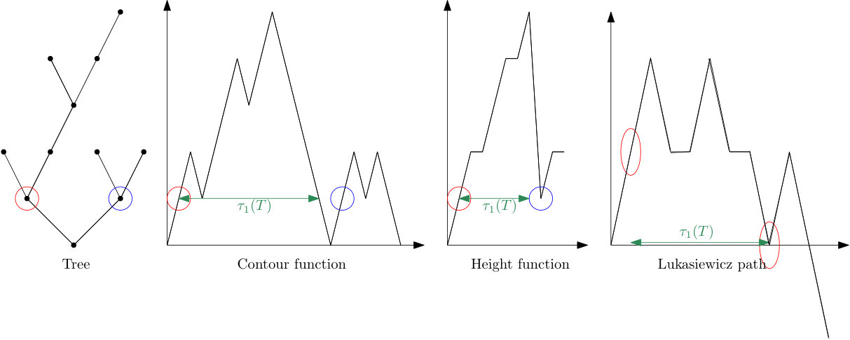 Figure 1
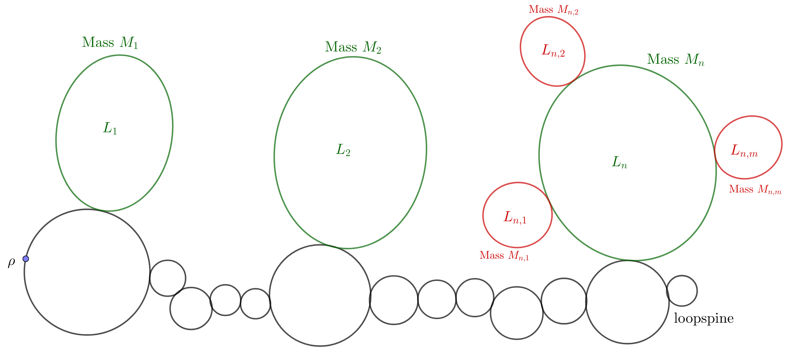 Figure 2
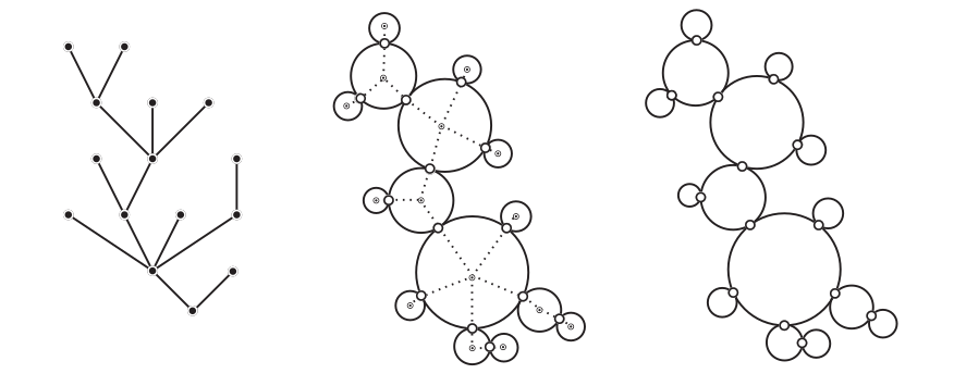 Figure 3
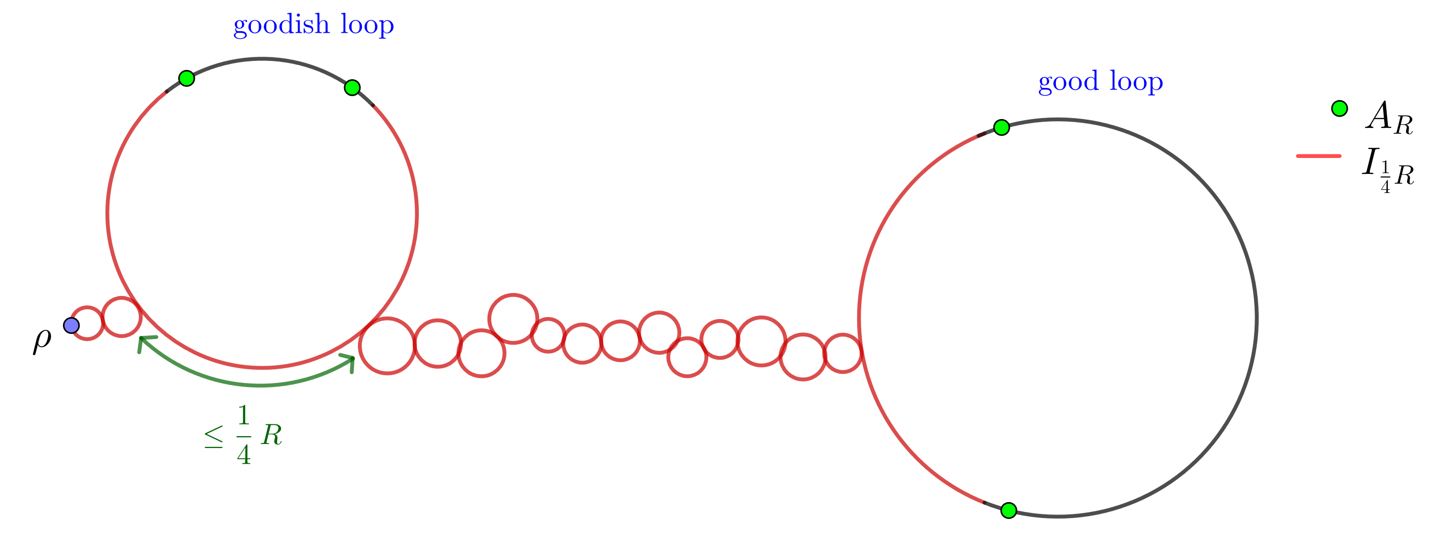 Figure 4
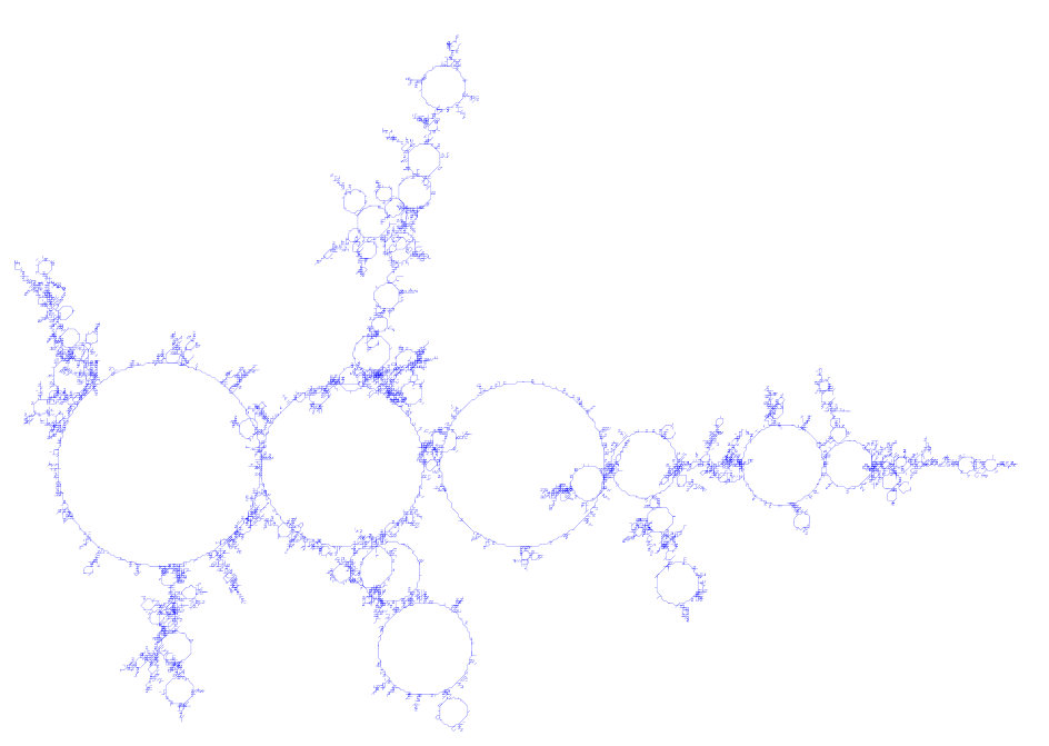 Figure 5
 Figure 6
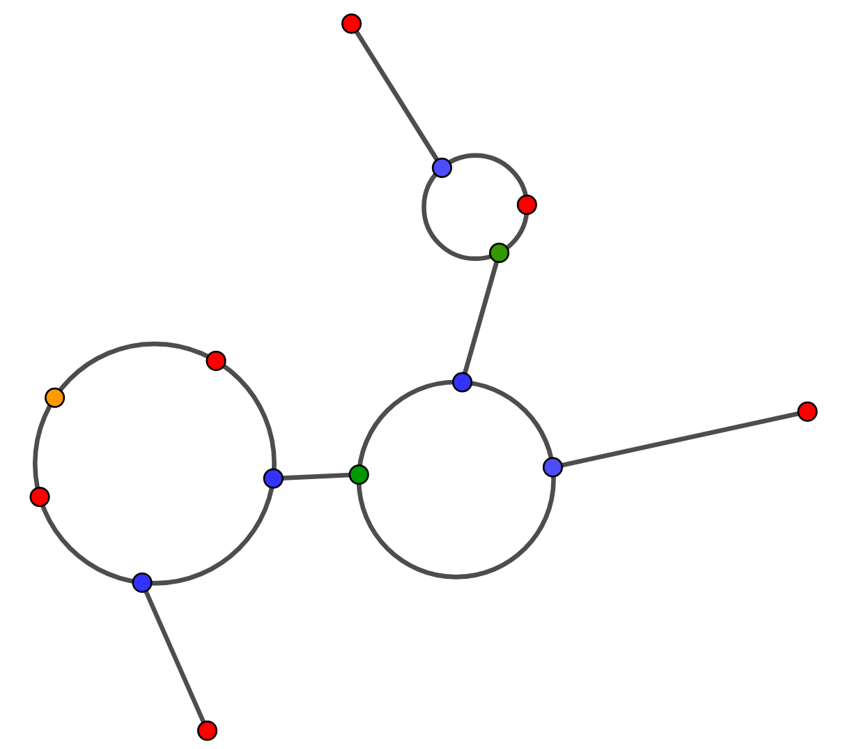 Figure 7
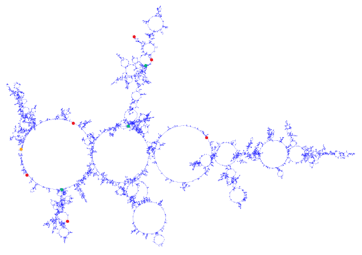 Figure 8
Peer Reviews
No public reviews on file for this paper yet. If you reviewed it on a platform where reviews are public (OpenReview, ICLR, NeurIPS, ICML), you can paste yours below so the community can read it here.
Videos
No videos yet. Explain this paper in a talk, walkthrough, or lecture? Add one.
Brownian motion on stable looptrees
Eleanor Archer Mathematics Institute, University of Warwick, Coventry CV4 7AL, United Kingdom. Email: [email protected].
Abstract
In this article, we introduce Brownian motion on -stable looptrees using resistance techniques, where . We prove an invariance principle characterising it as the scaling limit of random walks on discrete looptrees, and prove precise local and global bounds on its heat kernel. We also conduct a detailed investigation of the volume growth properties of stable looptrees, and show that the random volume and heat kernel fluctuations are locally log-logarithmic, and globally logarithmic around leading terms of and respectively. These volume fluctuations are the same order as for the Brownian continuum random tree, but the upper volume fluctuations (and corresponding lower heat kernel fluctuations) are different to those of stable trees.
AMS 2010 Mathematics Subject Classification: 60K37 (primary), 60F17, 60G57, 60G52, 54E70
Keywords and phrases: random stable looptree, volume fluctuations, heat kernel estimates, stable Lévy process.
1 Introduction
Stable looptrees are a class of random fractal objects indexed by a parameter and can informally be thought of as the dual graphs of stable trees. Motivated by [51], they were originally introduced by Curien and Kortchemski in [26], and along with their discrete counterparts have been shown to be of increasing significance in the study of statistical mechanics models on random planar maps. For example, the same authors showed in [27] that a stable looptree arises as the scaling limit of the boundary of a critical percolation cluster on the UIPT, and Richier showed in [56] that the incipient infinite cluster of the UIHPT has the form of an infinite discrete looptree. Further results along these lines can be found in [27, 25, 58, 9, 28, 48], though this is a very non-exhaustive list. More generally, they also arise as the scaling limits of boundaries of stable maps [57], are closely connected to the shredded stable spheres constructed in [15], and are emerging as an important tool in the programme to reconcile the theories of random planar maps and Liouville quantum gravity [53, 41, 11].
Stable looptrees can be formally defined from stable Lévy excursions but a key result of [26] is an invariance principle characterising them as the scaling limit of discrete looptrees. More precisely, given a discrete tree , the corresponding discrete looptree as defined in [26] is constructed by replacing each vertex with a discrete cycle of length equal to the degree of in , and then gluing these cycles along the tree structure of . Each edge of then naturally corresponds to a vertex of as illustrated in Figure 1. Two vertices in are adjacent if and only they correspond to edges in joining a vertex to two of its consecutive offspring, or else one vertex corresponds to the edge joining to to its parent, and the other vertex corresponds to the edge joining to its first or last child. We give every edge in unit length, and the root of corresponds to the edge of joining its root to its first child. This operation can also be applied in the case where is an infinite tree.
In this article we will be interested in the case where has a critical offspring distribution in the domain of attraction of an -stable law, by which we mean that there exists an increasing sequence such that, if are i.i.d. copies of , then
[TABLE]
as , where is an -stable random variable. In the case , this is equivalent to saying that for some slowly-varying function .
Throughout the article we will make the assumption that , is an offspring distribution in the domain of attraction of an -stable law, and let be the sequence appearing in (1). In [26, Theorem 4.1], it is shown that if is a Galton Watson tree conditioned to have vertices with offspring distribution , then we can define the -stable looptree (denoted ) to be the random compact metric space such that
[TABLE]
in the Gromov-Hausdorff topology as , where denotes the metric space obtained from by multiplying all distances by . A simulation is shown in Figure 2. In the case , the looptrees instead rescale to the Brownian Continuum Random Tree [47, Theorem 2].
The purpose of this article is to introduce and study Brownian motion on stable looptrees, and we start in Section 4 by proving a similar invariance principle that identifies it as the scaling limit of random walks on discrete looptrees, given below. As a consequence, it also follows that the rescaled transition densities and mixing times converge respectively to those of the limiting Brownian motion.
Theorem 1.1**.**
Let be as above, let denote a discrete-time simple random walk on , and let denote Brownian motion on . There exists a probability space on which we can (pointwise) define isometric embeddings of and into a common metric space so that
[TABLE]
almost surely with respect to the Hausdorff metric. In this metric space, we also have that
[TABLE]
as , by which we mean that, almost surely on , the laws of these processes converge weakly on the space ) endowed with the uniform topology.
In fact, we prove a slightly more general version of the theorem that holds for any sequence of discrete trees satisfying the assumptions of [26, Theorem 4.1], but we are mainly interested in applying it in the stable case. The Brownian motion is constructed via the theory of Dirichlet forms and resistance metrics using the now classical theory of [45]. The bulk of this article is then devoted to a detailed study of the resistance volume growth of stable looptrees, from which we obtain heat kernel estimates using results of [18]. The volume growth results also have implications for the Hausdorff and packing measures of stable looptrees with respect to certain gauge functions, for which we prove results analogous to those proved by Duquesne, Le Gall and Wang for stable trees in [33], [34], [36] and [30], and by Croydon for the Brownian continuum random tree (CRT) in [19]. Additionally, the results imply that the packing dimension of is equal to , which is the same as the Hausdorff dimension that was established in [26].
In the past, resistance growth analysis has mainly been useful in studying random walks on trees (for example [19], [22], [23]), since in this case the resistance metric and the geodesic metric are the same. In the case of looptrees the two metrics are different, but we will show that they are equivalent, which allows us to use the two metrics interchangeably when proving the volume bounds.
We will use two main approaches to prove the looptree volume bounds. One approach, used to prove most of the volume lower bounds in this article, builds on ideas of [26] by comparing looptree volume fluctuations with fluctuations in the Lévy excursion that code them. This comparison cannot be used to prove upper bounds however, and a substantial part of this article is devoted to introducing an iterative decomposition of stable looptrees that we use to prove the upper volume bounds. The procedure utilises the Williams’ decomposition of stable trees given in [2] to decompose along a loopspine, breaking it into smaller fragments which are all smaller rescaled looptrees. We then reapply the decomposition to these resulting fragments, and continue to repeat the decomposition on the fragments we obtain each time. This procedure can be realised as a separate branching process, which we will analyse in Sections 5.2 and 5.4 to prove the upper volume bounds.
We now summarise the volume bound results. We will give proper definitions of all the quantities involved in Section 3, but for now we note that denotes the natural analogue of uniform volume measure on stable looptrees. Due to the equivalence of metrics, these results will hold regardless of whether we define the open ball (and its closure ) using the shortest distance metric or the effective resistance metric. As in [26], we denote the -stable looptree by , and its root by . We assume that our looptree is defined on the probability space , and let denote expectation on this space.
We start with the following global (uniform) volume bounds for small balls in , which demonstrate both upper and lower fluctuations of logarithmic order.
Theorem 1.2**.**
-almost surely, there exist constants such that for all :
[TABLE]
[TABLE]
[TABLE]
[TABLE]
We also have the following local (pointwise) results.
Theorem 1.3**.**
-almost surely, for -almost every we have:
[TABLE]
[TABLE]
[TABLE]
[TABLE]
We remark here that the log-logarithmic fluctuations are the same order (up to exponents) as those obtained for a certain class of random recursive fractals in [43], and specifically the same as those obtained for the Brownian CRT in [19, Theorem 1.3]. However, the upper volume fluctuations contrast with those for stable trees which were shown to be logarithmic in [34, Theorem 1.4] when . Intuitively, this is because denser points in stable trees are spread out by larger loops in stable looptrees, creating a more uniform spread of mass. However, the lower fluctuations for stable trees are also log-logarithmic (see [31, Theorem 1.1] and [36, Theorem 1.2]). As in [34] and [31], our results can also be interpreted to give precise bounds on possible gauge functions for exact Hausdorff and packing measures.
The results of Theorem 1.2 show that stable looptrees almost surely satisfy the assumptions of [18, Equation 1.2], and so we can apply the results of that article to deduce that the transition density of the Brownian motion almost surely exists, and study its properties. More precisely, the transition density is a symmetric -measurable function on such that
[TABLE]
for all bounded, -measurable functions on and all . (For reference, a heat kernel is any similar integral kernel so in general is only defined up to a -null set, but in our case, the transition density will be continuous so we will use the two terms interchangeably).
One particular quantity of interest is the spectral dimension of , defined by
[TABLE]
Using [18], we show that almost surely, and also go a step further to obtain the following quenched bounds on the transition density. Here is a deterministic constant, dependent on , that we will write down explicitly in Section 6.
Theorem 1.4**.**
-almost surely, there exist such that
[TABLE]
for all and all . Moreover, it holds -almost surely that
[TABLE]
We also use the local volume bounds of Theorem 1.3 to deduce pointwise heat kernel estimates. Note however that one of the lower bounds in Theorem 1.5 is missing. Heat kernel lower bounds are generally more subtle to obtain than upper bounds, and in particular in this case we would need some additional global volume control to apply the chaining arguments of [18] that are used to prove the corresponding global bound in Theorem 1.4.
Theorem 1.5**.**
-almost surely, for any we have for -almost every that
[TABLE]
We can similarly apply the results of [19] to get off diagonal heat kernel bounds. Once again, and are deterministic constants (dependent on ) and we will give their explicit values in Section 6.
Theorem 1.6**.**
-almost surely, there exist such that for all and all , we have
[TABLE]
Here can denote the distance between and with respect to either the shortest distance metric on , or the effective resistance metric.
A key step in these heat kernel estimates are bounds on the expected exit times from balls, which we will consider in Section 6. Finally, we give an annealed result for the transition density at the root, averaged over the law of . This also implies that the annealed spectral dimension is .
Theorem 1.7**.**
There exists such that
[TABLE]
as .
In light of these results, it also natural to investigate the associated eigenvalue counting function of the Laplacian associated with . More precisely, let be the effective resistance metric on (we will contruct this properly in Section 4), and let be the Dirichlet form associated with the space through the relation
[TABLE]
(this is -almost surely well-defined: see [23, Section 1] for more details on the construction for stable trees; the same principles apply for stable looptrees). We say that is an eigenvalue of with eigenfunction (assumed to be non-trivial) if
[TABLE]
for all . The eigenvalue counting function is then defined as the number of eigenvalues of that are less than or equal to . Due to the representation , any eigenvalue of the operator is also an eigenvalue of . Since is compact and is consequently regular, the converse also holds. Similar arguments to [23] then lead to the following result.
Theorem 1.8**.**
- (i)
For any , as ,
[TABLE] 2. (ii)
-almost surely, as . More over, in -probability, the second order estimate of part (i) holds.
Richier showed in [56] that the incipient infinite cluster (IIC) of the Uniform Infinite Half-Planar Triangulation (UIHPT) has the structure of a discrete looptree, but where each of the loops are filled with independent critically percolated Boltzmann triangulations. The size of the loops of this looptree are given by a distribution in the domain of attraction of a -stable law and the results of our companion paper [6] imply that the boundary of this cluster converges after rescaling to the infinite stable looptree . The question of the scaling limit of the whole cluster is more subtle but is conjectured to be the -stable map [10, Section 5.4], and we hope the methods used in this article will be a good starting point for studying random walks on the IIC. In particular, we anticipate that such a random walk might fall into a framework similar to the discussions of [4], in that the looptree forming the boundary of the IIC may play a role analogous to that of the classical Sierpinski gasket in that article. If this is the case, then understanding random walks on looptrees is a crucial first step to understanding a random walk on the IIC.
Random walks on random infinite discrete looptrees were also studied by Björnberg and Stefánsson in [16] using a generating function approach. As we also prove for in [6], they prove that both the annealed and quenched spectral dimensions of a discrete infinite looptree with critical offspring distribution in the domain of attraction of an -stable law are equal to . Their arguments also exploit the link with resistance growth properties of the space and they show that the volume of a typical ball of radius around the root almost surely undergoes at most logarithmic volume fluctuations around a leading term as . This also gives logarithmic upper and lower bounds on the quenched and annealed transition density at the root. The exponential tail bound in equation (3.18) of their paper suggests however that their volume lower bound fluctuations can also be improved to log-logarithmic order, and we envisage that the approaches of this article can also be applied to their discrete case to give log-logarithmic upper and lower bounds on the volume and transition density fluctuations at typical points. This will be shown in the upcoming article [7].
Finally, in [58], Stefánsson and Stufler show that stable looptrees also arise as scaling limits of outerplanar maps under appropriate conditions on their face weights. Their proof can be adapted to show that this convergence also holds with respect to the resistance metric, with the same scaling exponents, but just with a different scaling constant in front of the metric compared to that of [58, Theorem 3.2]. Moreover, Proposition 4.6 of this paper allows us to extend this to full Gromov-Hausdorff-Prohorov convergence on endowing the outerplanar maps with a uniform measure on their vertices. As a result, we deduce a similar scaling limit for random walks on these outerplanar maps, analogous to Theorem 1.1 (random walks on outerplanar maps will also be treated more explicitly in [7]).
This paper is organised as follows. In Section 2, we introduce some of the technical background used throughout the article. In Section 3, we give formal definitions stable trees and looptrees. In Section 4, we define a resistance metric on stable looptrees, use this to give a construction of the Brownian motion and prove the invariance principle of Theorem 1.1, along with similar convergence results for associated quantities such as transition densities and mixing times. We then prove Theorems 5.18 to 1.3 in Section 5. This is the most substantial section of the paper and is also where we introduce the iterative decomposition procedure mentioned above. Finally, we conclude in Section 6 by proving the heat kernel estimates of Theorems 1.4 to 1.7, and the spectral result of Theorem 1.8.
Throughout this paper, and will denote constants, bounded above and below, that may change on appearance.
Acknowledgements. I would like to thank my supervisor David Croydon for suggesting the problem and for many helpful discussions, as well as the anonymous referees for their detailed and helpful comments on the initial version of this manuscript. I would also like to thank the Great Britain Sasakawa Foundation for supporting a trip to Kyoto during which some of this work was completed, and Kyoto University for their hospitality during this trip.
2 Preliminaries
2.1 Gromov-Hausdorff-Prohorov Topologies
In order to prove convergence results for compact measured metric spaces such as looptrees we will work in the pointed Gromov-Hausdorff-Prohorov topology. Accordingly, let denote the set of quadruples such that is a compact metric space, is a locally finite Borel measure of full support on , and is a distinguished point of , which we call the root.
Suppose and are elements of . Given a metric space , and isometric embeddings of and respectively into , we define d^{GHP}_{M}\big{(}(F,R,\mu,\rho,\varphi),(F^{\prime},R^{\prime},\mu^{\prime},\rho^{\prime},\varphi^{\prime})\big{)} to be equal to
[TABLE]
Here denotes the Hausdorff distance between two sets in , and the Prohorov distance between two measures, as defined in [14, Chapter 1]. The pointed Gromov-Hausdorff-Prohorov distance between and is given by
[TABLE]
where the infimum is taken over all isometric embeddings of and respectively into a common metric space . It is well-known (for example, see [3, Theorem 2.3]) that this defines a metric on the space of equivalence classes of , where we say that two spaces and are equivalent if there is a measure and root preserving isometry between them. The pointed Gromov-Hausdorff distance , which is defined by removing the Prohorov term from (2.1) above, can be helpfully defined in terms of correspondences. A correspondence between and is a subset of such that for every , there exists with , and similarly for every , there exists with . We define the distortion of a correspondence by
[TABLE]
It is then straightforward to show that
[TABLE]
where the infimum is taken over all correspondences between and that contain the point .
In this article, we will prove pointed Gromov-Hausdorff-Prohorov convergence by first proving pointed Gromov-Hausdorff convergence using correspondences, and then show Prohorov convergence of the measures on the appropriate metric space.
2.2 Stochastic Processes Associated with Resistance Metrics
To study Brownian motion and random walks on metric spaces we will be using the theory of resistance forms and resistance metrics, developed by Kigami in [45] and [46].
Let be a discrete graph equipped with non-negative symmetric edge conductances and a measure . Given these conductances, effective resistance on is a function on defined by
[TABLE]
where we take the convention , and is an energy functional given by
[TABLE]
corresponds to the usual physical notion of electrical resistance between and in , when equipped with the given conductances. It can be shown (e.g. see [59]) that is a metric on , and that is a Dirichlet form on .
The notion of a resistance metric can be extended to the continuum as follows.
Definition 2.1**.**
[45, Definition 2.3.2]**. Let be a set. A function is known as a resistance metric on if and only if for every finite subset , there exists a weighted graph with vertex set such that is the effective resistance on , as defined by (11).
A resistance metric on a set can be naturally associated with a stochastic process on via the theory of resistance forms. We do not give details of the theory here, but see [46] for more on resistance forms. In particular, if is a compact metric space, then there is a one-to-one correspondence between resistance metrics and resistance forms on by [46, Corollary 6.4]. Moreover, if is additionally endowed with a finite Borel measure of full support, then by [46, Theorem 9.4], the corresponding resistance form is in fact a regular Dirichlet form on , which in turn is naturally associated with a Hunt process on as a consequence of [39, Theorem 7.2.1].
This correspondence allows us to use results about scaling limits of measured resistance metric spaces to prove results about scaling limits of stochastic processes as detailed in the following result of [20].
Theorem 2.2**.**
[20, Theorem 1.2, compact case]**. Suppose that is a sequence in such that
[TABLE]
with respect to the pointed Gromov-Hausdorff-Prohorov topology for some , and are resistance metrics on the respective spaces.
Let and be the stochastic processes respectively associated with and as outlined above. Then it is possible to isometrically embed and into a common metric space so that
[TABLE]
weakly as probability measures as on (i.e. on the space of càdlàg functions on equipped with the Skorohod -topology).
For more on the Skorohod- topology, see [14, Chapter 3]. The intuition behind the result above is that the convergence of metrics and measures respectively give the appropriate spatial and temporal convergences of the stochastic processes.
It is also the case that we can analyse the associated stochastic processes by analysing the resistance volume growth of the space. This is part of the motivation for proving Theorems 1.2, 1.3 and 5.18, as the heat kernel estimates of Theorems 1.4, 1.5 and 1.7 then follow by an application of results from [18].
2.3 Stable Lévy Excursions
Following the presentations of [29] and [26], we now introduce stable Lévy excursions, which will be used to code stable trees and looptrees in Section 3.
Throughout this article, we take , and will be an -stable spectrally positive Lévy process (i.e. with only positive jumps) as in [12, Section 8], normalised so that
[TABLE]
for all . takes values in the space of càdlàg functions, endowed with the Skorohod- topology, and satisfies the scaling property that for any constant , has the same law as . Moreover, has infinite variation [49, Lemma 2.12], and has Lévy measure
[TABLE]
To define a normalised excursion of , we follow [17] and let denote its running infimum process, and set
[TABLE]
Note that, since has no negative jumps and is of infinite variation, almost surely. Following [17, Proposition 1], we define the normalised excursion of above its infimum at time by
[TABLE]
for every . is almost surely an -stable càdlàg function on with for all , and .
2.3.1 Itô excursion measure
We can alternatively define using the Itô excursion measure. For full details, see [12, Chapter IV], but the measure is defined by applying excursion theory to the process , which is strongly Markov and for which the point [math] is regular for itself. We normalise local time so that denotes the local time of at its infimum, and let denote the excursion intervals of away from zero. For each , the process defined by is an element of the excursion space
[TABLE]
is the lifetime of the excursion . It was shown in [44] that the measure
[TABLE]
is a Poisson point measure of intensity , where is a -finite measure on the set known as the Itô excursion measure.
Moreover, the measure inherits a scaling property from the -stability of . Indeed, for any we define a mapping by , so that (e.g. see [60]). It then follows from the results in [12, Section IV.4] that we can uniquely define a set of conditional measures on such that:
- (i)
For every , . 2. (ii)
For every and every , . 3. (iii)
For every measurable
[TABLE]
is therefore used to denote the law . The probability distribution coincides with the law of as constructed above.
2.3.2 Relation between and
Throughout this paper we will use the following two tools to compare the probability of an event defined in terms of to that of the same event defined in terms of .
Theorem 2.3**.**
[17, Théorème 4]**. Vervaat Transform.
Let be as above, and take Uniform. Then the process defined by
[TABLE]
has the law of a spectrally positive stable Lévy bridge on . 2. 2.
Now let be a spectrally positive stable Lévy bridge on , and let be the (almost surely unique) time at which it attains its minimum. Define an excursion by
[TABLE]
Then has the law of a spectrally positive stable Lévy excursion.
An event defined for the stable bridge on the interval can then be transferred to the unconditioned process using the fact that the law of the bridge is absolutely continuous with respect to the law of the process, with Radon-Nikodym derivative
[TABLE]
for (see [12, Section VIII.3, Equation (8)]).
Here is the transition density of the Lévy process defined above with respect to Lebesgue measure on , i.e. a measurable function on such that
[TABLE]
for all bounded, measurable functions on .
2.4 Two Parameter Poisson-Dirichlet Distribution
We now introduce the two parameter Poisson-Dirichlet distribution, denoted PD(), which arises naturally in the context of decompositions of random trees (amongst other things). It is a law on countable partitions of the interval . We will denote such a partition by . Here we outline the GEM (Griffiths, Engen, McCloskey) construction, which gives a size-biased ordering of the PD() distribution via a residual allocation model. For further background see [55].
Proposition 2.4**.**
[55, Proposition 2]**. For , and , let be a sequence of independent random variables with
[TABLE]
for each . Define a sequence of random variables by
[TABLE]
for all . Then almost surely, and the random vector is distributed as a size-biased ordering of PD().
In Section 5 we will use the following two results.
Lemma 2.5**.**
Let be as above, and let be any sequence of numbers taking values in . Then
[TABLE]
Proof.
This is immediate on noting that . ∎
Lemma 2.6**.**
Let be PD(), where . Then there exists a constant such that for any we have:
[TABLE]
Proof.
The proof is an application of the Paley-Zigmund inequality, which states that for any non-negative random variable with finite variance, and any ,
[TABLE]
By taking , and using the independence of the we have that there exists such that, whenever ,
[TABLE]
The result follows. ∎
3 Background on Stable Trees and Looptrees
3.1 Discrete Trees
Before defining stable trees and looptrees, we briefly recap the Ulam-Harris labelling notation for discrete trees, following the formalism of [54]. Firstly, introduce the set
[TABLE]
By convention, . If and , we let be the concatenation of and .
Definition 3.1**.**
A plane tree is a finite subset of such that
- (i)
, 2. (ii)
If and for some , then , 3. (iii)
For every , there exists a number such that if and only if .
We let denote the set of all plane trees. A plane tree with vertices labelled according to the lexicographical order as can be coded by its height function, contour function, or Lukasiewicz path, defined as follows.
- •
The height function is defined by considering the vertices in lexicographical order, and then setting to be the generation of vertex .
- •
The contour function is defined by considering a particle that starts at the root at time zero, and then continuously traverses the boundary of at speed one, respecting the lexicographical order where possible, until returning to the root. is equal to the height of the particle at time .
- •
The Lukasiewicz path is defined by setting , then by considering the vertices in lexicographical order and setting .
These are illustrated in Figure 3, together with points corresponding to specific vertices in the tree, and the part of each excursion coding the subtree rooted at the red vertex, which we denote by . For further details, see [32, Section 0.1].
These functions all uniquely define the tree . This can be written particularly conveniently in the case of the contour function, since for any , we can write the tree distance as a function on by setting
[TABLE]
We will work mainly with the Lukasiewicz path in this paper. It is not too hard to see that for all , and . Moreover, the height function can be defined as a function of the Lukasiewicz path (see [32, Equation (1)]) by setting
[TABLE]
3.2 Stable trees
We now introduce stable trees. These are closely related to stable looptrees, and were introduced by Le Gall and Le Jan in [50] then further developed by Duquesne and Le Gall in [32, 33]. For we define the stable tree from a spectrally positive -stable Lévy excursion, which plays the role of the Lukasiewicz path introduced above. By analogy with (13), given such an excursion , we define the height function to be the continuous modification of the process satisfying
[TABLE]
where for , and the limit exists in probability (e.g. see [32, Lemma 1.1.3]). We define a distance function on by
[TABLE]
and an equivalence relation on by setting if and only if . is the quotient space , and we let denote the canonical projection from to . If , we let denote the unique geodesic between and in .
This construction also provides a natural way to define a measure on as the image of Lebesgue measure on under the quotient operation.
Stable trees arise naturally as scaling limits of discrete plane trees with appropriate offspring distributions. More specifically, let be a discrete tree conditioned to have vertices and with critical offspring distribution in the domain of attraction of an -stable law, and such that is aperiodic. It is shown in [29, Theorem 3.1] that
[TABLE]
in the Gromov-Hausdorff topology as , where is as defined in (1).
3.3 Random Looptrees
Discrete looptrees are best described by Figure 1 in the introduction. Moreover, as outlined there, stable looptrees can be defined as scaling limits of discrete looptrees: is a Galton Watson tree conditioned to have vertices with critical offspring distribution in the domain of attraction of an -stable law, then
[TABLE]
with respect to the Gromov-Hausdorff topology as [26, Theorem 4.1]. By comparison with (14), can therefore be thought of as the looptree version of the Lévy tree . We now explain how this intuition can be used to code from a stable Lévy excursion, in such a way that can be heuristically obtained from the corresponding stable tree by replacing each branch point by a loop with length proportional to the size of the branch point, and gluing these loops together along the tree structure of .
We first define some notation. As is standard, for every we write if and only if and , and in this case we set
[TABLE]
In what follows we will drop the dependence on and merely write etc.
The following construction was introduced in [26, Section 2.3]. The Lévy excursion itself plays the role of a continuum Lukasiewicz path. It was shown in [52, Proposition 2] that if we define the width of a branch point in , coded by a jump at , by
[TABLE]
then the limit almost surely exists and is equal to . It is therefore natural that a jump of size in should code a “loop” of length in .
Accordingly, for every with , the authors in [26, Section 2.3] equip the segment with the pseudodistance
[TABLE]
and define a distance function on by first setting
[TABLE]
whenever , and
[TABLE]
for arbitrary . They show that as defined above is almost surely a continuous pseudodistance on , and then define an equivalence relation on by setting if , and in [26, Definition 2.3] define the stable looptree as the quotient space
[TABLE]
We let denote the canonical projection under the quotient operation, and let denote the image of Lebesgue measure on under , so that is the natural analogue of uniform measure on .
At various points in this paper, we will refer to the “corresponding” or “underlying” stable tree of , by which we mean the stable tree coded by the same excursion that codes . We let denote a compact stable looptree conditioned on , but at various points we will let denote a generic stable looptree coded by an excursion under the Itô measure but without any conditioning on its total mass. We will also let denote a stable looptree but conditioned so that its underlying tree has height . We will however make any conditioning explicit at the time of writing.
3.3.1 Re-rooting Invariance for Stable Trees and Looptrees
In [33], Duquesne and Le Gall prove that stable Lévy trees are invariant under uniform rerooting. More formally, if is a uniform point in , and we define a new height function from the original height function by
[TABLE]
then . This property is just saying that if we pick a uniform point , and reroot the tree at , then the resulting tree has the same distribution as the original one.
We will prove most of our looptree volume results by considering the volume of a ball at a uniform point in , and then extending to almost all of by Fubini’s theorem. To prove the upper bounds, we will apply some spinal decomposition results for stable trees that we outline in the next section. The uniform rerooting invariance result means that we can equivalently consider our uniform point to correspond to the root of the stable tree.
Note that the problem of uniform rerooting invariance of continuum fragmentation trees was also considered in the paper [42], where the authors additionally show that stable trees are the only fragmentation trees for which this property holds. Duquesne and Le Gall also prove a similar result for rerooting at a deterministic point in the paper [35], and [26, Remark 4.6] directly addresses the question of uniform rerooting invariance for stable looptrees.
4 Resistance and Random Walk Scaling Limit Results
In this section we construct a resistance metric on , define Brownian motion, and prove Theorem 1.1.
4.1 Construction of a Resistance Metric on Stable Looptrees
The metric is similar in spirit to the metric of [26] that we introduced in Section 3.3, but we will sum the effective resistance across loops rather than the shortest-path distance. It turns out that these resistance looptrees are homeomorphic to the original ones, which means that the shortest distance metric can equivalently be used to prove the volume bounds of Theorems 1.2 and 1.3, making the problem more tractable. Additionally this means that part of the invariance principle of Theorem 4.6 arises as a direct consequence of [26, Theorem 4.1].
In the continuum, again let be as in Section 2.3. This time, if has a jump of size at point , equip the segment with the pseudodistance
[TABLE]
The quantity gives the resistance across the loop associated to the branch point at . Note that corresponds to the effective resistance of two parallel edges of resistance and , and by Rayleigh’s Monotonicity Principle it follows that (also see Lemma 4.1).
By analogy with expression (15) in Section 3.3, for with we set
[TABLE]
For arbitrary , we set
[TABLE]
We give a comparison between and in the following lemma.
Lemma 4.1**.**
For any , we have
[TABLE]
Proof.
Note that, trivially, for any :
[TABLE]
Taking we obtain for all , . ∎
It therefore follows from the corresponding result for given in [26, Proposition 2.2] that almost surely, the function is a continuous pseudodistance, and so we can make the following definition. Note in particular that if and only if .
Definition 4.2**.**
Let be an -stable Lévy excursion. The corresponding -stable resistance looptree is defined to be the quotient metric space
[TABLE]
At several points we will write as , to emphasise how it fits into the framework of [20] and various other articles. The next corollary follows directly from Lemma 4.1.
Corollary 4.3**.**
The looptrees and are homeomorphic.
Proposition 4.4**.**
* is a resistance metric in the sense of Definition 2.1.*
To prove Proposition 4.4 we will take a finite set , define a larger graph with , and show that . An illustration is provided in Figure 4. For notational convenience, we will represent by points in that project onto , so suppose , where each , and for . We will also assume that these are the minimal representatives in : that is, if , then with and . We will let denote the projection from into . It then follows from results of [45, Section 2] that we can reduce to an appropriate network on .
Informally, we do this in the natural way: by drawing loops corresponding to points in , and joining these appropriately. In Figure 4, we take to be the set of red points, and form by adding the set of green points that correspond to the most recent common ancestors of pairs of points in . The gold point corresponds to the root of the whole looptree, and the blue points correspond to extra vertices that we denote by expressions of the form below. Formally, we can construct our discrete picture as as follows:
Extend to include all the recent common ancestors of points in . Set
[TABLE] 2. 2.
Draw loops corresponding to points in . Define an equivalence relation on by setting if and only if they have exactly the same set of strict ancestors.
We call each equivalence class a “loop”. Denote the loop corresponding to equivalence class by . If the loop contains only one point in , and if this point is also in , but , then it must be the case that there are no ancestors of in , so we leave it as this one point, and set . If , then we instead draw a loop of length , and mark a point on it as , which we will consider to be the “base” of this loop. If the loop instead contains only one point in but this point is not in then this point must correspond to a recent common ancestor of two points in , and hence is a jump point of the Lévy excursion, say of size . We draw a loop of length and mark as a point on this loop. If contains more than one point, then by definition of it must also contain a point at which has a jump. We denote this point by (note that does not depend on which point we choose to represent the equivalence class). We draw the loop corresponding to by taking all the elements in order so that for all . Note it will then be the case that . Recall also that we are representing points in by their minimal representative in . We then draw the loop corresponding to by adding an edge joining to of length for each , and an edge joining to of length . 3. 3.
Join the loops along the tree structure. We define a partial order on the set of loops by setting if and only if using the ancestral definition of , where we set if contains only one point. For any two loops such that there is no with , join them as follows:
- (i)
If and are both single points, then join these two points with a single edge of length . 2. (ii)
If is a single point but is a loop with at least two points, then join to the point with a single edge of length . 3. (iii)
If contains more than point, but contains a single point, then letting denote the set of ancestors of a point , set , and add a point to the loop at a distance from , where this distance is measured in the direction that respects the lexicographical ordering of points in . Then add an edge joining to of length . 4. (iv)
If both and contain more than one point, then define as above, and join to by an edge of length .
It follows by construction that is a connected graph and . Let denote the effective resistance metric on this graph, which can be calculated using the series and parallel laws. We now prove the following.
Lemma 4.5**.**
[TABLE]
Proof.
The network is in the form of several loops which are joined together by extra edges in such a way as to preserve the tree structure of . For notational simplicity, we now relabel vertices so that , , , and .
Given such that and , let , and let , and similarly . Note that for all . Additionally, write and in lexicographical order. We then have by construction (specifically Step 3 above) and the series law that:
[TABLE]
Then note that by definition (specifically, from Step 3 above), that
[TABLE]
and similarly, by the series law for resistance, we have that
[TABLE]
where the final line follows since for all satisfying .
Similarly, .
It therefore follows from (19), (20) and the series law that
[TABLE]
The cases when and are related differently are dealt with similarly (and more straightforwardly) to show that for all in , thus proving the result. ∎
Since , it then follows from [45, Proposition 2.1.11 and Theorem 2.1.12] that we can reduce to a network with vertex set precisely equal to , and define a metric on to be , the projection of onto , and will be a resistance metric agreeing with on . Proposition 4.4 then follows.
We now prove the following extension of [26, Theorem 4.1].
Proposition 4.6**.**
Let be a sequence of trees with and corresponding Lukasiewicz paths , and let denote the effective resistance metric on obtained via (11) by giving each edge conductance . Additionally let be the uniform measure that gives mass to each vertex of , and let be the root of . Suppose that is a sequence of positive real numbers such that
- (i)
\Big{(}\frac{1}{C_{n}}W^{n}_{\lfloor|\tau_{n}|t\rfloor}(\tau_{n})\Big{)}_{0\leq t\leq 1}\overset{(d)}{\rightarrow}X^{\text{exc}}* as ,* 2. (ii)
* as .*
Then
[TABLE]
as with respect to the Gromov-Hausdorff-Prohorov topology.
Proof.
As a result of Lemma 4.1, Gromov-Hausdorff convergence follows exactly as in the proof of [26, Theorem 4.1] by applying the Skorohod Representation Theorem and then defining a correspondence between and to consist of all pairs of the form or .
To prove that the measures also converge on this space, let , and take the Gromov-Hausdorff embedding endowed with the metric
[TABLE]
We claim that as . For notational convenience we will assume that , and let . Let denote the lexicographical ordering of these vertices. Take a set of vertices in , and let
[TABLE]
Let . We will show that . For any with and for some with . It follows that or , and hence and . It follows that and . Also note that by construction, and so .
Similarly, take a set . We similarly show that . Let , and
[TABLE]
Clearly and so
[TABLE]
If , then there exists with and so . Hence , so and .
It follows that , and hence converges to zero as . ∎
4.2 Random Walk Scaling Limits
In light of Proposition 4.4, we define Brownian motion on to be the diffusion associated with as in Section 2.2. We now show that this is the scaling limit of random walks on discrete looptrees.
Proof of Theorem 1.1.
It follows from Proposition 4.6, separability and the Skorohod Representation Theorem that there exists a probability space on which the convergence of Proposition 4.6 holds almost surely. We will show that on this space, the laws of the given stochastic processes converge weakly, almost surely.
The stochastic process naturally associated with the quadruplet in the sense of Section 2.2 is a continuous time random walk that jumps from its present state to each of its neighbouring vertices at rate . Since every vertex of these discrete looptrees has degree (we consider self-loops as undirected), this amounts to an waiting time at every vertex.
Now define processes and by , and . It follows from Theorem 2.2 that almost surely as , we have the weak convergence
[TABLE]
To deduce the result for in place of , we will show that we can couple the processes and so that they almost surely have the same limit. To do this, note that we can obtain from by sampling a sequence of independent exponential() random variables , letting for all , and setting for all . In particular, for all .
Fix some . Since the limit process is almost surely continuous, the convergence of (21) actually holds with respect to the uniform topology. By again appealing to the Skorohod representation theorem along with a functional law of large numbers, we can therefore restrict to a probability space where \big{(}(\tilde{Y}_{t})_{t\in[0,T]},\big{(}(na_{n})^{-1}S^{(n)}_{\lfloor 4C_{\alpha}n^{1+\frac{1}{\alpha}}t\rfloor}\big{)}_{t\in[0.T]}\big{)}\rightarrow((B_{t})_{t\in[0,T]},t) jointly almost surely.
By composing these continuous limits, we therefore deduce that
[TABLE]
uniformly almost surely. This proves that the distributional result holds for arbitrary , and we extend to all time by applying [14, Lemma 16.3]. ∎
Remark 4.7**.**
It is also possible to deduce an annealed convergence result by embedding into the universal Urysohn space. We will not pursue this further here, but refer to [6, Section 2.2] for full details.
Remark 4.8**.**
It also follows from [21, Theorem 1 and Proposition 14] that the transition densities of the discrete time random walks on any compact time interval will converge to those of under the same rescaling when we isometrically embed in the space as described above. This can be metrized using the spectral Gromov-Hausdorff distance, introduced in [24, Section 2]. It also follows by an application of [24, Theorem 1.4] that for any , the rescaled -mixing times for will converge to those of . We expect that we can prove similar convergence results for blanket times using ideas of [5], and that the sequence of cover times will be Type 2 in the sense of [1, Definition 1.1].
5 Volume Bounds for Compact Stable Looptrees
In this section we prove Theorems 1.2 and 1.3. Recall that denotes the law of , and we let be . For ease of intuition, we define the open ball using the metric rather than .
5.1 Infimal Lower Bounds
We prove the lower volume bounds of Theorems 1.2 and 1.3 via the following proposition.
Proposition 5.1**.**
There exist constants such that for all and all ,
[TABLE]
The proof of Proposition 5.1 uses ideas from the proof of the upper bound on the Hausdorff dimension of that was given in [26, Section 3.3.1]. It relies on the fact that for any with ,
[TABLE]
This result appears as [26, Lemma 2.1]. Consequently, we can lower bound the volume of small balls in by upper bounding the oscillations of . We use the notation to denote the diameter of the set defined from using the distance function of (16), but with in place of .
We first give a technical lemma which appeared previously in [26, Section 3.3.1] and uses an argument from [12]. The final claim follows by bounded convergence.
First recall that for a function and , we define
[TABLE]
Lemma 5.2**.**
Let be an exponential random variable with parameter , and let be a spectrally positive -stable Lévy process conditioned to have no jumps of size greater than on . Let . Then there exists such that . Moreover, as .
Remark 5.3**.**
The same results holds if is set to be deterministically equal to rather than an exponential random variable. The proof is almost identical to the one above, with one minor modification.
Proof of Proposition 5.1.
First, note the inclusion
[TABLE]
By applying the Vervaat transform, the absolute continuity relation (12) and scaling invariance, we get that
[TABLE]
To bound the latter quantity, let be the cardinality of the set , where now denotes the jump size of rather than , and let be its members in increasing order of size. Additionally let and , and , so that . We then have:
[TABLE]
where is as in Remark 5.3. Note that and are not independent, but we certainly have for all , and hence by Lemma 5.2 and Remark 5.3 we can choose small enough that . The result follows from noting that
[TABLE]
∎
By taking a union bound, the same argument can be used to give a bound on the global infimum.
Proposition 5.4**.**
There exist constants such that for all and all ,
[TABLE]
Proof.
By the same reasoning as in the proof of Proposition 5.1, we have:
[TABLE]
and hence
[TABLE]
where the final line follows by Proposition 5.1. ∎
Proof of infimal lower bounds in Theorems 1.2 and 1.3.
Take as in Proposition 5.1, and . Set
[TABLE]
Taking in Proposition 5.1 we see that , and since we have by Borel-Cantelli that . Hence there almost surely exists such that occurs for all . On this event, for all sufficiently small , or equivalently,
[TABLE]
To deduce the result for -almost every we apply Fubini’s theorem. Letting
[TABLE]
we have from above that
[TABLE]
By Fubini’s theorem, this implies that almost surely, for Lebesgue almost every , and consequently for -almost every . This proves (6).
The proof of the global bound (2) is similar. Take as in Proposition 5.1, choose some , and set . Then, setting we have by Proposition 5.4 that:
[TABLE]
Consequently, letting
[TABLE]
we have by Borel-Cantelli that . Hence, there almost surely exists a such that for any we have (2), or more precisely that:
[TABLE]
∎
5.2 Supremal Upper Bounds
In this section we prove (3) and (7) using the following Williams’ Decomposition. By appealing to uniform re-rooting invariance, we will treat as the root of the looptree throughout.
5.2.1 Williams’ Decomposition
The Williams’ Decomposition of [2] gives a decomposition of a stable tree along its spine of maximal height. In the Brownian case , this corresponds to Williams’ decomposition of Brownian motion. Letting , we see from [37, Equation (23)] (and references therein) that there is almost surely a unique such that . We define the Williams’ spine (or W-spine) of to be the segment , and take the Williams’ loopspine (or W-loopspine) in the corresponding looptree to be the closure of the set of loops coded by points in . A main result of [2] is a theorem which firstly gives the distribution of the loop lengths along the W-loopspine, and additionally the distribution of the fragments obtained by decomposing along it.
Given the spine from to , and conditional on , the loops along the W-loopspine can be represented by a Poisson point measure on with a certain intensity. A point corresponds to a loop of length in the W-loopspine, occurring on the W-spine at distance from the root in the corresponding tree , and such that a proportion of the loop is on the “left” of the W-loopspine, and a proportion is on the “right”. In [2], this is written in terms of the exploration process on , but we interpret their result below in the context of looptrees.
We note that when stating this result, we are not conditioning on the total mass of : only the maximal height. The mass will depend on its height via the joint laws for these under the Itô excursion measure.
Theorem 5.5**.**
(Follows directly from [2, Lemma 3.1 and Theorem 3.3]).
- (i)
Conditionally on , the set of loops in the W-loopspine forms a Poisson point process on the W-spine in the corresponding tree with intensity
[TABLE]
where is the underlying Lévy measure, with in the stable case. We will denote the atom by . 2. (ii)
Let be an atom of the Poisson process described above. The set of sublooptrees grafted to the W-loopspine at a point in the corresponding loop can be described by a random measure , where is a Lévy excursion that codes a looptree in the usual way, and represents the distance going clockwise around the loop from the point at which this sublooptree is grafted to the loop, to the point in the loop that is closest to . This measure has intensity
[TABLE]
In particular, the sublooptrees are just rescaled copies of our usual normalised compact stable looptrees, and each of these is grafted to the loop on the W-loopspine at a uniform point around the loop lengths.
Remark 5.6**.**
Point is a slight extension of the results of [2], where the authors write that the intensity of subtrees incident to the W-spine at a node of “degree” has intensity . However, it follows from [33, Equation (11)] and the remarks below it that the corresponding sublooptrees are actually distributed uniformly around the corresponding loop.
5.2.2 Encoding the Looptree Structure in a Branching Process
The Williams’ decomposition suggests a natural way to encode the fractal structure of in a branching process or cascade. Specifically, we let denote the root vertex of our cascade. This represents the whole looptree (in particular, should not be confused with , which is the root of ). By performing the Williams’ decomposition on and removing the W-loopspine, the fragments obtained are countably many smaller copies of , which we view as the children of in our branching process, and index by . Moreover, to each edge joining to one of its offspring , we associate a random variable which gives the mass of the sublooptree corresponding to index . The root of a sublooptree is the point at which it is grafted to the W-loopspine of its parent.
We can then perform further Williams’ decompositions of these sublooptrees. More precisely, if is a child of , we can decompose along its W-loopspine from its root to its point of maximal tree height to obtain a countable collection of offspring of that correspond to the fragments obtained on removing this W-loopspine, and label the offspring as . By repeating this procedure again and again on the resulting subsublooptrees, we can keep iterating to obtain an infinite branching process.
Remark 5.7**.**
It may seem more straightforward to use a spinal decomposition to a uniform point (as in [42]) as the basis of this iteration, rather than the Williams’ decomposition. However, this leads to technical difficulties in the case when is chosen so that is a point too close to , and it is convenient to avoid this by instead decomposing along the maximal spine in the underlying tree.
We index this process using the Ulam-Harris labelling convention defined in Section 3.1. Using the notation of [54], an element of our branching process will be denoted by , and corresponds to a smaller sublooptree . Its offspring will all be of the form , with corresponding roots , where here abbreviates the concatenation , and each will correspond to one of the further sublooptrees obtained on performing a Williams’ decomposition of .
Moreover, to each edge joining to its child we associate a random variable . These give the ratios of the masses of each of the sublooptrees that correspond to the offspring of , so that for all . Given a particular element of the branching process, the overall mass of the corresponding sublooptree is then given by , where here we let denote the root .
5.2.3 Main Argument for Supremal Upper Bound
The simplest way to upper bound the volume is to sum the masses of all the sublooptrees that are incident to the W-loopspine at a point within distance of , giving
[TABLE]
We would like to use this to bound . However, this approach is not very sharp since the probability that there is such an incident sublooptree of mass greater than is of order , and when this happens the bound on the right hand side of (24) is immediately too large. However, if this event occurs, it is actually likely that this sublooptree is not completely contained in , and so we are not really capturing the right asymptotics for the behaviour of by applying (24).
To refine the argument we instead repeat the same procedure around the W-loopspine of the larger sublooptree. If there are no larger (sub)sublooptrees incident to the (sub)W-loopspine close to the (sub)root, then we conclude by summing the smaller terms; otherwise, we can keep repeating the same procedure and iterating further until eventually we reach a stage where there are no more “large” sublooptrees to consider.
This iterative process corresponds to selecting a finite subtree of in such a way that the elements of correspond to the large sublooptrees around which we perform further iterations. The offspring distribution of will be sufficiently subcritical that the process will die out fairly quickly. Conditioning on the extinction time and then on the total progeny of , we bound the volume of the ball by the sum of the masses of all the small sublooptrees that are grafted to the W-loopspine of each of the large sublooptrees.
Below, we describe how we select generation by generation as a subtree of . Throughout, we take:
[TABLE]
Note that . Also fix some \kappa\in\big{(}0,\big{(}\frac{1}{3e^{2}}\Gamma(1-\frac{1}{\alpha})\big{)}^{\alpha}\big{)}. We need to be sufficiently small to ensure that is sufficiently subcritical, but we will not be taking any kind of limit as .
**Iterative Algorithm
**
Start by taking to be the root of . Recall this represents the whole looptree .
Perform a Williams’ decomposition of along its W-loopspine.
Consider the resulting fragments. To choose the offspring of , select the fragments that have mass at least , and such that the subroots of the corresponding looptrees are within distance of the root of .
Repeat this process to construct one generation at a time. Given an element , there is a corresponding sublooptree in with root and . Consider the fragments obtained in a Williams’ decomposition of , and select those that correspond to further sublooptrees that are within distance of , and also such that they have mass at least (i.e. with ), to be the offspring of .
For each , set
S_{u}=\sum_{i=1}^{\infty}M_{ui}\mathbbm{1}\Big{\{}\rho_{ui}\in B(\rho_{u},r)\Big{\}}\mathbbm{1}\Big{\{}M_{ui}<\kappa^{-1}r^{\alpha}\lambda^{1-\beta_{1}-\beta_{2}}\Big{\}}.
As explained above, in the event that is finite we then have that:
[TABLE]
Since the Williams’ decomposition involves conditioning on the height of the corresponding stable tree rather than its mass, we will prove this theorem by rescaling each sublooptree corresponding to an element of to have underlying tree height , and then using Theorem 5.5 to analyse the fragments. Most of the effort in proving the supremal upper bounds is devoted to proving the following proposition.
Proposition 5.8**.**
There exist constants such that for all and all ,
[TABLE]
The volume results (3) and (7) follow from Proposition 5.8 by Borel-Cantelli, similarly to those in the previous section. We sketch this below, and prove Proposition 5.8 afterwards.
Proof of supremal upper bounds of Theorems 1.2 and 1.3, assuming Proposition 5.8.
Take as in Proposition 5.8, and choose some . Taking in Proposition 5.8 and applying Borel-Cantelli we deduce that , where
[TABLE]
Similarly to the proof of the infimal bounds, it follows that
[TABLE]
almost surely, and we extend to -almost every using Fubini’s theorem as before. This proves (7).
To prove the global bound (3), we have to do a bit more work. First take some , and define to be the set of sets
[TABLE]
where takes the same value as it did in Proposition 5.4. It then follows from Proposition 5.4 that
[TABLE]
for all sufficiently small . Moreover, assuming that is indeed an -covering of , and letting
[TABLE]
be the -fattening of for any set , say with
[TABLE]
we have that . It hence follows that
[TABLE]
and consequently,
[TABLE]
It follows from rerooting invariance at deterministic points that for any ,
[TABLE]
and hence by applying a union bound and Proposition 5.8, we see that
[TABLE]
In particular, taking , where is as it was in Proposition 5.8, we obtain
[TABLE]
By combining equations (25), (26) and (27), we therefore see that
[TABLE]
Hence, letting , we have as before that . This implies (3), since similarly to before, we deduce that there exists such that for all ,
[TABLE]
∎
For a given looptree and a given , we let denote the set of points in the W-loopspine that also fall within distance of the root. Formally,
[TABLE]
where is the Lévy excursion coding . can be endowed with a natural notion of length, denoted , which can be thought of as the sum of the lengths of loop fragments contained in . Formally, this can be defined as the Lebesgue measure of the closure of the set .
To bound the progeny of , we can then use the Williams’ decomposition to view the sublooptrees grafted to the W-loopspine as a Poisson process on . In particular, the number of sublooptrees with mass greater than will be stochastically dominated by a Poisson with parameter , where denotes the Itô excursion measure and denotes the length of an excursion under this measure. will be roughly of order , but the purpose of the next lemma is to control this more precisely.
Lemma 5.9**.**
Let be a compact stable looptree conditioned so that its underlying tree has height , but with no conditioning on its mass. Take , and let and be as above. Then
[TABLE]
Proof.
It is possible that may be of order greater than if, for example, many of the loops close to the root have spinal branch points distributed such that they split the loop into two very unequal segments. We show that this occurs only with very low probability.
First note that, by Theorem 5.5(i), the loops that fall on the first half of the W-spine stochastically dominate a Poisson point measure with intensity
[TABLE]
Elements of the set correspond to distances along the spine in the underlying tree, but we will consider them as time indices throughout the remainder of this proof. We will model the loop lengths using a subordinator, where a jump of the subordinator of size at time corresponds to a loop of length which in turn corresponds to a node at a distance along the W-spine in the associated stable tree.
To prove the bound, we first condition on existence of a loop in the W-loopspine with length greater than and with . We say that such a loop is “good”. We also say that a loop is “goodish” if it just has length at least , with no restriction on . We then select the closest good loop to . Given such a loop, the number of goodish loops between and the first good loop is stochastically dominated by a Geometric() random variable. Letting this number be , can then be upper bounded by the random variable
[TABLE]
where denotes the sum of the lengths of all the smaller loops on the W-loopspine that are between the and goodish loops, and the term comes from selecting a segment of length at most in each direction from the “base point” around each of the goodish loops. Each can be independently approximated by an -stable subordinator run up until an exponential time and conditioned not to have any jumps greater than .
First let the number of good loops on the first half of the W-spine be equal to . From (28), it follows that stochastically dominates a Poisson random variable with parameter
[TABLE]
where is just a constant. Hence,
[TABLE]
We henceforth condition on . Next, note that for any loop of length at least , the probability that it is good is at least (independently of the other loops), and so if we examine all such loops of the W-loopspine in order from , as described in the previous paragraph, we have that is stochastically dominated by a Geo() random variable. Hence, for any , we have by a Chernoff bound that
[TABLE]
To bound , we again use (28). Conditionally on , (28) implies that the times between each successive pair of goodish loops in the W-loopspine will each be independently stochastically dominated by an exp() random variable, which we denote by . Hence, the sum of the smaller jumps between each pair can be stochastically dominated by , where Sub is a subordinator with Lévy measure
[TABLE]
Also let be an exp() random variable (recall that ). It further follows by rescaling that
[TABLE]
where are independent copies of Sub, and are independent copies of a subordinator similar to Sub but with Lévy measure
[TABLE]
It then follows by Lemma 5.2 that there exists such that . For such , we hence have
[TABLE]
To conclude, we combine the results of (29), (30) and (31) by writing
[TABLE]
∎
The second technical lemma will allow us to bound the total progeny of by comparing it to a subcritical Galton-Watson tree with Poisson offspring distribution.
Lemma 5.10**.**
Let be a compact stable tree, and be its corresponding compact stable looptree, both coded by the same excursion under the Itô measure but conditioned to have lifetime at least . Let be the root of , and perform a Williams’ decomposition of along its W-loopspine. Let denote the number of resulting sublooptrees obtained that are of mass at least and are also grafted to the W-loopspine within distance of the root of . Then
[TABLE]
where K_{\alpha}=3\big{(}\Gamma\big{(}1-\frac{1}{\alpha}\big{)}\big{)}^{-1}\kappa^{\frac{1}{\alpha}}. The constants and also depend on , but is fixed and the precise dependence will not be important, so we suppress this notationally.
Proof.
Let be the height of , and let be the rescaled excursion given by
[TABLE]
The excursion codes a tree conditioned to have height (this can be seen from combining [40, Lemma 5.8, Part 3] with [37, Equation (26)], for example). Moreover, in the corresponding looptree, now denotes the number of sublooptrees of mass at least that are grafted to the W-loopspine within distance of .
We wish to bound so that we can apply Lemma 5.9. To do this, note by monotonicity and scaling invariance that
[TABLE]
where the final line holds by [37, Theorem 1.8]. Then, conditioning on (i.e. ), we have by Lemma 5.9 that
[TABLE]
By Theorem 5.5(ii), the sublooptrees grafted to the W-loopspine at points in form a Poisson process of sublooptrees coded by the Itô excursion measure, but thinned so that none have height large enough to violate the condition that the end of the W-spine corresponds to the point of maximal height in the tree. We can therefore stochastically dominate this by the unthinned (classical) version of the Itô excursion measure of Section 2.3.1. Since , where (e.g. see [40, Proposition 5.6]), it follows that conditionally on , is stochastically dominated by a Poisson random variable with parameter:
[TABLE]
To conclude, we write:
[TABLE]
∎
Armed with these lemmas, there are now two key steps to the main argument. One of these is to bound the number of times we need to reiterate around larger sublooptrees as described by the algorithm, and the other is to bound the contributions of smaller terms from each of these iterations.
As is usual, we will let denote the total progeny of the tree . The first main result is the following.
Proposition 5.11**.**
There exist constants such that
[TABLE]
Proof.
The main ingredient in this proof is the main theorem of Dwass from [38], that for a Galton-Watson tree with total progeny Prog and offspring distribution , it holds that
[TABLE]
where the are i.i.d. copies of . In particular, if for some we see by writing the sum explicitly and applying Stirling’s formula that
[TABLE]
This isn’t a priori applicable since in our case is not quite a Galton-Watson tree. However, it follows from Lemma 5.9 that for any , we have
[TABLE]
where is a Galton-Watson tree with Poisson() offspring distribution. Accordingly, setting (which is less than by our choice of ) and we see that
[TABLE]
so combining with the above we deduce that
[TABLE]
as claimed. ∎
Proposition 5.12**.**
Conditional on , we have that
[TABLE]
Proof.
Take , and let be the corresponding (sub)looptree that forms part of . By the same arguments used in Proposition 5.11, we can use Lemma 5.9 to show that, letting , we have
[TABLE]
We now condition on . Again dominating the thinned Itô excursion measure by the classical Itô excursion measure as we did in the proof of Proposition 5.12, we have that is stochastically dominated by a subordinator with Lévy measure , run up until the time . Note that the Lévy measure coincides with that of an -stable subordinator, conditioned to have no jumps greater than .
Hence, letting Subord be an -stable subordinator, and conditioning on , we have by scaling invariance that:
[TABLE]
By the arguments of Lemma 5.2, it follows that there exists such that when conditioned to have no jumps greater than , so, as before, the latter probability can be bounded by .
Combining these, we see that
[TABLE]
The result follows on taking a union bound. ∎
We are now able to prove Proposition 5.8.
Proof of Proposition 5.8.
Note that, on the events and , we have that
[TABLE]
Hence, by combining the results of Propositions 5.11 and 5.12, we see that
[TABLE]
∎
5.3 Supremal Lower Bounds
In this section, we prove (4) and (8). We start by proving a probabilistic bound. The proof relies on using the relation (22) to compare volume fluctuations with stable Lévy oscillations.
Proposition 5.13**.**
There exist constants such that for all and all ,
[TABLE]
Proof.
As explained in Section 5.1, we know that
[TABLE]
It follows from the scaling relation that as whenever . Consequently, by applying the Vervaat transform and the absolute continuity relation, we have for all sufficiently small values of that
[TABLE]
where denotes the exit time of from the interval , conditioned on .
It follows from the discussion below Theorem 2 of [13] that , for some deterministic constants . The proposition follows. ∎
We cannot directly use Proposition 5.13 to prove the lower supremal bounds since we do not have the necessary independence to immediately apply the second Borel-Cantelli lemma. However, we can achieve this by performing a spinal decomposition, and considering volumes in different fragments, which are independent of each other. To do this, we will use a spinal decomposition to a uniform point, detailed below. The advantage of this over the Williams’ decomposition in this case is that it allows us to control the masses of individual fragments more explicitly.
5.3.1 Spinal Decomposition from the Root to a Uniform Point
In [42], it was shown that if we define the spine of a stable Lévy tree to be the unique path from the root to a uniform point, then can be broken along this spine and that the resulting fragments form a collection of smaller Lévy trees. This gives a similar decomposition result for looptrees.
We define the decomposition formally as follows. Let , so that is a uniformly chosen vertex in , and let be its root. We say that the loopspine from to , denoted , is the closure of the set of loops corresponding to ancestors of . To form the fine spinal decomposition, first let be the connected components of , and then for each let be the closure of in . Then almost surely, each can be written in the form for some . Note that by uniform rerooting invariance, we can also replace the root with an independent uniform point in .
If the fragment has mass , define a metric and a measure on by
[TABLE]
Additionally let be a vertex in chosen uniformly according to . We then have the following result, which is a consequence of [42, Corollary 10], which gives the corresponding result for Lévy trees.
Theorem 5.14**.**
* is a collection of independent copies of . Moreover, the entire family is independent of , which has a Poisson-Dirichlet distribution.*
5.3.2 Main Argument for Supremal Lower Bound
Using Theorem 5.14, we can construct an argument as follows. First take some with . Given , and a decreasing function of such that as , define the interval . It is easy to verify that for all sufficiently small , the intervals and are disjoint.
Our strategy is as follows. We use the spinal decomposition of Section 5.3.1, between and an independent uniform point . Recall the GEM distribution introduced there, that gives a size biased representation of the Poisson-Dirichlet distribution. Letting denote the segment of loopspine that intersects (analagously to defined in Section 5.2.3), there is probability of order at least that there is a such that the sublooptree with Poisson-Dirichlet mass given by the GEM random variable is grafted to the loopspine at a point in . Say this sublooptree is , with root being the point at which it is grafted to the loopspine. The mass of the ball is then lower bounded by the mass of . We can then rescale the looptree , and the corresponding unit ball, to compute that this mass is at least with at least polynomial probability. We repeat this argument along the sequence . Since the corresponding intervals are disjoint (provided we start at a sufficiently large value of ), and the rescaled looptrees from the spinal decomposition of Section 5.3.1 are independent, we obtain the necessary independence to apply the second Borel-Cantelli Lemma.
Proof of supremal lower bound in Theorem 1.3.
Let be the length of the loopspine, and let be the total number of sublooptrees in the spinal decomposition that are incident to the loopspine at a point in and have mass corresponding to a GEM index in . Then, conditional on , stochastically dominates a random variable that is Binomial(). Hence, the probability that this number is non-zero is at least of order .
Conditional on , let be an index in with corresponding sublooptree that is incident to the loopspine at a point in . Note that stochastically dominates the Poisson-Dirichlet GEM weight , where , and hence we have by Lemma 2.6 that there exists such that
[TABLE]
Conditional on there being such a sublooptree , say of mass , we know that
[TABLE]
by Proposition 5.13 (note in particular that as so it is fine to apply the result here).
Hence, letting be the event that there exists a sublooptree incident to the loopspine at a point in with GEM index , and such that the ball of radius in this sublooptree has mass at least , we deduce that .
Now, letting , we have that there exists a finite such that the intervals and are disjoint whenever , and hence since each sublooptree is distributed uniformly around the perimeter of the loopspine independently of the others, then the events that there exist sublooptrees with GEM index in (respectively ) within distance (respectively ) from the root are independent events. Moreover, if the sublooptrees described in the events and exist, then they are independent once rescaled by Proposition 5.14. Thus the only dependence between the events and is in whether these sublooptrees have masses greater than (respectively ), but here the only dependence is that all the Poisson-Dirichlet masses must sum to , and hence in actual fact by an application of Lemma 2.5.
Hence,
[TABLE]
so setting we see that . Since is almost surely finite, we can integrate over possible values of to deduce that .
The result at (8) follows by applying Fubini’s theorem similarly to the previous extremal volume bounds. ∎
The proof of the global bound given in (4) uses a similar decomposition approach, but this time we perform two subsequent spinal decompositions. This is illustrated in Figure 5. Firstly, let denote the GEM masses obtained on performing a first spinal decomposition of . Then, for each of the resulting fragments , rescale to obtain a sequence of independent stable looptrees , each with mass . For each , we perform a further spinal decomposition of and denote the resulting GEM masses by , and corresponding looptrees by , and by after rescaling again to have mass . We take , and , where is a specific constant to be specified later. We also define the events:
[TABLE]
Also set , and define the event
[TABLE]
The key point is to observe that , so it is sufficient to show that . The next lemma gives a means to overcome the dependencies between the GEM masses and apply the second Borel-Cantelli Lemma. It should be intuitively clear, but we give a proof for completeness.
Lemma 5.15**.**
Let be as above. Then
- (i)
, 2. (ii)
.
Proof.
First, note that since the individual looptrees in the spinal decomposition are independent of each other and of their original masses once rescaled, we can make the following observations:
- •
is independent of for all and all ,
- •
is independent of for all and all ,
- •
Conditional on , is independent of for all .
Figure 5 may be helpful to keep track of the dependencies. In fact, the only dependence between these events is of the form described by Lemma 2.5.
We start by proving . First note that by the first independence stated above, we have that
[TABLE]
We focus on the first term in the final line above. By the second independence stated above, we have that
[TABLE]
where for :
[TABLE]
Since is independent of , we can apply Lemma 2.5 to deduce that for all . Substituting this into the final line, we obtain
[TABLE]
We can use the same kind of expansion and apply Lemma 2.5 to show that
[TABLE]
Point then follows from the final line of (34). The proof of the point is almost identical, so we omit it. ∎
Armed with the lemma, we prove the global infimum upper bound as follows.
Proof of supremal lower bound in Theorem 1.2.
Recall from Theorem 5.14 that the rescaled looptree is independent of . It follows that the event is independent of , and hence
[TABLE]
We bound each of these terms separately. Firstly, by Lemma 2.6, we have that there exists such that
[TABLE]
for all . Recalling that , we see that
[TABLE]
To bound the second term in (35), we apply point of Lemma 2.5, which implies that
[TABLE]
Recalling that , we again apply (36) to deduce that
[TABLE]
whenever . To conclude, note that conditional on , we have that and hence we can apply Proposition 5.13 to deduce that
[TABLE]
Here we are specifically taking to be the constant in the exponent of Proposition 5.13. Combining, we see that
[TABLE]
Hence, by choosing , we see that as , and in particular that we can lower bound it by a non-negative constant uniformly in . Combining this with (35) and (36), we see that there exists a constant such that for all . It then follows from Lemma 5.15 and Borel-Cantelli that .
The conclusion follows since on the event , we can rescale the ball back to its original size in the original looptree to obtain a ball of radius with volume at least . Moreover, on the event we also have that , so this volume is actually lower bounded by . ∎
5.4 Infimal Upper Bounds
We now prove (5) and (9). The method we use to prove upper bounds on infimal extrema is a simpler version of that used in Section 5.2 based on the Williams’ decomposition. We can again control the masses of fragments in the decomposition by comparison with an -stable subordinator. In this case however, we do not need to worry about reiterating around larger fragments since the presence of such fragments is a rare event and thus should not affect the infimal behaviour of the subordinator.
Let be the height of the spine in the corresponding tree . As in Section 5.2, we start by rescaling by to form the looptree , which now has mass and has a corresponding underlying stable tree that has height . Note that
[TABLE]
where again . As explained in the Lemma 5.10, and using the notation we introduced there, it follows from properties of the Itô excursion measure that is stochastically dominated by , where is an -stable subordinator, and denotes the length of W-loopspine that intersects . A jump of of size at a time corresponds to a sublooptree coded by an Itô excursion of lifetime equal to , and grafted to the W-loopspine at a point that informally is at a clockwise distance “through” . Moreover, since we have rescaled the looptree to have tree height , there is no constraint on its total mass, and therefore no dependence between different jumps of .
For technical reasons we will in fact model this by two independent -stable subordinators, and , corresponding to the left and right sides of the W-loopspine respectively. We set .
The comparison relies on the following result, which gives the limiting behaviour of the infimum of an -stable Lévy subordinator.
Theorem 5.16**.**
[12, Section III.4, Theorem 11]**. Let be an -stable Lévy subordinator. Then, almost surely,
[TABLE]
To deduce a similar result for in place of , note that the only difference between the two subordinators is the constant in the Lévy measure. Hence we have the same result for , but just with a different constant on the right hand side. We will denote this constant by .
Proof of local infimal upper bound in Theorem 1.3.
Set for . By Theorem 5.16, there almost surely exists a sequence with such that
[TABLE]
for all . Since whenever , we can extract a subsequence if necessary so that
[TABLE]
and also for all . Set .
Note that since the process depends only on the total length of the W-loopspine, and not on its microscopic structure, it follows from Lemma 5.9 that there exists a constant such that
[TABLE]
for all . More specifically, we let be the event described by taking in the proof of Lemma 5.9 that ensures that , consisting of the three subevents:
There exists a good loop in the W-loopspine with total length in .
There are no goodish loops in the W-loopspine occurring between the root and the first good one.
The sum of the lengths of the smaller loops up until the first good loop is upper bounded by .
The proof of Lemma 5.9 ensures that for all , but to apply the second Borel-Cantelli Lemma we need to lower bound instead. To do this, note that conditional on :
- •
The probability of the event described in is unaffected by the events of for , since the sets are disjoint for different and therefore can be viewed as independent thinned Poisson processes along the W-spine of the tree.
- •
Conditional on occurring for all , the probability that there is only one goodish loop before the first good one at level is lower bounded by .
- •
Conditional on there only being one such goodish loop at level , the probability that the good loop at level occurs before the goodish loop at level is at least . If this occurs, then the probability of the events in and is unaffected.
It follows that
[TABLE]
for all , and therefore by the second Borel-Cantelli Lemma.
To conclude, note that on the event we have
[TABLE]
and hence scaling back to the original looptree we see that
[TABLE]
for all sufficiently large . This proves the local result (9). ∎
To prove the global bound, we perform two subsequent spinal decompositions of , exactly as illustrated in Figure 5 in the previous section. Recall from there that we let denote the GEM masses obtained on performing a first spinal decomposition of , as described in Section 5.3.1. Then, for each of the resulting fragments , rescale to obtain a sequence of independent stable looptrees , each with mass . For each , we perform a further spinal decomposition of and denote the resulting GEM masses by , and corresponding looptrees by , and by after rescaling. We also let denote a point chosen uniformly in according to the natural volume measure. We take , and , where is a constant to be specified later. We also define the events:
[TABLE]
We also set . We then define the event
[TABLE]
The key point is to observe that , and hence it is sufficient to only show that . Similarly to the previous section, the next lemma gives us a means to overcome the dependencies between the GEM masses and apply the second Borel-Cantelli Lemma. Its proof is almost identical to that of Lemma 5.15, so is omitted.
Lemma 5.17**.**
Let be as above. Then
- (i)
, 2. (ii)
.
Proof of global infimal upper bound in Theorem 1.2..
Now, note that it follows from [12, Section III.4, Theorem 12] and the local argument given above that
[TABLE]
We will apply this to prove that as well. Firstly, note that by Lemma 2.6 there exists a constant such that for all . Then, since the looptrees in the spinal decomposition are independent of their original masses after rescaling (see Theorem 5.14), it follows that is independent of . Next, we note that:
[TABLE]
where . The final line follows since by Lemma 2.6 the first term in the penultimate line above can be uniformly lower bounded by a constant, and the second term can also be uniformly lower bounded by a constant by scaling invariance.
To conclude, we note from (37) that for all , and all . Combining these, we see that . We therefore deduce from Lemma 5.17(ii) that
[TABLE]
Choosing so that , we obtain that
[TABLE]
for all sufficiently large . Applying Lemma 5.17(i) and the second Borel-Cantelli Lemma, we deduce that , which implies (5). ∎
5.5 Volume Convergence Results
Here we briefly note a convergence result for . In a companion paper [6], we introduce the infinite stable looptree , which is defined from two stable Lévy processes rather than a Lévy excursion, arises as the local distributional limit of compact stable looptrees as their mass goes to infinity [6, Theorem 1.1], and provides the machinery to prove the following result. For details see [6, Section 6.3].
Theorem 5.18**.**
[6, Theorem 6.6]**. There exists a random process such that the finite dimensional distributions of the process
[TABLE]
converge to those of \big{(}V_{t}\big{)}_{t\geq 0} as , and denotes the volume of a closed ball of radius around the root in . Moreover, for any , we have that
[TABLE]
as , and is a -valued random variable with all moments finite.
6 Heat Kernel Estimates
Although we used the shortest distance metric to prove the volume results of Theorems 1.3 and 1.2, the result of Lemma 4.1 ensures that they also hold true with respect to the resistance metric . This allows us to apply results of [18] to deduce the heat kernel bounds of Theorems 1.4 and 1.5. Most of our results follow from a direct application of those of [18], so we refer the reader there for further background.
To get some off-diagonal results, we need to verify the Chaining Condition (CC) of [18, Section 4.2].
Definition 6.1**.**
(Chaining Condition (CC), [18, Section 4.2]). A metric space is said to satisfy the chaining condition if there exists a constant such that for all and all , there exists with and such that
[TABLE]
It is easy to verify that CC holds for . Recall from [26, Corollary 4.4] that is almost surely a length space when endowed with the shortest distance metric . The chaining condition for therefore holds as a straightforward extension of the midpoint condition for length spaces, with for any (though it actually holds with ). It hence follows from Corollary 4.1 that endowed with the resistance metric also satisfies the condition, with (in fact works) instead.
In the notation of [18], we can take any to satisfy point of the conditions given in Section 2 of that paper, and take to satisfy point . We also let , , and , and . The first part of Theorem 1.4 then follows by a direct application of [18, Theorem 1], with .
We can similarly apply the results to get off diagonal heat kernel bounds. Again in the notation of [18], take and satisfying
[TABLE]
and let for . Theorem 1.6 then follows by a direct application of [18, Theorem 3].
The results of [18, Proposition 11] can also be applied to give bounds on expected exit times from a ball of radius . Indeed, letting for any , we deduce the following.
Proposition 6.2**.**
[TABLE]
The results of the propositions above all follow from the fact that the global volume fluctuations are at most logarithmic. We can also use the fact that these logarithmic fluctuations are indeed attained infinitely often as to deduce that the heat kernel will indeed experience similar fluctuations.
The volume results as stated in Theorem 1.3 do not quite fall into the framework of [18, Theorem 2], since we have only shown that the infimal and supremal volumes achieve extremal logarithmic fluctuations values infinitely often as , rather than eventually, which is what is required to apply the theorem. However, by repeating the proof given there with our weaker volume assumptions instead we are able to deduce the (weaker) results that make up the second part of Theorem 1.4.
Again using [18], the local volume fluctuation results of Theorem 1.3 can also be used to bound pointwise fluctuations for the transition density . However, the conclusions of [18, Theorem 20] also require the condition
[TABLE]
to hold for -almost every in order to get lower bounds on the heat kernel. This does not quite hold in our case but from the proof of [18], we see that the following proposition is sufficient. For clarity in the next proof, we let (respectively ) denote the open ball of radius at defined with respect to the resistance (respectively geodesic) metric.
Proposition 6.3**.**
Almost surely, taking as in Section 5.4, we have that for -almost every , there exists a sequence such that both of the following conditions hold:
- (i)
* for all ,* 2. (ii)
.
Proof.
The proof uses a standard technique for lower bounding the effective resistance as given in [8, Lemma 4.5], by defining to be the smallest number such that there exists a set such that for each , and every path from to must pass through at least one of the points in . The proof of [8, Lemma 4.5] combined with Lemma 4.1 then entails that
[TABLE]
The result exactly as stated in [8] is written for discrete trees. However, by combining with Lemma 4.1, the same proof shows that (38) holds for , just with an extra factor of 2.
In what follows, we will therefore assume that all distances are defined with respect to the shortest-distance metric . As in earlier sections, we will prove the result at a uniform point , which we can suppose to be the root, and extend to -almost every by Fubini’s theorem. As in Sections 5.2 and 5.4, let , choose to be the height of the stable tree associated with , and rescale time by and space by in the Lévy excursion coding to give a new looptree such that the new underlying tree associated to has height . From the arguments of Section 5.4, it follows that almost surely, there exists a sequence with such that , and all sublooptrees grafted to the W-loopspine at a point in have mass at most for all . We will show that, with high probability, we also have for each .
Now let for some , and . By construction, we then have:
- •
,
- •
Any sublooptrees grafted to the W-loopspine at a point in have mass at most .
To bound , first let denote the number of sublooptrees grafted to the W-loopspine of at a point in and with diameter at least . It follows by construction that any such sublooptrees also have mass at most . Consequently, is stochastically dominated by a Poisson random variable with parameter:
[TABLE]
where here denotes the Itô excursion measure, and is a looptree coded by an (unconditioned) excursion under . The point is that the two events and are in conflict with each other and hence the Itô measure of the given set is small. Indeed, since codes a Poisson point process, we have the necessary independence from the Poisson thinning property so that:
[TABLE]
To bound each of these terms, note first by the scaling property of looptrees and the Itô measure that
[TABLE]
for some constant , and hence N\Big{(}\textsf{Diam}(\tilde{\mathcal{L}_{\alpha}})\geq\frac{3}{4}R\Big{)}=\hat{C}_{\alpha}R^{-1}. Then, by the same arguments used to prove Proposition 5.1, we can bound the second term by , and therefore obtain that
[TABLE]
It hence follows that is stochastically dominated by a Poisson() random variable, so
[TABLE]
By restricting to a subsequence such that for all , we see by Borel-Cantelli that .
On the event , it follows that any path from to must leave the ball at a point on the W-loopspine. We conclude the argument by showing that we can then take a set (which we denote by in the rescaled looptree) with cardinality .
Recall that, by assumption, we also have that . In particular, we can assume that the particular event defined in Lemma 5.9 and then in Section 5.4 which leads to this length bound occurs. Moreover, taking in that proof and in place of , and defining “good” and “goodish” loops as we did there, the proof ensures that the number of goodish loops encountered before we reach a good one is at most . We claim that this implies that .
To see why, we refer to Figure 6, which shows a representation of (a discrete approximation of) the W-loopspine. Defining good and goodish loops for the radius as in Lemma 5.9, we will assume a “worst-case scenario”: that there does indeed exist a goodish loop, and that the smaller of the two segments that it is broken into along the W-loopspine is less than in length. Since , it follows that all of the loops that fall between the root and this goodish loop, and also between this goodish loop and the good loop, are completely contained within , and hence we cannot exit at a point within these sequences of smaller loops. We can therefore only exit at points on either the goodish loop or the good loop pictured, so we can add two points in in each of these loops to cover all possible exit routes, as shown. We rescale back to the original looptree to get . Note that for any , it also follows that we can choose these points to be within distance of .
In the case that the smaller of the two segments of the goodish loop actually has length larger than , we can repeat the argument by treating the goodish loop as the good loop, and the same result holds.
This proves (38), and we deduce the result as claimed. ∎
Remark 6.4**.**
In [6, Theorem 6.2], we prove for infinite stable looptrees that there almost surely exists a constant such that, for all :
[TABLE]
The argument given there also applies in the compact case, so we deduce the same result for .
Repeating the proof of [18, Theorem 20] along the subsequence of Proposition 6.3 gives Theorem 1.5. Finally, we refer to [6, Section 7.4] for the details of the proof of Theorem 1.7.
6.1 Spectral Asymptotics
Again, we will not give the details of the proof of Theorem 1.8, since it is very similar to the proof of analogous results for stable trees that were the subject of the paper [23]. The proofs for stable trees involve applying the spinal decomposition that we introduced in Section 5.3.1, and then repeating this decomposition ad infinitum on the resulting fragments to get finer and finer decompositions of the original tree. The eigenvalue counting function can be estimated by controlling the diameters of these fragments, which is achieved in [23] by comparison with a Crump-Mode-Jagers process.
The decomposition is the same in the looptree case, but the key difference in the argument arises from the fact that the diameter of a stable tree has finite moments of all orders, whereas the diameter of a stable looptree does not. This means that some propositions from [23] to do not transfer verbatim to the looptree case; however it turns out that by fine-tuning some of the proofs of [23], the analogous statements are all still true in the looptree case (though we take instead). For a full understanding of the proof strategy, we refer the reader to [23], since it is too long to summarise succintly here. The only difference in the looptree proof is that we must sharpen the upper bound given in the analogous result to [23, Lemma 4.2]: in part (i) we do not have sufficiently high moments on the diameter to apply Cauchy Schwarz twice, but this can be rectified by noting that the rescaled diameters appearing in the expectation there are in fact independent of the other terms in the expectation, so can be factorised out directly; in part (ii) the rescaled diameters are not independent of each other, but are still independent of the other terms in the expectation, so can be factored out once as a pair and then we only have to apply Cauchy-Schwarz once (rather than appling Hölder twice as in [23]). This gives a slightly stronger version of Lemma 4.2 for looptrees, and it is possible to chase the remaining arguments of [23] through in the same way but using this stronger upper bound whenever Lemma 4.2 is applied.
The reference list from the paper itself. Each links out to its DOI / PubMed record.
- 1[1] Y. Abe. Cover times for sequences of reversible Markov chains on random graphs. Kyoto J. Math. , 54(3):555–576, 2014.
- 2[2] R. Abraham and J-F. Delmas. Williams’ decomposition of the Lévy continuum random tree and simultaneous extinction probability for populations with neutral mutations. Stochastic Process. Appl. , 119(4):1124–1143, 2009.
- 3[3] R. Abraham, J-F. Delmas, and P. Hoscheit. A note on the Gromov-Hausdorff-Prokhorov distance between (locally) compact metric measure spaces. Electron. J. Probab. , 18:no. 14, 21, 2013.
- 4[4] P. Alonso Ruiz, U. Freiberg, and J. Kigami. Completely symmetric resistance forms on the stretched Sierpiński gasket. J. Fractal Geom. , 5(3):227–277, 2018.
- 5[5] G. Andriopoulos. Convergence of blanket times for sequences of random walks on critical random graphs. Combinatorics, Probability and Computing, to appear .
- 6[6] E. Archer. Infinite stable looptrees. Electron. J. Probab. , 25:1–48, 2020.
- 7[7] E. Archer. Random walks on decorated Galton-Watson trees. arxiv e-prints , ar Xiv:2011.07266 November 2020.
- 8[8] M. Barlow and T. Kumagai. Random walk on the incipient infinite cluster on trees. Illinois J. Math. , 50(1-4):33–65, 2006.