Nonlinear electromagnetic response and Higgs mode excitation in BCS superconductors with impurities
Mikhail Silaev
TL;DR
This paper demonstrates that impurities in BCS superconductors enable effective excitation of the Higgs mode by electromagnetic radiation, explaining recent experimental observations of third-harmonic signals.
Contribution
It introduces a quasiclassical formalism to describe nonlinear electromagnetic response and Higgs mode excitation in disordered BCS superconductors, including analytical solutions matching impurity diagram summations.
Findings
Impurities facilitate Higgs mode excitation by electromagnetic radiation.
Analytical solutions match impurity diagram summations.
Resonant third-harmonic signals are explained by Higgs mode excitation.
Abstract
We reveal that due to the presence of disorder oscillations of the order parameter amplitude called the Higgs mode can be effectively excited by the external electromagnetic radiation in usual BCS superconductors. This mechanism works for superconductors with both isotropic s-wave and anisotropic, such as d-wave, pairings. The non-linear response in the presence of impurities is captured by the quasiclassical formalism. We demonstrate that analytical solutions of the Eilenberger equation with impurity collision integral and external field drive coincide with the exact summation of ladder impurity diagrams. Using the developed formalism we show that resonant third-harmonic signal observed in recent experiments is naturally explained by the excitation of Higgs mode mediated by impurity scattering.
Click any figure to enlarge with its caption.
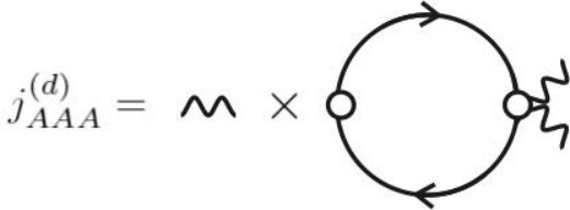 Figure 1
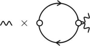 Figure 2
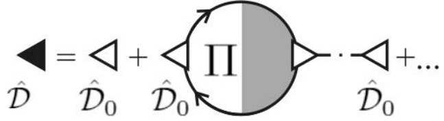 Figure 3
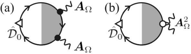 Figure 4
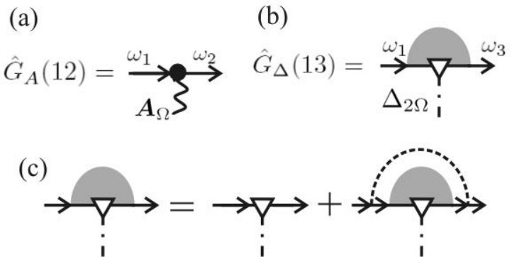 Figure 5
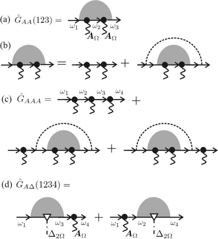 Figure 6
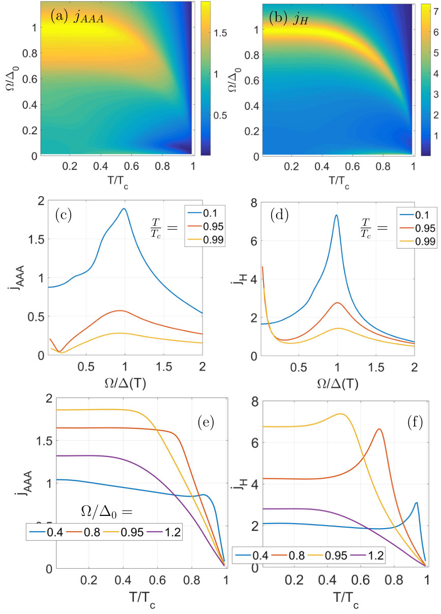 Figure 7
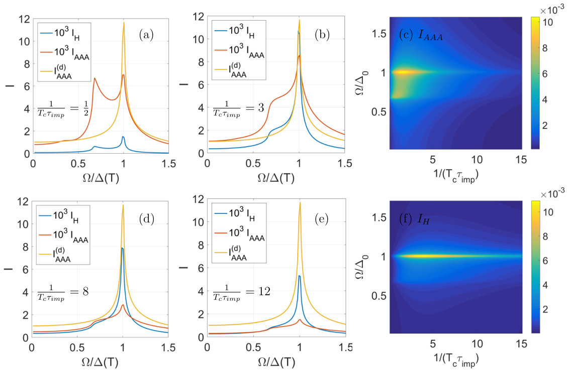 Figure 8
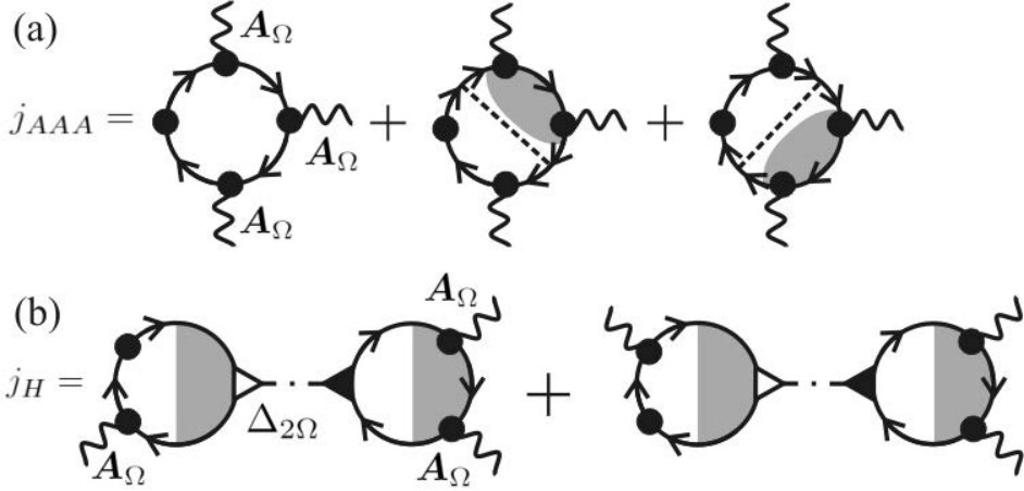 Figure 9
Peer Reviews
No public reviews on file for this paper yet. If you reviewed it on a platform where reviews are public (OpenReview, ICLR, NeurIPS, ICML), you can paste yours below so the community can read it here.
Videos
No videos yet. Explain this paper in a talk, walkthrough, or lecture? Add one.
Nonlinear electromagnetic response and Higgs mode excitation in BCS superconductors with impurities
Mikhail Silaev
Department of Physics and Nanoscience Center, University of Jyväskylä, P.O. Box 35 (YFL), FI-40014 University of Jyväskylä, Finland
Abstract
We reveal that due to the presence of disorder oscillations of the order parameter amplitude called the Higgs mode can be effectively excited by the external electromagnetic radiation in usual BCS superconductors. This mechanism works for superconductors with both isotropic s-wave and anisotropic, such as d-wave, pairings. The non-linear response in the presence of impurities is captured by the quasiclassical formalism. We demonstrate that analytical solutions of the Eilenberger equation with impurity collision integral and external field drive coincide with the exact summation of ladder impurity diagrams. Using the developed formalism we show that resonant third-harmonic signal observed in recent experiments is naturally explained by the excitation of Higgs mode mediated by impurity scattering.
I Introduction
Nonlinear electromagnetic responses are ubiquitous in superconducting systems and have attracted interest for many years Gor’kov and Eliashberg (1968); Gorkov and Eliashberg (1968); Amato and McLean (1976); Gorkov and Eliashberg (1969). External field with the frequency produces several important second-order corrections to the superconducting order parameter . The zero-frequency change of leads to the critical temperature and critical current enhancements Ivlev and Eliashberg (1971); Eliashberg (1970); Tikhonov et al. (2018) known as the microwave stimulation of the superconducting state. The time-dependent corrections to at the frequency produce the current oscillating with frequency Gor’kov and Eliashberg (1968) . This effect called the third harmonic generation (THG) has been observed experimentally in microwaves and explained with the help of the time-dependent Ginzburg-Landau theory Amato and McLean (1976).
Recently the terahertz (THz) spectroscopy of superconducting state has become experimentally available Beck et al. (2011, 2013); Matsunaga and Shimano (2012); Matsunaga et al. (2013, 2014); Giorgianni et al. (2019). This range of frequencies is especially interesting since it overlaps with the typical gap sizes in low-temperature superconductors like NbN. Thus measuring nonlinear responses in THz domain allows for probing dynamics of the order parameter amplitude Matsunaga et al. (2013, 2014) predicted to feature oscillations with an eigen frequency where is the the gap at a given temperature Volkov and Kogan (1974); Kulik et al. (1981); Barankov et al. (2004); Barankov and Levitov (2006). By analogy with the Higgs bosonHiggs (1964) in particle physics this type of collective excitation in condensed matter systems is called the Higgs modeVarma (2002); Podolsky et al. (2011); Pashkin and Leitenstorfer (2014); Volovik and Zubkov (2014); Pekker and Varma (2015). The order parameter amplitude oscillations excited by the short optical pulses has been observed in several pump-probe experiments Matsunaga et al. (2013, 2014). Recent measurements report the evidence of resonant Higgs mode excitation in the THG component of the THz signal transmitted through the superconducting plateMatsunaga et al. (2014, 2017). Earlier the amplitude modes have been observed by Raman scattering in superconductors with charge density wave order Sooryakumar and Klein (1980); Littlewood and Varma (1982); Grasset et al. (2018a, b) and by the nuclear magnetic resonance in superfluid 3He Paulson et al. (1973); Lawson et al. (1973); Zavjalov et al. (2016).
Despite the significant experimental advances, theoretical understanding of high-frequency non-linear properties in superconductors is still lacking. Numerical simulations presented in several works consider strongly non-equilibrium regimes without any disorder Krull et al. (2014); Papenkort et al. (2008); Fauseweh et al. (2017) and have to attribute rather large wavevector to the radiation field in order to obtain the sizable coupling with the order parameter. At the same time perturbative calculations of nonlinear responses reveal several important limitations imposed by the absence of impurity scattering. The order parameter modulation by the external radiation was studied in the pioneering work of Gor’kov and Eliashberg Gorkov and Eliashberg (1968) who considered the electron-photon coupling linear by the vector potential . The contribution of such terms to the order parameter modulation at the frequency is described by the second-order diagram in Fig.1a. Here current vertices describe the linear coupling to the external field. This contribution disappears the absence of impurity scatteringGorkov and Eliashberg (1968). One can think of this as a consequence of the Galilean invariance featured by the superconducting condensate. Indeed switching to the moving frame can eliminate the condensate velocity induced by external field. In the moving frame the order parameter amplitude remains unaffected thus coinciding with that of the stationary condensate. Therefore, in order to perturb the amplitude through the linear electron-photon coupling terms the Galilean invariance should be broken either by the spatially-inhomogeneous field or the inhomogeneous potential which can naturally related to the presence of impurities.
Based on these arguments at zero or negligibly small wave vectors the Higgs mode excitation Tsuji and Aoki (2015) and non-linear responseCea et al. (2016) in the absence of impurities are possible only through the electron density modulation generated by the term in the Hamiltonian. The corresponding density vertices are similar to those which determine Raman scattering in superconductors Abrikosov and Falkovsky (1961); Abrikosov and Genkin (1974); Sooryakumar and Klein (1980); Abrikosov and Falkovsky (1988); Falkovsky (1993). The perturbation of the order parameter due to such coupling is shown by the diagram in Fig.1b. However, this contribution to vanishes within the Bardeen-Cooper-Schrieffer (BCS) model of superconductivity and becomes non-zero only due to the various extensions Tsuji and Aoki (2015); Cea et al. (2016); Matsunaga et al. (2017).
The prediction of negligible Higgs mode generation in BCS superconductors Cea et al. (2016) has been in contrast both to the recent THz probesBeck et al. (2013, 2011); Matsunaga et al. (2014, 2013); Matsunaga and Shimano (2012); Katsumi et al. (2018); Matsunaga et al. (2017) and earlier microwave experimentsAmato and McLean (1976) where significant radiation-induced oscillation have been observed. Here we resolve this controversy and show that previous theoretical conclusions about the non-linear response of superconductors are drastically altered in the presence of disorder. We consider the arbitrary amount of impurity scattering treated within the self-consistent Born approximation. The calculations are implemented using both the diagrammatic technique and quasiclassical Eilenberger theory formalism Eilenberger (1968) and the agreement between these two approaches is demonstrated. We show that in the presence of disorder the non-linear process shown in Fig. 1a provides quite an effective generation of the Higgs mode which shows up through the resonant THG in agreement with several recent experiments.
In the diffusive limit typical for the superconducting thin films our findings confirm that the resonant third-harmonic generation at the frequency observed in Matsunaga et al. (2014) is determined solely by the Higgs mode generation. This result is in sharp contrast with the system without impurities where the Higgs mode generation is negligible and the resonant contribution comes from the other source Cea et al. (2016, 2018). It agrees qualitatively with the studies of linear Higgs mode generation in diffusive current-carrying superconductorMoor et al. (2017); Nakamura et al. (2018).
II Formalism
II.1 General approach
We describe the interaction of electrons with electromagnetic field using the following Hamiltonian which contains two qualitatively different terms Abrikosov and Genkin (1974); Abrikosov and Falkovsky (1988); Falkovsky (1993)
[TABLE]
where is the band velocity, and are the electron mass and charge.
Here we introduce the notation for the Pauli matrices in Nambu particle-hole space. In the diagrammatic representation the perturbation term linear in the external field amplitude is described by the current vertex with attached single external field line. Such current vertices determine diagrams of the type shown in Fig.1a. The term quadratic by the external field produces radiation-induced electronic density modulation. Thus light-matter coupling is described by diagrams with density vertices such as shown by the open circles in Fig.1b.
The charge current and order parameter as functions of the at imaginary time are given by
[TABLE]
where is the imaginary time Green’s function (GF), is the pairing constant, is the projection operator. It will be convenient to use also the frequency representation which can be defined as . In this representation the self-consistency relation can be written as , where is the order parameter vertex which appears first in the diagrams in Fig.(1). The algebraical expression for reads
[TABLE]
The stationary propagators depend only on the frequency corresponding to the relative time . In disordered superconductors with arbitrary amount of point-like impurity scatterers treated within the self-consistent Born approximation propagators are given by (Abrikosov et al., 1963)
[TABLE]
where is the deviation of the kinetic energy from the chemical potential and are the Pauli matrices in Nambu space. We denote and .
The propagator (7) is averaged over the randomly disordered point scatterers configurations. It is parametrised by the scattering time , where is the normal metal density of states at the Fermi level, is the impurity potential strength and is the density of impurities.
We are interested in the non-linear contribution to the current determined by the diagrams in Fig.2 where the coupling to the electromagnetic field is determined by the vector current-type vertices. Such diagrams are generated by the perturbation potential given by Eq.(2). As we see below the contribution of such diagrams to the measurable quantities is captured by the quasiclassical Eilenberger equations Eilenberger (1968). We assume here that all external field lines have the same time dependence , so that diagrams in Fig.2 yield the third harmonic response of the current .
The diagrams shown in Fig.(2a) determine the current generated by the direct coupling to the external field through the current vertices. Dashed lines correspond to impurity scattering averaged over the random disorder configuration. Analytically one should integrate over the input/output momentum the content between the dashed line start and end points as well as multiply the result by the factor . The shaded regions show impurity ladders discussed in detail in Sec.IV.2.
Besides the direct coupling to external field equally important is the third-harmonic generation by the current determined by the order parameter modulation . Taking into account that is generated by external source according to the diagram in Fig.1a the current can be represented by the third-order response diagram in Fig.2b. This contribution is of the special interest since as we will demonstrate its frequency dependence contains the information about the Higgs mode, that is the resonant enhanceable of the order parameter oscillations amplitude at . Technically the resonant Higgs mode contribution is determined by the polarization operator which modifies the gap function vertex shown by the filled triangle in Fig.(2b). This vertex yields the order parameter coupling to the external source such as the second-order correction of the GF by the electromagnetic field discussed above. The diagrammatic representation of the order parameter vertex with polarization bubble insertions is shown in Fig.(3). Note that it contains impurity scattering corrections, both as the self-energies modifying individual propagator lines and the ladder dressing the vertex.
Previously, it has been shown that in the the absence of impurities the contribution of diagrams with current vertices to the order parameter modulation disappears Gorkov and Eliashberg (1968); Tsuji and Aoki (2015); Matsunaga et al. (2014); Cea et al. (2016). In this case the only non-zero contribution is given by the diagrams with density vertices shown in Fig.4. Below we compare the contributions of these diagrams to obtain the threshold impurity concentration when the paramagnetic diagrams start to dominate.
II.2 Quasiclassical theory
In general it is believed that the quasiclassical approximation introduced by Eilenberger Eilenberger (1968) takes into account all diagrams with current vertices shown in Fig. (2) but neglects the ones with density vertices. Technically this happens because the terms in the Hamiltonian generically drop out from the quasiclassical equations. However, previously there has been done no direct comparison of the results given by quasiclassical theory with those obtained from diagrams describing coupling to the external field in the presence of impurity scattering. We will implement this check and demonstrate the summation of diagrams with impurity ladders give the same results as the quasiclassical calculation implemented according to the formalism described below.
The quasiclassical propagator is defined as
[TABLE]
In the imaginary time domain is determined by the Eilenberger equation Eilenberger (1968)
[TABLE]
Here we denote the commutators and the convolution is given by . The angle-averaging over the Fermi surface is given by . The current and order parameter are given by
[TABLE]
where and is the Fermi velocity which is the band velocity at the momentum equal to the Fermi momentum . The quasiclassical equations are supplemented by the normalization condition .
Dirty limit: Usadel theory. In the dirty limit the calculations can be significantly simplified using the Usadel equation formalismUsadel (1970). The key idea of this approximation is to represent the GF as the superposition of isotropic and anisotropic parts. For the validity of Usadel theory it is required that the anisotropic part is small which is satisfied in the diffusive limit. Then using the normalization condition one obtain get the Usadel equation for the isotropic component which reads (we omit angular brackets)
[TABLE]
where the self-energy describes coupling to the electromagnetic field, the the diffusion coefficient is and conductivity is .
III Quasiclassical calculations
First, we obtain time-dependent perturbations of the order parameter and the third-order current response using the Eilenberger theory for quasiclassical propagators. In the Sec.IV these results will be confirmed by the direct summation of impurity ladder diagrams with current-type vertices describing the light-matter interaction.
III.1 Nonlinear response: direct light-matter interaction
We start with calculating corrections generated directly by the time-dependent vector potential. Corrections due to the order parameter oscillations which contain the Higgs mode contribution are considered below in Sec.III.2. In the presence of the oscillating external field we can find the solution of Eilenberger equation (10) in the form of expansion by the orders of as follows
[TABLE]
where we introduce the shortened notation to define the frequency dependence such as and the shifted Matsubara frequencies , , , . The zeroth-order solution given by the unperturbed propagator given from Eqs.(7,9)
[TABLE]
where . The expansion terms in Eq.(16) can be found in the form where momentum direction dependence is explicitly defined
[TABLE]
where we denote and .
The impurity collision integral disappears for the isotropic parts of the propagator, so that we have in the first-order , in the second-order and for the third-order correction . Then we obtain a chain of equations to determine corrections driven by the direct coupling to the vector potential. The equation for the first-order correction reads
[TABLE]
where we introduce the notation and . The second order correction is
[TABLE]
The equation for has the similar form with the replacements in the right hand side. And finally the equation for the third-order correction is
[TABLE]
The solution of above equations reads as follows. The first-order correction is given by
[TABLE]
The isotropic second-order correction is given by
[TABLE]
and the anisotropic part is obtained by the replacements in the right hand side of Eq.(26). Finally, the third-order correction is given by
[TABLE]
As discussed below in Sec.III.4 in order to use solutions (28) for the numerical calculation it is necessary to convert them into the form which does not have the factor in the denominators. This can be done with the help of normalization condition which yields the following relations for the corrections
[TABLE]
The commutation relations for and are obtained by substituting these functions instead of and to the relation (32,33), respectively. As the consistency check, one can prove by the direct calculation that the solutions (26,28) satisfy Eqs.(32,33). With the help of these relations one can rewrite Eq.(28) in the form suitable for numerics as described in the Appendix A. Using this form it is also possible to derive the diffusive limit consistent with the results given directly by the Usadel equations as discussed in Sec.V.4 and in the Appendix B.
III.2 Higgs mode contribution to the nonlinear response
Besides corrections to the GF induced directly by the coupling to vector potential we need to take into account the nonlinear current induced through order parameter oscillations. This process is depicted by the diagrams shown in Fig. 2a. First, let us calculate the current generated by the vector potential combined with the order parameter oscillating with the frequency which we denote as . We can find the corresponding solutions of Eilenberger equation in the form
[TABLE]
We use a similar approach to solve the chain of equations for corrections as in the previous section. Then the obtained first- and second-order solutions read
[TABLE]
where the first-order correction due to the vector potential is given by the Eq.(25). Note that the correction induced by the order parameter oscillations is completely isotropic and therefore is not affected by the impurity scattering collision integral. From this one can immediately conclude that the polarization operator which determines the Higgs mode is not sensitive to the disorder.
As discussed below in Sec.III.4 in order to use the solution (38) for the numerical calculation of the analytical continuation it is necessary to convert it into the form which does not have the factor in the denominator. This can be done with the help of normalization condition of the quasiclassical GF. For the corrections it yields
[TABLE]
One can check by the direct calculation with the certain analytical effort that the solutions (37,38) satisfy the conditions (41,42). Then, using these relations it is possible to convert (42) to the required form as described in the Appendix A.
The correction is the basic building block to calculate the Higgs mode-related current according to the diagram in Fig.2b. In order to obtain as the third-order response to the external field we need to calculate the order parameter amplitude excited in the second order by as shown by the diagram in Fig.1a. This can be done in two steps described below.
External perturbation of the order parameter. First, from the diagram in Fig.1a we find the source, that is the time-dependent order parameter induced directly by the external field. The amplitude can be found using the isotropic second-order correction for the GF calculated above (26)
[TABLE]
Polarization operator Second, to find the order parameter amplitude driven by the external source we need to take into account the polarization corrections given by the diagrammatic series shown in Fig. (3). Thus the renormalized order parameter vertex denoted in Fig.(3) by the filled triangle is related to the bare one as . Here is the polarization operator given by the single bubble in Fig. 3. Thus the total order parameter perturbation is related to the external source as
[TABLE]
Previously, the polarization operator has been calculated in the clean limit Tsuji and Aoki (2015); Cea et al. (2016). In the presence of impurities the diagram summation becomes more complicated because besides the modification of propagator lines we need also to take into account the impurity ladders. However, as shown below in result the expression for remains the same as in the clean limit.
Instead of the direct diagram summation it is much faster to calculate the polarization operator in the presence of disorder within the quasiclassical formalism. Let us assume that there is an external driving term in the gap function given by . Then in the Eilenberger equation we have the source . Besides that there is a response of the order parameter which we denote . Then the amplitude of the total off-diagonal driving term in the Eilenberger equation is . Then we can use this amplitude instead of in the expression (37) for the corresponding correction to the propagator. The self-consistency equation yields
[TABLE]
where we denote as before and . Taking into account that the expression for polarization operator (45) can be transformed to
[TABLE]
The analytical continuation of this expression to real frequencies as explained in Sec.(III.4) yields the result coinciding with the one obtained previously in the clean limit Volkov and Kogan (1974); Kulik et al. (1981); Littlewood and Varma (1982); Tsuji and Aoki (2015); Cea et al. (2016). Note however, that here we have demonstrated that this expression is valid for arbitrary impurity scattering time.
III.3 Total current
Finally we collect expressions for the current given by the diagrams shown in Fig.2
[TABLE]
In order to find the current at real frequency we need to make analytical continuation of Eqs.(47,48) as described in Sec.III.4. In general, this procedure leads to the expressions which can be handled only numerically and in Sec.VI we show the characteristic dependencies of THG current on various parameters. However, in a number of limiting cases it is possible to treat these expressions analytically which we discuss in Sec.V. In the next Sec. we prove that the results of quasiclassical calculations of the non-linear response coincide with those obtained by the summation of diagrams with current vertices in the presence of impurity self-energy and ladders.
III.4 Analytical continuation
In order to find the real-frequency response we need to implement the analytical continuation of Eq.(47,48). These third-order responses are obtained by the summation of expressions which depend on the four shifted fermionic frequencies such as . The analytical continuation of the sum by Matsubara frequencies is determined according to the general rule Kopnin (2001)
[TABLE]
where is the equilibrium distribution function. In the r.h.s. of (49) we substitute in each term and for , denote and , . Here the term with is added to shift of the integration contour into the corresponding half-plane. At the same time, can be used as the Dynes parameter Dynes et al. (1984) to describe the effect of different depairing mechanisms on spectral functions in the superconductor. We implement the analytical continuation in such a way that assuming that the branch cuts run from and .
A special care should given to the differences in the denominators of Eq.(26,28,38) for the second- and third-order responses. When analytically continued to the real energies and frequencies these combinations become zero for certain energies. Indeed, e.g. for , we have is so that for such energy. Thus, the numerical integration of the expressions that contain combinations like in the denominators is not possible. Fortunately, the expressions (26,28,38) with certain analytical effort can be written in the form which does not contain combinations in the denominators. The procedure of how this can be done using the commutation relations (31,32, 33) and (41, 42) for the second-order corrections and third-order correction , is given in the Appendix A.
IV Diagram summation
It is the goal of this section to demonstrate that corrections given by the diagrams with current vertices can be calculated using quasiclassical approximation introduced in the previous section. For this purpose we consider impurity ladder diagrams for corrections up to the third order in external field and use them to derive equations for the corresponding momentum-integrated propagators introduced according to Eq.(9).
IV.1 First-order corrections
Let us start with the simplest diagrams for the first-order corrections induced by the interaction with external field through the current-type vertex and by the order parameter modulation as shown in Fig.(5).
We aim to demonstrate the general approach for deriving equation for the momentum-integrated propagators using the simplest diagram shown in Fig.5a. Let us introduce the notation
[TABLE]
The key idea of the derivation of the simplified equation for is to use the following trick. Let us multiply the function by from the left and by from the right, subtract the results and integrate by . We use that Eq.(7) yields the relations and , where . Then we eliminate off-shell contributions in the momentum integrals to express the result through quasiclassical propagators
[TABLE]
where we introduce the notation . The obtained expression coincides with the r.h.s. of the Eilenberger Eq.(21) for the correction . Next let us derive the l.h.s. of the equation for . Using the diagram Fig.5a we get that . Then, integrating by we obtain the equation to determine coinciding with Eqs.(18, 21).
Let us now consider the momentum integrated correction
[TABLE]
where is given by the more complicated diagram Fig.5b with ladder insertion. Following the procedure described above we get the r.h.s. of the equation for in the form similar to (51). To obtain the l.h.s one needs to use the diagrammatic equation Fig.(5c). Using the fact that does not depend on the momentum direction we write this equation in the algebraic form as follows
[TABLE]
From these equations we obtain . Then terms with impurity scattering in l.h.s. and r.h.s. appear to be exactly the same. In result we recover the quasiclassical equation for with the solution Eq.(37) which is not sensitive to impurity scattering.
IV.2 Second-order correction
In this section we calculate the basic element of the nonlinear response diagrams Fig.2, that is the second-order correction modified by the impurity ladder as shown in Fig.6a. We denote the frequencies , , , .
The correction can be though of as a result of the second-order electron-photon interaction process. It is determined by the equation shown diagrammatically in Fig.6b. Due to the presence of two current vertices the angle average associated with the dashed impurity line produces non-zero result. The corresponding integral equation for reads
[TABLE]
where we denote the angular average and the momentum-integrated GF . From the Eq.(54) we can obtain equation for the momentum-integrated GF . Using the same method as described above in Sec.IV.1 we get the equation for which reads as
[TABLE]
Using the ansatz (19) we get from here Eq.(26) for the components and .
IV.3 Third-order correction
The third-order correction to the GF is determined by the diagram shown in Fig. 6c . The corresponding analytical expression reads
[TABLE]
The straightforward calculation of is rather lengthy. However, it is possible to show that the momentum-integrated function satisfies Eilenberger Eqs. (23,24). The key idea of this derivation is to use the same trick as introduced above in Sec.IV.1 to rewrite the diagrammatic equation in terms of the quasiclassical propagators. First, we multiply Eq.(56) from the left by , from the right by and then subtract the results in the same way as given by the Eq.(51) to obtain the r.h.s. of the Eilenberger equation in the form
[TABLE]
The l.h.s. of the resulting equation can be expressed in terms of the quasiclassical propagators directly from Eq.(56). In this way we obtain
[TABLE]
where are given by the Eqs.(29,30). Using the ansatz (20) we get from Eq.(58) the solutions for components (28).
IV.4 Corrections due to the Higgs mode
Correction to the GF generated by the combined action of the vector potential and the time-dependent order parameter is given by the diagram in Fig.6d. This perturbation determine the non-linear current which is sensitive to the excitation of the Higgs mode as shown by the diagram in Fig.2b. As before we are interested in the momentum-integrated function because it determines the correction to the current. Treating the diagram Fig.6d using exactly the same procedure as above we arrive to the equation for obtained directly from the Eilenbeger formalism. Its solution is given by the Eq.(38).
V Limiting cases and estimations
V.1 Normal state or very high frequencies
First, let us check that in the normal state the third-harmonic response disappears. This can be seen from the analytical continuations of the Eq. (47) for because the Higgs mode-related part does not exist in the normal state. Let us introduce the condensed notation e.g. . In the normal state . Besides that we have and so that the sum , that is does not depend on energy.
Then for the third-order corrections given by Eqs.(28) one can see that . Moreover, . The same relations are true for . Due to this relations, the contributions from different branch cuts (49) in the expression for the normal state current cancel identically.
Note that for the frequencies the effect of superconducting correlations disappears, so one can consider the system as normal metal. Hence the non-linear response vanishes in this high-frequency limit. This is the reason why diagrams with current vertices can be neglected e.g. when studying Raman response where the frequencies associated with single external lines are assumed to be rather large.
V.2 Absence of impurities
Previously it has been noted that in the clean limit, in the spatially homogeneous case and finite frequency the order parameter amplitude is not affected by the irradiation Gorkov and Eliashberg (1968). In that work by Gor’kov and Eliashber only the contribution of diagrams with current vertices has been taken into account. Under the same assumptions non-linear current response also disappears. Here we check our general results for consistency against this limiting case of .
Order parameter perturbation. First, let us look at the second-order corrections which determine perturbation of the order parameter according to the diagram Fig.1a. In the limit the solutions isotropic second-order correction to GF (26) yields (see Appendix C for details)
[TABLE]
Therefore in the Eq.(43) the sum over frequencies disappears so that
[TABLE]
Now let us consider the contribution of the diagram with density modulation Fig.1b. In this case we obtain
[TABLE]
where . The momentum integral in (61) disappears due to the particle-hole symmetryTsuji and Aoki (2015); Cea et al. (2016) which holds up to the corrections of the order . The same conclusion holds in the presence of impurity scattering which modifies propagators and the density vertex as shown in Fig.1b by the shaded region.
Thus, the contribution of density modulation to the Higgs mode excitation always vanishes due to the particle-hole symmetry. Therefore it has been claimed that the Higgs mode does not contribute to the third harmonic generation Cea et al. (2016, 2018). Below we show that in the presence of impurities the non-zero is obtained within the quasiclassical approximation and does not contain any such small prefactors .
THG current response. Let us now consider expression for the current which in the absence of impurities is determined by the third-order correction given by Eqs.(20). The expression which determined the current can be written as
[TABLE]
where is the function which exact form is rather lengthy and not particularly important. Then due to the Eq.(62) the sum over Matsubara frequencies in the Eq.(47) for current disappears since .
V.3 Transition to the clean limit .
As shown above in Sec.V.2 the finite-frequency contribution of diagrams with current vertices Fig.1a disappears in the absence of impurity scattering and other relaxation mechanisms. The contribution of diagram with density vertices Fig.1b is zero with the accuracy of the particle-hole symmetry near the Fermi level. So that the contribution of Higgs mode excitation to the THG signal is expected to have the negligible amplitudeCea et al. (2016, 2018) as compared to the direct coupling described by the diagram in Fig.4. Thus the polarization dependence of THG signal is expected to be sensitive to the lattice anisotropy. Here we show that the above conclusions can drastically altered in the presence of rather small impurity concentrations, typical for all realistic superconducting samples, especially in thin film geometries. Our goal is to find the threshold value of impurity scattering when the diagrams with current vertices become dominant and so that the quasiclassical theory described in Sec.II.2 is applicable for calculating non-linear properties.
To understand the magnitude of this threshold in this subsection let us analyse the amplitudes in the regime of low frequencies, impurity scattering rates and small temperatures as compared to the critical temperature . In Sec.VI the numerical results with broad range frequency and scattering rate dependencies are presented.
Order parameter perturbation. First, let us estimate the magnitude of the external order parameter perturbation in the presence of weak disorder. The contribution of diagrams with current vertices Fig.1a to the order parameter perturbation can be obtained using solution (26) expanded in the regime
[TABLE]
Then at small temperatures the first term here vanishes upon the integration over while the second term yields the leading order expansion by the scattering rate
[TABLE]
Thus the Higgs mode amplitude perturbation driven by the linear electron-photon coupling terms in the Hamiltonian is non-zero for the finite concentration of impurities.
THG current response. At non-zero frequencies the current given by diagrams with current vertices Fig.(2) disappears without impurity scattering and other relaxation mechanisms. At the same time the current determined by diagrams with density vertices in Fig.4 remains non-zero. Let us find the threshold value of impurity scattering when the latter contribution can be neglected.
It is convenient to introduce dimensionless amplitudes , of the currents (47,48) determined by the contribution of diagrams with current vertices
[TABLE]
Here is the normalization current density. In the same way, the contribution of the density modulation diagram in Fig.4 can be written as in terms of the dimensionless amplitude
[TABLE]
Then the dimensionless amplitude is given by
[TABLE]
Hence from the Eqs.(69,65) the ratio of different contributions to the current can be expressed through the ratio of dimensionless amplitudes as follows
[TABLE]
where the prefactor is determined by and is the Fermi energy. As we mentioned above, in the limit the amplitude disappears while remains finite. However, due to the very small prefactor in Eq.(70) the threshold level of occurs to be quite large.
To understand the magnitude of this threshold let us analyse the amplitudes in the regime of low frequencies, impurity scattering rates and small temperatures as compared to the critical temperature .
Under the above assumption one can obtain the analytical expression for the density modulation-induced amplitude . For small we can replace . So that the current amplitude becomes just .
The calculation of quasiclassical contribution is more involved. Let us implement the Taylor expansion in terms of the frequency and the scattering rate of the Eqs.(26,28). In this way we obtain the leading-order terms
[TABLE]
Since we consider low temperatures, when calculating contributions to the current the frequency summation has to be replaced by the integral, e.g. . Then the first terms in the r.h.s. of expansions (71,72) disappears so we end up with the result
[TABLE]
Thus we get the leading-order contribution to the quasiclassical current amplitude
[TABLE]
where we took into account the relation . Thus from (70) we get the ratio of the density- modulation and quasiclassical currents given by
[TABLE]
Note that Eqs.(74,75) are valid at small frequencies and they also agree with the static limit when . Indeed, in the static limit determines non-linear correction to the Meisser current. This correction can be shown to vanish at in the absence of disorder in agreement with Eq..
Based on the estimation (75) the contribution of diagram with density vertex becomes dominating in the limit determined by the condition
[TABLE]
Taking into account that in usual superconductors like NbN with and the above condition yields . This criterion means that the superconductor should be in the super-clean regime Kopnin and Volovik (1997); Kopnin and Lopatin (1995) defined as . Up to now the only known system where this regime is realizedKopnin and Lopatin (1995); Kopnin and Salomaa (1991) is the superfluid He3 which generically does not contain any impurities. In solid state systems the certain amount of disorder is always present. Besides that in thin films the scattering time is bounded from above by the time of flight of electrons between interfaces. Taking into account that in the clean limit the coherence length is the above criterion means that the film should be thicker than which is much larger than what has been used in experiments Matsunaga et al. (2014); Katsumi et al. (2018); Nakamura et al. (2018). Besides that, typical materials used in THz spectroscopy experiments like NbN superconductors usually have strong intrinsic disorder so the dirty limit is realized there even without taking into account the interface scattering.
Another interesting tendency characteristic for the transition to the clean limit is that the Higgs mode-related current is suppressed much strongly than the other component so that . This can be understood from the expansion b small parameter of the GF correction which determine according to the Eq.(48). In this case the amplitude of the order parameter external perturbation is given by (64), that is it already contains the small parameter . Besides that expanding given by Eqs.(37,38,40) we get
[TABLE]
The first term here vanishes as usual upon the integration by while the second term together with Eqs.(64,44) yields the amplitude of the current . Here we need to take into account the low-frequency asymptotic of the polarization operator which follows from Eq.(45) . The we get the non-linear current generated due to the Higgs mode excitation with the dimensionless amplitude given by
[TABLE]
where at low temperatures . Thus one can see that the suppression of in the transition to clean case is determined by the second order of the small parameter . Therefore in this limit except of the vicinity if the Higgs mode resonance at where the amplitude is enhanced by the factor , where is the Dynes parameter. However, if the impurity scattering is sufficiently weak the direct contribution to nonlinear current dominates for all frequencies. These different regimes are illustrated by the numerical results below in the sectionVI.
Estimations that we provided above rule out the necessity to consider the contribution of density-vertex diagrams to describe the non-linear properties of known superconducting materials. Besides that the thin-film samples used for the non-linear response studies in the THz regime are generically in the dirty regime, because the mean free path is bounded from above by thickness because the surface scattering of electrons mimics impurity scattering. Therefore in realistic superconducting samples where the impurity scattering rate is always above the superclean limit the non-linear response is determined only by the diagrams with current vertices Fig.2. As shown above this means that one can use the quasiclassical approximation with impurity collision integrals which yields major simplification as compared to the direct summation of diagrammatic series. Besides that usually the low-temperature superconductors are in the dirty regime which can be treated within even simpler Usadel theory as discussed in the next section. However, the general solutions we obtain can be applied with some modifications to calculate nonlinear responses in clean materials like the d-wave high temperature superconductors Katsumi et al. (2018) or iron-based superconductors which are in the regime .
V.4 Dirty limit
Previously, non-linear electromagnetic properties of superconductors have been studied mostly in the diffusive system using the Usadel formalism Gorkov and Eliashberg (1968, 1969); Gor’kov and Eliashberg (1968); Eliashberg (1970); Ivlev and Eliashberg (1971); Moor et al. (2017); Tikhonov et al. (2018). The general case with arbitrary impurity concentration has been discussed in the linear response regimeArtemenko and Volkov (1979). Here we present for the first time calculations of the non-linear responses with arbitrary impurity scattering time. Therefore it is important to establish connection with the Usadel theory results which should be obtained from our general expressions in the limit . That is, the isotropic second-order correction which determines the order parameter perturbation and the expression for non-linear current response can be obtained directly from Eqs.(13,14,15) as where
[TABLE]
where we normalize the current by the amplitude . The correction induced by the order parameter oscillation is given by Eq.(37) and does not depend on the impurity scattering rate. In the Appendix (B) we demonstrate that the same expressions follow from the general Eqs.(26,47) as the leading term expansions by the small parameter .
VI Numerical results and discussion
Analytical estimations in previous section are obtained at small frequencies . To understand the full frequency dependencies we implement the numerical calculation using the analytical continuation procedure explained in Sec. III.4. At first, our aim is to compare the dimensionless amplitudes of the three contributions to the current , and for different values of the parameters. The results are presented in Fig.7 for different values of the scattering rate varying between the clean and dirty regimes. Here we consider the regime of small temperatures and the Dynes parameter is . These plots confirm qualitative conclusions made above. In the clean case (Fig.7a) the Higgs contribution is much smaller than the direct coupling one . This is despite the fact that Higgs mode contribution is resonant and its maximal value scales like . The contribution also has peaks both as and although their amplitude does not diverge with . The origin of these peaks is the BCS density of states singularity at the energy . The external radiation at frequencies causes transition between these states with the enhanced probability due to the large density of states.
With increased scattering rate the general amplitude of the Higgs mode contribution rises so that its maximal value becomes much larger than the direct contribution. For the considered value of Dynes parameter this happens at rather large scattering as shown in Figs.7d,e. At such parameters which means that if one recalls the overal factor in front of the density modulation current (70). The non-resonant peak in at remains although the one at is eliminated by the impurity scattering. The overall dependencies of and on frequency and scattering rates as shown in 7c,f. One can see that first they increase with but then start to decrease. We discuss the regime with large scattering rate below using the diffusive limit approach .
In thin-film NbN samples used for the non-linear response measurement the amount of scattering is typically rather large. Therefore we consider the diffusive limit below using the Usadel theory results from Sec.V.4 to calculate non-linear currents. Besides that since NbN has strong electron-phonon coupling Matsunaga et al. (2017) resulting in the enhanced inelastic relaxtion we use larger value of Dynes parameter as compared to the previous example. The results for temperature and frequency dependence of currents and are shown in Fig.8. As one can see in Fig.8a,b both currents and have peaks at . However, the peak value of Higgs contribution is several times larger. It occurs when the denominator in Eq.(44) reaches it minimal value of . So the Higgs-mode related part of non-linear current has the same maximal amplitude as compared the part. These estimation agrees with the numerical result in Fig.8c,d.
For higher values of the Dynes parameter which can mimic the enhanced inelastic relaxation in superconductors with strong electron-phonon interaction like NbN Matsunaga et al. (2017) the resonant Higgs peak broadens and decreases. This tendency is illustrated in Fig.8. The broadened peaks featured by the temperature dependencies of at fixed frequencies (Fig.8f) are similar to those obtained in the experiment Matsunaga et al. (2014). At the same time the dependencies of in Fig.8e show no peaks at all.
As we discussed above, the presence of impurities triggers the non-linear response and Higgs mode generation. However, as one can see from the sequence of the plots in Fig.7c,f above certain threshold scattering rate the amplitudes and start to decrease with decreasing . This agrees with the diffusive limit results Eqs.(80, 81) where the currents are determined by the amplitude has an additional small parameter as compared to the prefactor in (68) so that . At the same time the density modulation-related current is not sensitive for disorder and therefore should dominate in the very dirty system as well as in the very clean one. Thus comparing with the prefactor in Eq.(68) we obtain that in the diffusive limit is negligible as long as and start to dominate in the opposite case, that is close to the localization threshold.
The technique developed in the present work for the arbitrary scattering rates can be applied as well to study Higgs mode generation in non-trivial superconductors like those with the d-wave symmetry of the order parameterKatsumi et al. (2018). Within quasiclassical formalism such states are described with the help of the anisotropic pairing constant . Here and are the angles corresponding to the momenta of interacting electrons. Correspondingly the order parameter acquires momentum dependence which should be taking into account when solving the Eilenbeger equation in d-wave superconductor. With that one can see that in the absence of impurities the same limitations on the non-linear response pertain as for the s-wave superconductor. That is, in the completely pure system the second-order electron-photon coupling through the linear terms in the Hamiltonian (2) does not excite Higgs mode and does not produce any THG signal. The presence of impurities certainly helps the situation although their effect is a bit more tricky than in the isotropic s-wave considered here. However since d-wave pairing can be found only in the clean regime one can expect that the amplitude of Higgs mode contribution should be strongly suppressed according to the Fig.7a. However, to figure out the resulting amplitude it is necessary to figure out the value of Dynes parameter which can be much smaller than in low-temperature superconductors thus allowing for large peaks even in the clean system. At the same time we don’t expect the direct coupling current to feature pronounced peaks because of the lack of the density of states singularities in the d-wave superconductor. Thus the influence of impurities on the collective modes in superconductors with non-trivial pairing is potentially very interesting although its detailed study is beyond the scope of the present paper.
Another interesting direction which can be addressed using the formalism developed by us is the nonlinear response and generation of collective modes in multiband superconductors like MgB2 and iron-pnictide compounds. Here in addition to the impurity scattering important effects can be related to the interband tunnelling of quasiparticles and Cooper pairs which should significantly affect non-linear response. With that we can address recent experimental results on the THz pump-probe experiments with MgB2 Giorgianni et al. (2019).
VII Conclusions
We have studied non-linear electromagnet response of superconductors with the amount of disorder varying between the completely pure limit and the dirty regime. The impact of our study is threefold. First, it it demonstrated that the quasiclassical approximation allows for the correct description of the non-linear effects in superconductors coupled to the external electromagnetic field. Propagators obtained by solving quasiclassical Eilenberger equation with the impurity collision integral coincide with those obtained by the direct summation of diagrams with current vertices taking into account the impurity self-energies and ladders.
Second, we demonstrated that effective Higgs mode excitation is possible in usual BCS superconductors without any extensions of the model suggested in previous works. We show that the contribution of diagrams with current vertices start to dominate over the density-modulation related processes for the level of disorder above the extremely weak superclean threshold. Since the superclean regime is hardly realizable in experiments our results provide the basis for the analysis of non-linear responses in realistic superconducting samples to describe the pump-probe or the THG generation experiments in the broad range of frequencies. The same conclusion holds for compounds with unconventional pairing such as the d-wave cuprates Katsumi et al. (2018) or multiband superconductorsAkbari et al. (2013). Theory suggested in the present paper can be applied to analyse the recent data on the Higgs mode in a d-wave superconductorKatsumi et al. (2018) and the collective mode in MgB2 Giorgianni et al. (2019). In general the impurity scattering determines collective mode excitation in superconductors with both the s-wave and non-trivial pairings and should modify the Higgs mode spectroscopy approach which has been suggested recentlyFauseweh et al. (2017)
Third, we have demonstrated that in the diffusive regime which is typical for thin-film superconducting samples used for recent THz measurements the resonant contribution to THG signal is determined by the Higgs mode excitation thus providing the natural explanation of recent experimentsMatsunaga et al. (2014, 2017). The amplitude of this peak is bounded from above by the Dynes parameter which describes the quasiparticle recombination rate due to the electron-phonon interaction.
VIII Acknowledgements
I am grateful to Lara Benfatto for useful discussions. This work was supported by the Academy of Finland (Project No. 297439).
Appendix A Removing singularities in Eqs.(26,28,38)
Eqs. (26) for the second- and for the third-order (28,38) corrections contain the differences in the denominators. When analytically continued this difference becomes zero for certain energy. Therefore these equations cannot be used directly for the numerical integration along the real energy axis. In order to make them suitable for numerics they Eqs. should be written in such a way to eliminate singular combinations in the denominators.
First, we note that one can simplify the expression for the second-order corrections as follows. Substituting Eq. for the first-order correction into the Eqs. (26,28,29) we can rewrite them as follows
[TABLE]
[TABLE]
where we denote
[TABLE]
With the third-order it requires more effort to get rid of the differences in denominators. First, let us demonstrate how this can be done for the correction that determine the Higgs mode contribution to the current (38). We rewrite it as follows , where
[TABLE]
where . Now we need to treat only the term . In order to do that we note the relation
[TABLE]
Using the commutation relationw (41, 42) we obtain then the expression for without singularity
[TABLE]
Now let us apply the same trick to the corrections . We write them as the superposition of two parts, e.g.
[TABLE]
Using commutation relations (31,32,33) we rewrite expression for in the following form
[TABLE]
that does not have singularities. Expressions for the anisotropic part are similar to Eqs.(90, 92) with the change of by and by .
Appendix B Derivation of the response in diffusive limit
First, in the dirty limit we can find corrections to the propagators directly from the Usadel equation which is a simplified version of the Eilenberger equation. In the frequency domain
[TABLE]
[TABLE]
where we denote again , , , . The solution can be written as (79)
[TABLE]
Taking into account the diffusion coefficient the solution for coincides with obtained from the general expression (26) up to the leading term in .
Within the Usadel theory the current can be calculated using general expression (15) to have the form (80,81)
[TABLE]
Taking the dirty limit for general Eq.(47) that determines the current is more tricky. The leading-order correction in the limit is given by (28). First, from the Eq.(25) we find for the first-order corrects in the limit given by
[TABLE]
Using this relation and the commutation relations we obtain
[TABLE]
Thus from Eq.(28) and Eqs.(90,92) we get
[TABLE]
[TABLE]
We substitute the result (98,99) into the expression for current (47) and use the summation to get the expression for the current which is equal to the Eq.(80).
The dirty limit for Higgs mode-related part of the current can be obtained from Eq.(48,37,38,40) in the similar way as above. Using the relation we obtain
[TABLE]
Thus from Eq.(38) and Eqs.(86, 89) we get
[TABLE]
[TABLE]
Using the summation and the expression for current (48) we get the dirty limit expression for the current (96).
Appendix C Absence of the Higgs mode generation without impurities
Without disorder we get from Eq.(82) the expression which according to Eq.(43) determines the order parameter (82)
[TABLE]
Using the relations
[TABLE]
we get
[TABLE]
Substituting this result into Eq.(103) we get as required by the Eq.(59)
[TABLE]
As explained in the main text since the summation by Matsubara frequencies of this expression yields zero, it yields no perturbation of the order parameter amplitude.
The reference list from the paper itself. Each links out to its DOI / PubMed record.
- 1Gor’kov and Eliashberg (1968) L. P. Gor’kov and G. M. Eliashberg, Sov. Phys. JETP 27 , 328 (1968).
- 2Gorkov and Eliashberg (1968) L. Gorkov and G. Eliashberg, JETP 27 , 328 (1968).
- 3Amato and Mc Lean (1976) J. C. Amato and W. L. Mc Lean, Phys. Rev. Lett. 37 , 930 (1976), URL https://link.aps.org/doi/10.1103/Phys Rev Lett.37.930 .
- 4Gorkov and Eliashberg (1969) L. Gorkov and G. Eliashberg, JETP 28 , 1291 (1969).
- 5Ivlev and Eliashberg (1971) B. Ivlev and G. Eliashberg, Sov. Phys. JETP Lett. 13 , 333 (1971).
- 6Eliashberg (1970) G. Eliashberg, Sov. Phys. JETP Lett. 11 , 114 (1970).
- 7Tikhonov et al. (2018) K. S. Tikhonov, M. A. Skvortsov, and T. M. Klapwijk, Phys. Rev. B 97 , 184516 (2018), URL https://link.aps.org/doi/10.1103/Phys Rev B.97.184516 .
- 8Beck et al. (2011) M. Beck, M. Klammer, S. Lang, P. Leiderer, V. V. Kabanov, G. N. Gol’tsman, and J. Demsar, Phys. Rev. Lett. 107 , 177007 (2011), URL https://link.aps.org/doi/10.1103/Phys Rev Lett.107.177007 .