State graphs and fibered state surfaces
Darlan Gir\~ao, Jessica S. Purcell

TL;DR
This paper introduces an algebraic criterion based on state graphs to determine when checkerboard surfaces of knots and links are fibers, enabling classification of fibering properties for various families, including 2-bridge links.
Contribution
It provides a new algebraic condition to identify fibered checkerboard surfaces directly from state graphs, advancing the understanding of fibering in knot theory.
Findings
Algebraic condition characterizes fibered checkerboard surfaces.
Classifies fibering for families of planar graphs.
Determines fibering for 2-bridge links.
Abstract
Associated to every state surface for a knot or link is a state graph, which embeds as a spine of the state surface. A state graph can be decomposed along cut-vertices into graphs with induced planar embeddings. Associated with each such planar graph is a checkerboard surface, and each state surface is a fiber if and only if all of its associated checkerboard surfaces are fibers. We give an algebraic condition that characterizes which checkerboard surfaces are fibers directly from their state graphs. We use this to classify fibering of checkerboard surfaces for several families of planar graphs, including those associated with 2-bridge links. This characterizes fibering for many families of state surfaces.
Click any figure to enlarge with its caption.
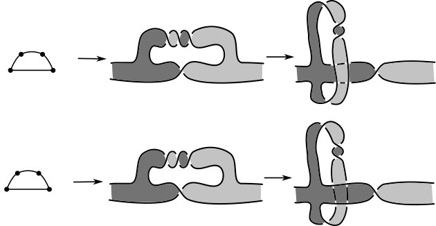 Figure 1
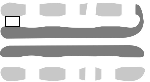 Figure 2
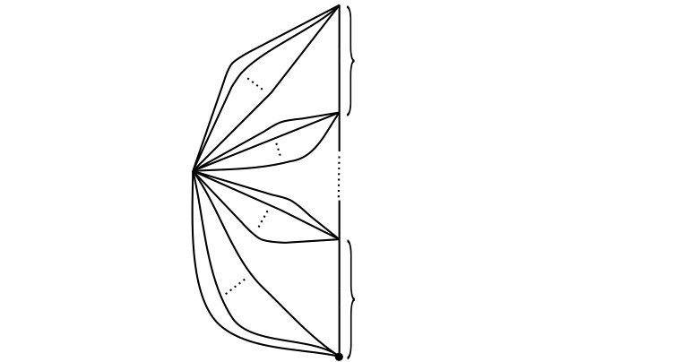 Figure 3
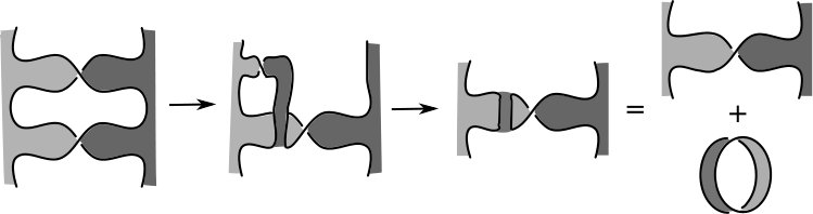 Figure 4
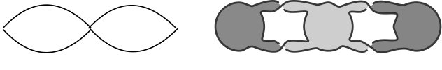 Figure 5
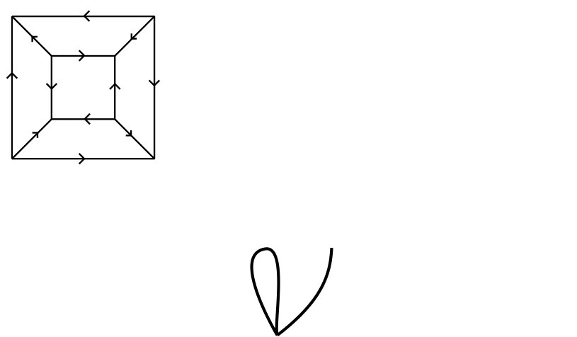 Figure 6
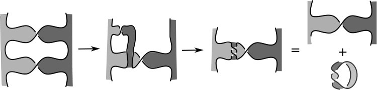 Figure 7
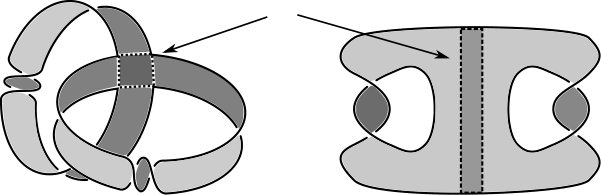 Figure 8
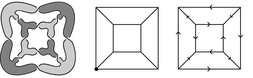 Figure 9
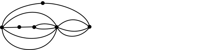 Figure 10
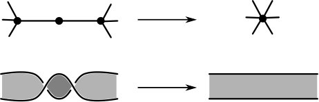 Figure 11
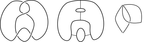 Figure 12
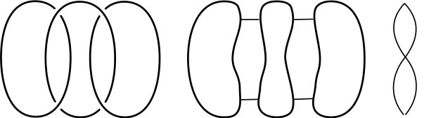 Figure 13
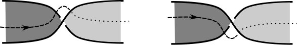 Figure 14
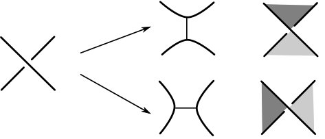 Figure 15
Peer Reviews
No public reviews on file for this paper yet. If you reviewed it on a platform where reviews are public (OpenReview, ICLR, NeurIPS, ICML), you can paste yours below so the community can read it here.
Videos
No videos yet. Explain this paper in a talk, walkthrough, or lecture? Add one.
State graphs and fibered state surfaces
Darlan Girão
and
Jessica Purcell
Abstract.
Associated to every state surface for a knot or link is a state graph, which embeds as a spine of the state surface. A state graph can be decomposed along cut-vertices into graphs with induced planar embeddings. Associated with each such planar graph is a checkerboard surface, and each state surface is a fiber if and only if all of its associated checkerboard surfaces are fibers. We give an algebraic condition that characterizes which checkerboard surfaces are fibers directly from their state graphs. We use this to classify fibering of checkerboard surfaces for several families of planar graphs, including those associated with 2-bridge links. This characterizes fibering for many families of state surfaces.
1. Introduction
Associated to a diagram of a knot or link in the 3-sphere are several embedded spanning surfaces called state surfaces. These arise from a choice of Kauffman state, which were introduced by Kauffman to give insight into the Jones polynomial [21]. The associated surfaces, introduced in [26] and [27], arise naturally as ribbon graphs. State surfaces are known to be related to knot and link polynomials; see for example [4, 7, 18]. State surfaces are also related to the hyperbolic geometry of the link complement for hyperbolic links; see for example [9, 8, 7, 1, 2, 5]. Because of their connections with geometry, topology, and link invariants, these surfaces have recently become objects of much study in knot theory. In this paper, we consider when such surfaces can be fibers.
If we put restrictions on the Kauffman states, there are already results that determine if a state surface is a fiber. For a class of states called homogeneously adequate states, work of Futer [6] and Futer, Kalfagianni, and Purcell [7] shows that the associated state surface is a fiber if and only if a related graph, called the reduced state graph, is a tree. This answered a question of Ozawa [26]. In [7], it is shown that for some special states, fibering is also indicated immediately by the colored Jones polynomial. For other restrictions of state surfaces, the problem of fibering such state surfaces has been considered by Girão [12] and Girão, Nogueira, and Salgueiro [13]. However, we wish to find ways of classifying fibrations of all state surfaces, without restrictions on the Kaufmann state.
The study of fibered knots and links has been ongoing since the early 1960s, introduced by work of Neuwirth [24] and Stallings [29], followed by results of Murasugi [22]. In the 1970s, further work of Stallings [30] and Harer [15] gave insight on constructing fibered knots and links. In the 1980s, Gabai [10] gave a procedure to decide whether an oriented link is fibered, and this has had numerous applications. To date, several results exist that prove that a given knot is fibered. For example, work of Ghiggini [11] and Ni [25] shows that whether or not a knot is fibered can be determined using knot Floer homology. However, we are interested not in whether there exists some fibering of a knot or link, but whether a particular fixed state surface is a fiber. This is not always easily determined even if it is known that a link is fibered; see the discussion below on 2-bridge knots and links.
There do exist examples of knots and links and fixed surfaces for which fibering can be determined immediately from a diagram. These include standard diagrams of pretzel links, due to Gabai [10], and Montesinos knots, due to Hirasawa and Murasugi [17]. Previous results on fibering of state surfaces for restricted states are also along these lines [6, 7, 12, 13]. These are the types of results that we wish to generalize.
The first main result of this paper is Theorem 2.5, which says that whether a state surface is a fiber is completely determined by an associated graph , called the state graph, which can be quickly read from the diagram. In particular, we reduce the problem of determining fibering for a state surface with a complicated embedding into to the problem of determining fibering for checkerboard state surfaces.
The next main result is Theorem 4.2, which gives an algebraic condition that characterizes when a checkerboard state surface is a fiber. In particular, it suffices to prove that a homomorphism is an isomorphism, where the map is read directly from ; see Proposition 4.5. Stallings gave a method to determine whether a homomorphism of free groups is an isomorphism, now called the Stallings folding algorithm [31]. This has had many applications, especially in geometric group theory. By work of Touikan, the algorithm produced runs in almost linear time [32]. We show here that our state graph homomorphisms feed neatly into to the Stallings folding algorithm, and thus we can read whether or not a state surface is a fiber from its state graph in almost linear time.
We conclude the paper by giving several applications, determining many new examples of families of knots and links with fibered state surfaces. One additional result that comes out of this work, which may be of independent interest, is a classification of those 2-bridge link diagrams for which the (bounded) checkerboard surface is a fiber. Recall that a 2-bridge link is determined by a rational number , and the link has several natural diagrams, determined by different continued fraction expansions of (notation described in Section 5). Denote the diagram by . Hatcher and Thurston note that a 2-bridge knot is fibered if and only if it is isotopic to , and the fiber is isotopic to a particular spanning surface [16]. However, the surfaces they describe do not ever have the form of a checkerboard surface. Here, we determine exactly which values of give a checkerboard surface that is a fiber, i.e. isotopic to one of Hatcher and Thurston’s fibered surfaces.
1.1. Organization
In Section 2, we review terminology used in this paper. In particular, we define Kauffman states, state surfaces, and state graphs. With terminology defined, we then state carefully our first result, Theorem 2.5. In Section 3, we review important theorems on fibering due to Gabai and others, and give the proof of Theorem 2.5. In Section 4, the statement and proof of our algebraic characterization of fibering is given, after recalling work of Stallings. Applications are then presented in Section 5. This section includes, for example, a complete characterization of when the bounded checkerboard surfaces of 2-bridge links are fibered, Theorem 5.7.
1.2. Acknowledgements
We thank João Nogueira for helpful conversations, and we thank David Futer for bringing our attention to Stallings folds. The first author was partially supported by Conselho Nacional de Desenvolvimento Científico e Tecnológico (CNPq) grants 446307/2014–9 and 306322/2015–3 and the CAPES Foundation. The second author was partially supported by the Australian Research Council.
1.3. Dedication
While this work was underway, the first author, Darlan Girão, was diagnosed with aggressive cancer, and he died before the paper was complete. Darlan was a wonderful colleague and friend, and he will be missed. This paper is dedicated to his memory.
2. Preliminaries and main results
Given a diagram of a link , at each crossing there are two choices of resolutions for the smoothing of the crossing: an -resolution or a -resolution; see Figure 1. By choosing a resolution at each crossing, we construct a collection of circles, called state circles, which are the boundaries of disjoint disks, called state disks. These state circles induce a decomposition of the plane into connected components that we call regions. Connect the circles by edges labeled or , to indicate a resolved crossing and its resolution, as in Figure 1.
A Kauffman state of a link diagram is a choice of resolution at each crossing of . Given a state , add twisted bands connecting the state disks, one for each crossing, according to the choice of resolution. We thus obtain a surface whose boundary is the link . The resulting surface is called the state surface of . For example, the Seifert surface of an oriented diagram of a link is a particular case of a state surface, where the resolution of each crossing is defined by the orientation of the link components.
The state graph has one vertex for each state disk and one edge for each band defined by the state . We label the edges by or according to the resolution of the respective crossings. Note that the graph has a natural embedding in the surface as its spine. Figure 2 shows an example of a diagram, a Kauffman state, and the corresponding state graph with its associated embedding.
Definition 2.1**.**
We say that a vertex decomposes a graph into components if and contain at least one edge, and and . We also say is a cut-vertex of .
Lemma 2.2**.**
The cut-vertices of a state graph decompose it into a finite collection of planar 2-connected graphs, with planar embeddings determined by the Kauffman state.
This decomposition is illustrated for the example of Figure 2 on the far right of that figure.
It is not hard to see that every state graph admits a planar embedding. However, this embedding may not be isotopic to the embedding associated with the state surface, and so it is not obviously useful from the point of view of analyzing spanning surfaces. The point of Lemma 2.2 is that after decomposing along cut-vertices, the remaining pieces all have a planar embedding induced from the state surface.
Proof of Lemma 2.2.
Suppose each state circle bounds a disk that is disjoint from the diagram of the link; for example this will hold if the state graph has no cut-vertices. The Kauffman state connects these disks by edges labeled or that lie in the plane, and are disjoint from the interiors of the disks. Thus when we collapse each disk to a point, the state graph we obtain remains planar.
So suppose there is a state circle such that disks on both sides meet the diagram. Then this corresponds to a cut-vertex. There must be an innermost such state circle . That is, bounds a disk in the plane such that both and meet the diagram, but all state circles within bound disks disjoint from the diagram. Decompose the state graph along the corresponding cut-vertex. This decomposes the state graph into a graph associated with the outside of and a graph associated with the inside of . On the outside of , there are at most cut-vertices, and so the result follows by induction. On the inside of , all state circles bound disks disjoint from the diagram. But now the state circle also bounds a disk disjoint from the remainder of the diagram. By the previous argument, the graph we obtain by collapsing all these disks to points is planar, with embedding determined by the Kauffman state. ∎
As in Figure 2, the planar graphs determined by Lemma 2.2 may have multiple edges connecting the same pair of vertices, and these edges may be labeled both and . We say that two edges are parallel within the plane if the edges are ambient isotopic in the plane in the complement of all other edges and vertices of the graph.
For multiple edges connecting the same pair of vertices that have the same label ( or ) and that are parallel within the plane, remove all but one such edge. When all such edges are removed, the resulting graph is called the reduced state graph. Note that multiple edges may remain in the reduced state graph, but they will either have distinct labels, or they will not be parallel. Figure 3 illustrates this by example.
Any planar graph with edges labeled and corresponds to a checkerboard surface as follows. For each vertex, take a disk. For each edge, take a twisted band, with direction of twisting determined by the label or ; see Figure 4.
In addition to multiple edges, we may also reduce our planar state graphs by considering consecutive edges.
Definition 2.3**.**
Two edges are called consecutive if they share a vertex and there are no other edges incident at .
Lemma 2.4**.**
If two consecutive edges in a reduced state graph do not have the same label, then the corresponding link and state surface can be isotoped to a simpler link, removing two crossings. On the graph, this corresponds to collapsing the two edges.
Proof.
The simplification is shown in figure 5. ∎
We can now state our first main theorem.
Theorem 2.5**.**
Let be a diagram of a link in with oriented state surface associated to the state . Decompose the corresponding state graph along cut-vertices into planar graphs, and consider the reduced planar graph, with parallel edges with the same label removed. Finally, collapse consecutive edges with distinct labels. Let denote the resulting collection of planar graphs. The surface is a fiber if and only if for each , the associated checkerboard surface is a fiber.
Note that a spanning surface for a link in can only be a fiber if it is orientable; thus we restrict to orientable surfaces in Theorem 2.5. Observe from the definitions that a state surface will be orientable if and only if its state graph is bipartite, so we restrict to bipartite state graphs.
Remark 2.6**.**
By Lemma 2.4, to determine if a state surface is a fiber, it suffices to collapse consecutive edges with distinct labels. But this is done in Theorem 2.5 after the state graph has been decomposed along cut-vertices and reduced. The decomposition and reduction may create new consecutive edges with distinct labels, which can then be collapsed. However, the isotopy of Lemma 2.4 does not extend in general across a cut-vertex, or across multiple crossings corresponding to parallel edges.
Corollary 2.7**.**
Let be diagrams of links in and let be oriented state surfaces associated to the states of the diagrams, respectively. Decompose the corresponding state graphs , along cut-vertices into planar graphs, and for each planar graph component, take the associated reduced graph and remove consecutive edges with distinct labels. Suppose that the reduced planar graphs coming from can be matched in one-to-one correspondence with the reduced planar graphs coming from , by ambient isotopy within the plane via an isotopy preserving labels and . Then is a fiber if and only if is. ∎
We illustrate Corollary 2.7 by an example. In figures 2 and 6 we have two distinct links with given resolutions, each with a single cut-vertex. When we decompose, for each link we obtain two graphs that are cycles with two edges having the same label. The reduced graphs of the decomposition are then a pair of single edges, one labeled and one labeled . Thus the hypotheses of Corollary 2.7 are satisfied, and one is fibered if and only if the other is fibered. In this case, both examples are well-known to be fibered. Notice, however, that the links and the state surfaces are completely different (not homeomorphic).
A Kauffman state is said to be homogeneous if all resolutions of the diagram in each region are the same, and adequate if there are no 1-edge loops. In [6] and [7], it was shown that a state surface associated with a homogeneous, adequate state is a fiber if and only if the reduced state graph is a tree. We obtain the following corollary.
Corollary 2.8**.**
Suppose is a link in with oriented state surface , and suppose the associated reduced state graph is a tree. Then is a fiber.
Proof.
If the reduced state graph is a tree, it decomposes along cut-vertices into a collection of graphs made up of single edges. For each single edge, the associated checkerboard surface is the state surface of a homogeneous state, thus by [6, 7], each is fibered. Then Theorem 2.5 implies the original link is also fibered. ∎
Note that Girão, Nogueira, and Salgueiro also obtained a result that a particular state surface is a fiber if and only if the associated state graph is a tree [13]. However, the converse to Corollary 2.8 is not true. There are examples of states for which the state graph is not a tree, and yet the state surface is still a fiber. We present examples below, such as Example 4.7. These contrast to the results of [6, 7, 13].
3. Murasugi sums and cut-vertices
This section gives the proof of Theorem 2.5. We first recall standard definitions and results from fibered knot theory.
Definition 3.1**.**
The oriented surface in with boundary is the Murasugi sum of the two oriented surfaces and with boundaries and if there exists a -sphere in bounding balls and with for , such that and , where is a -sided polygon (a disk). See Figure 7.
The result concerning Murasugi sum we need is the following, due to Gabai [10].
Theorem 3.2** (Gabai).**
Let , with , be a Murasugi sum of oriented surfaces , with , for . Then is fibered with fiber if and only if is fibered with fiber for . ∎
Lemma 3.3**.**
Let be a state graph embedded in and suppose there is a cut-vertex that decomposes into graphs , . Consider the state surface induced by and the subgraph of , . Then is a fiber if and only if each of and is a fiber.
Proof.
Each vertex of is associated to a disk in the state surface . The fact that is a cut-vertex means that and lie in balls , , with , as required by Definition 3.1. Thus the result follows from Theorem 3.2. ∎
Theorem 3.2 gives a quick proof of the following proposition.
Proposition 3.4**.**
Suppose is a link diagram with oriented state surfaces and associated state graph embedded as a spine in . Decompose the state graph along cut-vertices into planar graphs. Then is a fiber if and only if for each graph in the decomposition of the associated checkerboard surface is a fiber.
Proof.
The graph decomposes along cut-vertices into planar subgraphs by Lemma 2.2. By Lemma 3.3, is a fiber if and only if the state surfaces induced by the are fibers. ∎
3.1. Further decompositions of graphs
To go from Proposition 3.4 to Theorem 2.5, we need to consider reduced graphs. The main tool is the following lemma.
Lemma 3.5**.**
Suppose the state graph has a planar embedding induced from the state surface . Suppose it has multiple edges connecting a pair of vertices, and suppose that those edges are parallel (ambient isotopic) in the plane.
- (1)
If multiple parallel edges have the same label, then is a fiber if and only if the same is true for the state surface corresponding to the graph with all but one of the edges removed. 2. (2)
If two of the parallel edges have distinct labels, then is not a fiber.
Proof.
In both cases, we may use a Murasugi sum to decompose the surface. In the first case, parallel edges with the same label correspond to a Murasugi sum of a Hopf band; see Figure 8. The twisted annulus bounded by a Hopf band is well-known to be fibered.
In the second case, parallel edges with different labels correspond to a Murasugi sum of an annulus; see Figure 9. The untwisted annulus in is well-known not to be fibered. Then the result follows by Gabai’s theorem, Theorem 3.2. ∎
Corollary 3.6**.**
Suppose is a link in with oriented state surface , and suppose the associated state graph has parallel edges with distinct labels. Then is not a fiber.
Proof.
Parallel edges with distinct labels will remain parallel edges with distinct labels after decomposing along cut-vertices. Then the result follows from Theorem 2.5 and Lemma 3.5. ∎
Proof of Theorem 2.5.
By Proposition 3.4, is a fiber if and only if for each graph in the decomposition of its state graph along cut-vertices, the associated checkerboard surface is a fiber. By Lemma 3.5, that checkerboard surface is a fiber if and only if the checkerboard surface associated with the corresponding reduced graph is a fiber. By Lemma 2.4, the checkerboard surface associated with the reduced graph is a fiber if and only if the same is true of the checkerboard surface associated with the graph obtained by collapsing consecutive edges that do not have the same label. ∎
4. Stallings criterion
By Theorem 2.5, we may reduce the task of determining which state surfaces are fibers to considering checkerboard surfaces. To determine which checkerboard surfaces are fibers, we will apply the following theorem of Stallings [30].
Theorem 4.1** (Stallings).**
Let be a compact, connected, oriented surface with nonempty boundary . Let be a regular neighborhood of and let . Let , where is the projection map. Then is a fiber for the link if and only if the induced map is an isomorphism.
As a consequence of Theorem 4.1, we obtain a tool to determine fibering from state graphs:
Theorem 4.2**.**
Let be a state surface with state graph embedded as a spine, and let be a basepoint on . Let , where is the projection map, and let . Then the map uniquely determines a map , and is a fiber if and only if the map is an isomorphism of groups.
Proof.
The graph lies naturally in as a spine, and therefore the inclusion induces an isomorphism . Similarly, there is an isomorphism
[TABLE]
induced by the deformation retraction to , where denotes a regular neighborhood. Deformation retractions (and inclusions) induce the following additional isometries:
[TABLE]
Finally note that we may also assume
[TABLE]
Consider the map
[TABLE]
induced by the following compositions:
[TABLE]
where the first map is the inclusion, the second map is the map , the third map is given by deformation retraction, and the fourth and fifth maps are given by inclusion. Thus the map is an isomorphism if and only if the map in Stallings theorem is an isomorphism, and is a fiber if and only if is an isomorphism. ∎
We call the map in Theorem 4.2 the Stallings map. We need to determine the effect of the Stallings map. We start by considering the form of the complement .
Suppose that a state graph , embedded as the spine of a state surface , is planar with no cut-vertices. Then is a handlebody built as follows.
- •
There is one 0-handle above the plane of projection , and one below.
- •
For each region of , there is a 1-handle running through that region with one end on and the other on .
Lemma 4.3**.**
Suppose that the state graph , embedded as the spine of a state surface , is planar and has no cut-vertices. Suppose that is oriented, so is bipartite, with vertices labeled and , and edges labeled and according to the choice of resolution. Let be a directed arc in that runs over an edge. Denote the 0-handles of by and , as above. Let denote the 1-handle running through the region to the left of the edge (determined by the direction of ), and let denote the 1-handle running through the region to the right. Then the effect of the map , where is the projection map, is as follows.
- (1)
If is a monotonic arc running from a vertex labeled to one labeled over an edge labeled , then runs from to along the 1-handle . 2. (2)
If runs from a vertex labeled to one labeled over an edge labeled , then runs from to along the 1-handle . 3. (3)
If runs from a vertex labeled to one labeled over an edge labeled , then runs from to along the 1-handle . 4. (4)
If runs from a vertex labeled to one labeled over an edge labeled , then runs from to along the 1-handle .
Proof.
If starts on a vertex labeled and runs to one labeled , then begins at and ends at . Similarly if starts at a vertex labeled and runs to one labeled , then begins at and ends at . The 1-handles that meets are determined by the twisting of along the twisted band attached at the crossing of the edge, with twisting in one direction for an edge labeled and in the other direction for an edge labeled . The effects are shown in Figure 10. ∎
Suppose is a state graph that comes out of Theorem 2.5, namely it is planar with no cut-vertices. To determine whether the associated state surface is a fiber, we choose generators for and consider their image under the Stallings map .
Because is orientable, is bipartite, i.e. every closed loop has even length. Label each vertex either by or in an alternating fashion. Label the basepoint in with to obtain a well-defined labeling of vertices of .
The graph divides the plane into regions. The unbounded region is denoted by . The bounded ones are denoted by .
Corresponding to each region , there is a 1-handle with its ends on the 0-handles and , above and below the plane of projection, respectively. Since the basepoint of is labeled , its image lies on . For each bounded region , , define a curve based at as follows. The curve leaves the basepoint and runs monotonically down the 1-handle through the region to the 0-handle . It then runs up the 1-handle through the unbounded region to connect to , and back to the basepoint . Then form a generating set for .
Given a loop based at , its homotopy class in is given by a word in the letters as follows: Starting at , move along acording to the choice of orientation. If crosses a region from above to below, then write the letter . If crosses a region from below to above, then write the letter . Going around once gives a word which represents its homotopy class in . If the region is crossed, then write no letters.
Definition 4.4**.**
The following procedure defines a new labeling on the graph , with labels the letters . Direct each edge from to . If the edge is labeled , assign to the directed edge the letter , where is the region to the left of the directed edge, or if the region to the left is unbounded. If the edge is labeled , assign the letter , where is the region to the right of the directed edge, or if the region to the right is unbounded.
Proposition 4.5**.**
Suppose that the state graph , embedded as the spine of an oriented state surface , is planar and has no cut-vertices. The effect of the Stallings map is as follows. A generator of is represented by a word in the edges of . The image of under is represented by a word in the letters , where each edge contributes a letter as follows.
Consider the labeling of Definition 4.4.
- (1)
If is the label on , and runs along from to , write . 2. (2)
If is the label on , and runs along from to , write . 3. (3)
If is labeled and runs along , write no letters.
Proof.
This follows from Lemma 4.3 and our choice of generators of and defined above. ∎
Corollary 4.6**.**
Suppose that the state graph , embedded in the spine of an oriented state surface , is planar with no cut-vertices, and let denote the generators of as above. Then is a fiber if and only if the group generated by is isomorphic to . ∎
Example 4.7**.**
Consider the link in Figure 11.
The base point is indicated. The labeling of Definition 4.4 is shown on the far right. Let denote generators of as follows. The curve begins at , traverse a path to the boundary of the region , runs counter clockwise around , then traverses the path back to . More specifically, we choose to be the arc given by the lower horizontal edge starting at , we choose to be the arc given by the lower horizontal edge followed by the vertical right-most edge, and we choose to be the diagonal edge with endpoint on . The arcs and are trivial. Following the recipe of Proposition 4.5, we obtain:
[TABLE]
It is possible to see directly that this map is an isomorphism; its inverse given by:
[TABLE]
Therefore the state surface shown is a fiber for the corresponding link.
4.1. Stallings folding
In [31], Stallings describes a procedure that can determine whether a homomorphism of free groups is an isomorphism. See also Kapovich and Myasnikov [20].
Definition 4.8**.**
An edge folding of a directed labeled graph is a new directed labled graph obtained by identifying two edges and of that share the same vertex , and have the same label and the same direction incident to . A directed labeled graph is folded if at each vertex there is at most one edge with a given label and incidence starting (or terminating) at .
A folded graph admits no edge foldings.
Fix a basepoint on a directed labeled graph. The fundamental group of the graph is determined by concatination of paths; group elements are determined by writing words in the labels traversed by a path, where if an edge has label and is traversed in the direction of , we write , and if in the opposite direction, we write . Two words are freely reduced if two labels and never appear consecutively. Note this is a way of representing the fundamental group as a subgroup of a free group; the labeled graph is a covering space corresponding to the subgroup. We call this the group defined on the graph.
The following is straightforward; see [20].
Proposition 4.9**.**
Let and be two directed labeled graphs. If is obtained from by an edge folding, then the two groups defined on the graphs are isomorphic. If is folded, then for any loop in , the corresponding word is freely reduced.
Starting with any graph, perform a sequence of edge foldings, strictly reducing the number of edges, until the process terminates in a folded graph. Touikan showed that there is an algorithm to fold a graph that runs in almost linear time [32].
Corollary 4.10**.**
Suppose is a planar state graph with no cut vertices that is embedded as the spine of an oriented state surface . Suppose is the free group on letters. Let be a directed labeled graph obtained from by the process of Definition 4.4. Let denote the result of after folding. Then the state surface is a fiber if and only if is a rose with petals.
Proof.
The graph encodes the image of Stallings’ map . Stallings folding implies that the graph is a rose with petals if and only if is surjective. Because free groups are Hopfian, this holds if and only if is an isomorphism. The result follows from Theorem 4.2. ∎
Figure 12 shows the folding process applied to the directed labeled graph of Figure 11. Note the fact that the state surface of that example is a fiber now follows from Corollary 4.10.
5. Applications
In this section, we consider some simple graphs and completely classify when they correspond to state surfaces that are fibers.
5.1. The state graph or reduced state graph is a tree
This is the case of Corollary 2.8. We have seen that the state surface is always a fiber.
5.2. The reduced state graph decomposes into cycles
Lemma 5.1**.**
Suppose is a link with state surface . Suppose that the reduced state graph corresponding to is a cycle. Then is a fiber if and only if there are exactly two more edges in the cycle labeled than , or vice versa.
Proof.
Let denote the reduced state graph; the fact that is a cycle means that the (checkerboard) state surface induced by is an annulus. The original state surface , whose state graph may have multiple parallel edges with the same label, is obtained by taking Murasugi sums of Hopf bands with the annulus , as in Lemma 3.5. The graph is a string of consecutive edges. Untwist as in Lemma 2.4, obtaining a new graph for which all edges have the same label. Now consider the Stallings map . Because the surface is orientable, has an even number of edges. We have and . By Proposition 4.5, the image of the generator under is given by , where is the number of edges in , and the sign is positive or negative depending on whether the labels of are or . Note is an isomorphism if and only if . Thus the original state surface is a fiber in this case if and only if has exactly two edges, meaning there are exactly two more edges of the reduced graph that are labeled than those labeled , or vice versa. ∎
Note that the unbounded checkerboard surfaces for pretzel links fall into the class of the surfaces satisfying the hypotheses of Lemma 5.1. Gabai treats these as type III surfaces in [10]. Gabai has more conditions on when these links fiber. However, note that in the cases distinct from Lemma 5.1, the fibered surface is not the given state surface.
5.3. Graphs the shape of a theta and pretzel links
A next simple class of graphs to consider are those that have the shape of a : that is, there are three collections of consecutive edges meeting two vertices; we call each of the three collections of consecutive edges a strand. There will be vertices on the first strand, on the second, and on the third, where either all are even or all are odd to ensure the graph is bipartite. We may also assume, after reducing, that all edges on each strand have the same label. The induced checkerboard state surface will be the bounded checkerboard surface of a pretzel knot with three strands, and crossings on each strand. In fact we may generalize to strands: each strand has vertices, all edges on a strand have the same label, and all the are even or all are odd. Call such a graph a generalized theta graph. The induced checkerboard surfaces are bounded checkerboard surfaces for pretzel links.
The fibering of such checkerboard surfaces has been completely classified. When , this follows from work of Crowell and Trotter [3]. For other values of , partial results were obtained by Parris [28], and independently by Goodman and Tavares [14], and Kanenobu [19]. Their results are summarized and generalized by Gabai [10]. The full result is the following.
Theorem 5.2** (Bounded checkerboard surfaces of pretzel links).**
Let be nonzero integers. The pretzel link determined by crossings has a bounded checkerboard surface that is a fiber if and only if one of the following holds:
- (1)
each or and some . 2. (2)
* for (here is odd).* 3. (3)
* (here is even).*
Corollary 5.3**.**
Suppose a reduced state graph has the shape of a generalized theta graph. Reduce further to remove consecutive edges without the same label. Then the associated checkerboard surface is a fiber if and only if one of the following holds:
- (1)
Each strand has [math] or vertices, and some strand has [math] vertices. All strands with [math] vertices are labeled or are all labeled ; strands with vertices are exactly the opposite (all or all ). 2. (2)
There are an even number of strands, each strand except the last has vertex, all strands except the last alternate being labeled and , and the final strand has any number of vertices with any label or on all edges of the strand. 3. (3)
There are an odd number of strands, each strand except the last has vertex, all strands alternate being labeled and , and the final strand has three vertices.
5.4. Checkerboard surfaces of two-bridge links
We conclude with one final family of reduced state graphs whose fibering we can completely classify: those that arise from diagrams of 2-bridge knots. Essential surfaces in 2-bridge knots were classified by Hatcher and Thurston [16], and they note in that paper that those spanning surfaces that are fibers are exactly those that embed in a diagram with each (notation described below). However, the surfaces in [16] are not isotoped to be checkerboard surfaces. While essential checkerboard surfaces must appear in their theorem, a nontrivial isotopy of the entire link is required move a standard checkerboard surface into one of the forms of their results. Since state graphs induce diagrams and checkerboard surfaces, we are interested in classifying those that lead to fibered surfaces without having to isotope into a form required by [16].
In this section, we classify all state graphs corresponding to 2-bridge knots and links that induce checkerboard surfaces that are fibers. Note that while the surfaces must be isotopic to one in as in [16], the diagrams we obtain here are much broader.
We begin by recalling results and notation. Recall that 2-bridge knot or link is obtained by taking the closure of a rational tangle, determined by a rational number ; see for example [23]. For any continued fraction
[TABLE]
we obtain a diagram of the knot with twist regions, with crossings in the -th twist region, and with signs of the crossings equal to the sign of if is even, and if is odd. Denote this diagram by . See Figure 13. Note that the value of does not affect the knot, and it can be removed from the diagram, so we omit it from the notation. Note also that we may assume , since diagrams with [math] crossings in a twist region may be described instead by fewer twist regions, with crossings above and below merged. Similarly we may assume and .
Associated with each such diagram are two checkerboard surfaces. We will be interested in the bounded checkerboard surface, as shown in Figure 13.
Now consider the state graph of this checkerboard surface. There will be one vertex corresponding to the large disk in the diagram, which we will label and denote as the basepoint. For each odd , the basepoint will be adjacent to parallel multi-edges, with each edge labeled if and otherwise. The opposite endpoint of the edges will be connected to the endpoint of the edges via a strand of consecutive edges, all labeled if and otherwise. If is odd, the basepoint is also connected to the other endpoint of the multi-edges by a sequence of consecutive edges, labeled if and otherwise. See Figure 14, left. The reduced state graph replaces each group of parallel multi-edges with a single edge, denoted . See Figure 14, right. By Lemma 3.5, the checkerboard surface is a fiber if and only if the induced checkerboard surface of the reduced graph is a fiber.
Since we only consider orientable surfaces, we must have even, for . If is odd, then must also be odd, else we cannot label the vertices and in an alternating manner. Replace the edges in this case by one edge , and by additional edges with the same label, where is even. Then the form of the reduced graph in the even and odd cases agree, so we can apply a single argument to both. Namely, there are regions (unbounded), (or ), with bordered by edges , , and a collection of consecutive edges, which we will denote by the strand .
We may assume that the edge in has the same label as the other edges in the boundary of , or else we may remove two crossings, as in Lemma 2.4. Similarly, in the case is odd, the edge has the same label as the other edges in the region .
We now consider generators of the fundamental group . First we set as basepoint the vertex on the left of the reduced graph . The generators of are (or ), where corresponds to the oriented boundary of the region , oriented counterclockwise and based at . Thus runs from along , then along from bottom to top, and then along back to . As in Section 4, let (or ) denote the generators of .
Lemma 5.4**.**
The action of the Stallings map is as follows. For any generator , described as above, is the word where
[TABLE]
[TABLE]
[TABLE]
Here and (odd case) or (even case) are understood to be the identity.
Proof.
The proof is by applying Proposition 4.5 to each . ∎
To simplify, abelianize and consider the effect of the Stallings map on homology.
Lemma 5.5**.**
The the matrix induced by the Stallings map on homology is tridiagonal, i.e. it has the form
[TABLE]
and its determinant is given by
[TABLE]
Notation in the lemma: when is even, and when is odd.
Proof.
The fact that the induced map on homology is tridiagonal follows immediately from Lemma 5.4: each word involves at most the generators , , and .
The terms of the matrix are integers that encode the powers of the generators . Note that since the region shares a single edge with each of its neighboring regions, it must be the case that . Thus the determinant of is . ∎
Lemma 5.6**.**
Let be a 2-bridge link with bounded checkerboard surface . Let denote the matrix of Lemma 5.5. Then is a fiber if and only if .
Proof.
By Theorem 4.2 and Lemma 3.5, is a fiber if and only if the Stallings map is an isomorphism.
If is an isomorphism, then it must be the case that .
We show the converse: if then is an isomorphism. In fact, if , then , for . We proceed by induction on the regions .
Recall that the are even, positive integers.
Case I: If is labeled , there are two possibilities for :
- (a)
, if and the other edges of are labeled , or 2. (b)
, if and the other edges of are labeled .
Since , if (a) happens, we must have , which we ruled out by our choices. If (b) happens, we must have . In this case we are able to decompose a Hopf band. The decomposition of case (b) is illustrated in Figure 15 (top).
Case II: If is labeled , again there two possibilities for :
- (a)
, if and the other edges of are labeled , 2. (b)
, if and the other edges of are labeled .
The argument is similar to the previous case: Since , if (b) happens we must have , which is impossible. If (a) happens we must have , and we decompose a Hopf band. In (a) this decomposition is illustrated in Figure 15 (bottom).
After these decompositions we are left with a graph consisting of the regions . We proceed inductively, as before, in the edges of the boundary of each region. In each step we use the fact that to obtain the desired decompositions. We conclude that if then the surface must be a fiber. ∎
Theorem 5.7**.**
Suppose is a 2-bridge link with diagram , where , and for all . Then the associated bounded checkerboard surface is a fiber if and only if the satisfy the following.
- (1)
For odd indices , can be any nonzero integer. 2. (2)
For even indices with :
- •
If and , then .
- •
If and , then .
- •
If and , then .
- •
If and , then . 3. (3)
If is even, then either and , or and .
Proof.
By Lemma 5.6, it suffices to find all choices of the for which the tridiagonal matrix of Lemma 5.5 has determinant . To do so, we consider the images of the generators as in Lemma 5.4. For each generator, aside from the first and the last, there are eight choices of labels and for the edges meeting , each determining an integer . When we set the to be we obtain the result.
For example, when , and are all of type , meaning , , and are positive, we obtain . If this is , then must be zero, which is ruled out by our assumptions on . If it is , then , which is impossible. So , , and cannot all be positive. If and are positive (type ) and is negative (type ), then . This cannot be by our assumption that , hence it equals and . The other cases are dealt with similarly.
Finally, when is even, the value of depends on the signs of and . When they are both positive or both negative, we find that , which is only if . This is ruled out by our assumption that . When and , , which is when . Similarly for and . ∎
The reference list from the paper itself. Each links out to its DOI / PubMed record.
- 1[1] Paige Bartholomew, Shane Mc Quarrie, Jessica S. Purcell, and Kai Weser, Volume and geometry of homogeneously adequate knots , J. Knot Theory Ramifications 24 (2015), no. 8, 1550044, 29.
- 2[2] Stephan D. Burton and Efstratia Kalfagianni, Geometric estimates from spanning surfaces , Bull. Lond. Math. Soc. 49 (2017), no. 4, 694–708.
- 3[3] R. H. Crowell and H. F. Trotter, A class of pretzel knots , Duke Math. J. 30 (1963), 373–377.
- 4[4] Oliver T. Dasbach, David Futer, Efstratia Kalfagianni, Xiao-Song Lin, and Neal W. Stoltzfus, The Jones polynomial and graphs on surfaces , J. Combin. Theory Ser. B 98 (2008), no. 2, 384–399.
- 5[5] Kathleen Finlinson and Jessica S. Purcell, Volumes of Montesinos links , Pacific J. Math. 282 (2016), no. 1, 63–105.
- 6[6] David Futer, Fiber detection for state surfaces , Algebr. Geom. Topol. 13 (2013), no. 5, 2799–2807.
- 7[7] David Futer, Efstratia Kalfagianni, and Jessica Purcell, Guts of surfaces and the colored Jones polynomial , Lecture Notes in Mathematics, vol. 2069, Springer, Heidelberg, 2013.
- 8[8] David Futer, Efstratia Kalfagianni, and Jessica S. Purcell, Quasifuchsian state surfaces , Trans. Amer. Math. Soc. 366 (2014), no. 8, 4323–4343.