Anomalous magnetic moment of the muon with dynamical QCD+QED
A. Westin, R. Horsley, W. Kamleh, Y. Nakamura, H. Perlt, P. E. L., Rakow, G. Schierholz, A. Schiller, H. St\"uben, R. D. Young, J. M. Zanotti

TL;DR
This paper investigates the impact of dynamical QCD and QED effects on the hadronic vacuum polarization contribution to the muon's anomalous magnetic moment, aiming to reduce theoretical uncertainties and improve agreement with experiments.
Contribution
It introduces a lattice QCD+QED framework with flavor breaking effects and performs extrapolations to the physical point for the muon g-2 calculation.
Findings
Quantifies QED effects on hadronic vacuum polarization
Performs SU(3) flavor breaking expansion fits
Provides extrapolated results at physical quark masses
Abstract
The current discrepancy between experimental and Standard Model determinations of the anomalous magnetic moment of the muon can only be extended to the discovery regime through a reduction of both experimental and theoretical uncertainties. On the theory side, this means a determination of the hadronic vacuum polarisation (HVP) contribution to better than 0.5%, a level of precision that demands the inclusion of QCD + QED effects to properly understand how the behaviour of quarks are modified when their electric charges are turned on. The QCDSF collaboration has generated an ensemble of configurations with dynamical QCD and QED fields with the specific aim of studying flavour breaking effects arising from differences in the quark masses and charges in physical quantities. Here we study these effects in a calculation of HVP around the SU(3) symmetric…
Click any figure to enlarge with its caption.
 Figure 1
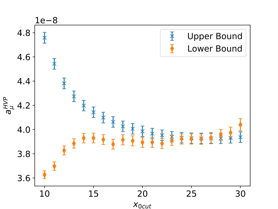 Figure 2
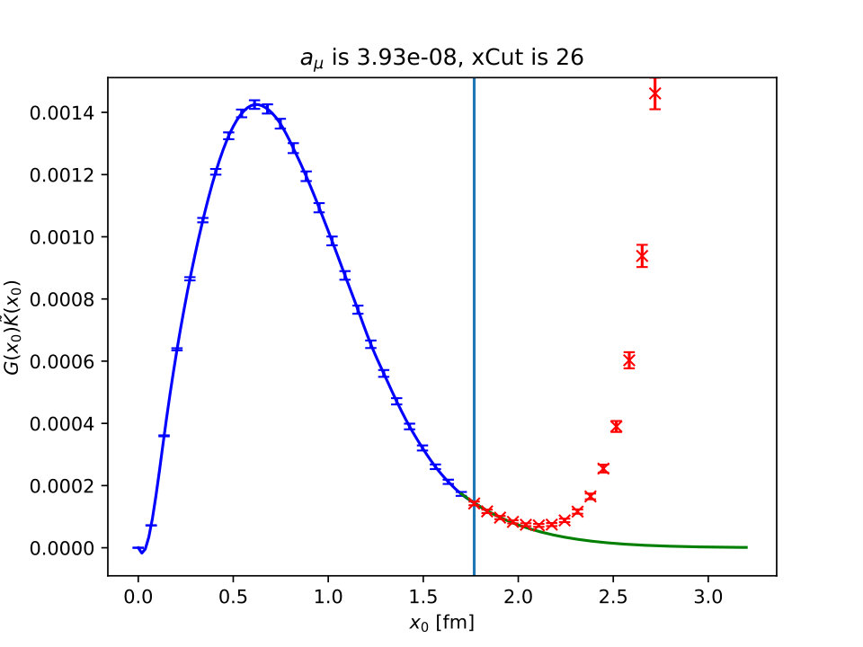 Figure 3
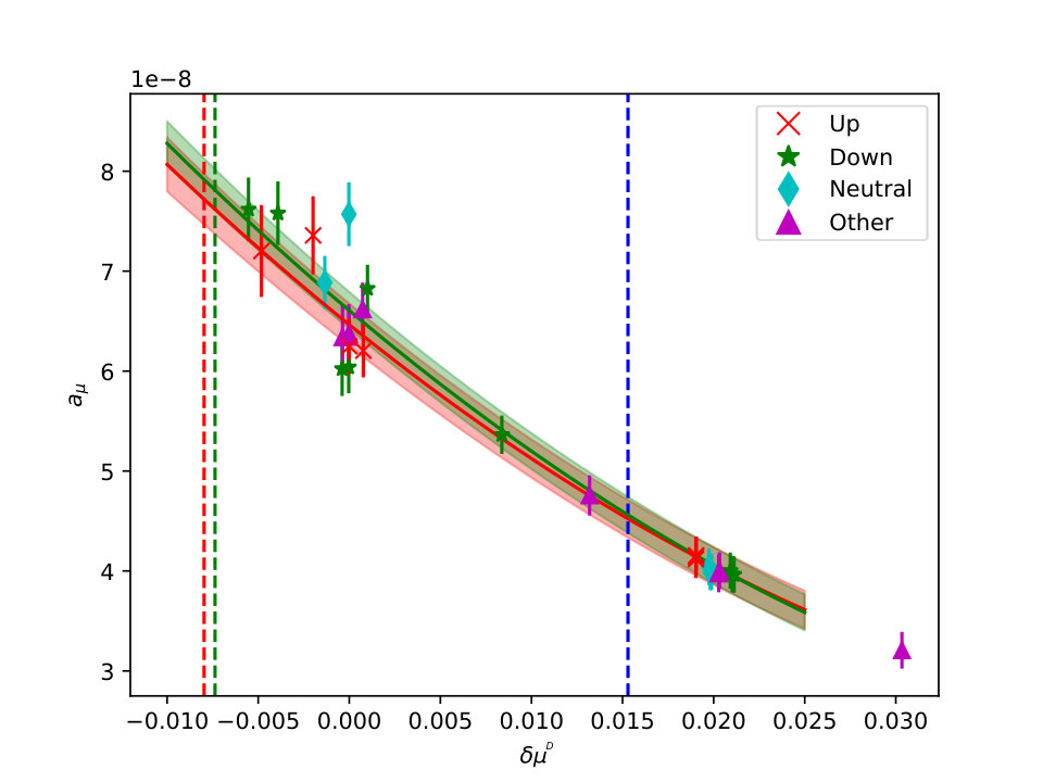 Figure 4
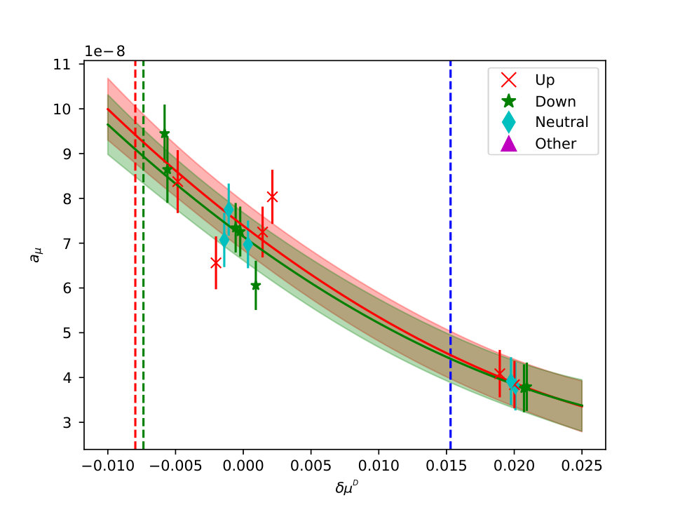 Figure 5
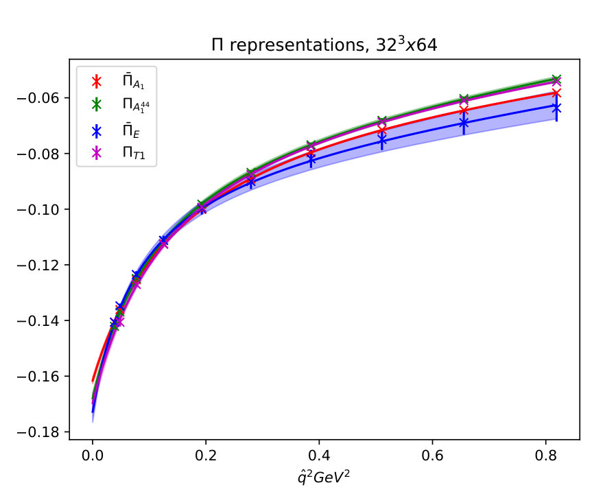 Figure 6
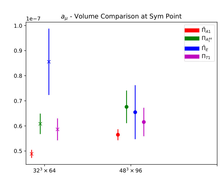 Figure 7
| Ensemble | ||||||||
|---|---|---|---|---|---|---|---|---|
| 1 | 2+1 | 430 | 405 | 405 | 4.4 | 435 | 435 | |
| 2 | 2+1 | 360 | 435 | 435 | 4.0 | 415 | 415 | |
| 3 | 1+1+1 | 290 | 300 | 570 | 3.2 | 320 | 470 | |
| 4 | 2+1 | 430 | 405 | 405 | 6.7 | 435 | 435 | |
| 5 | 2+1 | 360 | 435 | 435 | 5.9 | 420 | 420 |
Peer Reviews
No public reviews on file for this paper yet. If you reviewed it on a platform where reviews are public (OpenReview, ICLR, NeurIPS, ICML), you can paste yours below so the community can read it here.
Videos
No videos yet. Explain this paper in a talk, walkthrough, or lecture? Add one.
Anomalous magnetic moment of the muon with dynamical QCD+QED
A. Westina, R. Horsleyb, W. Kamleha, Y. Nakamurac, H. Perltd, P. E. L. Rakowe, G. Schierholzf A. Schillerd, H. Stübeng, R. D. Younga, ,a
a CSSM, Department of Physics, The University of Adelaide, Adelaide SA 5005, Australia
b School of Physics and Astronomy, University of Edinburgh, Edinburgh EH9 3FD, UK
c RIKEN Advanced Institute for Computational Science, Kobe, Hyogo 650-0047, Japan
d Institut für Theoretische Physik, Universität Leipzig, 04103 Leipzig, Germany
e Theoretical Physics Division, Department of Mathematical Sciences, University of Liverpool, Liverpool L69 3BX, UK
f Deutsches Elektronen-Synchrotron DESY, 22603 Hamburg, Germany
g RRZ, Univeristy of Hamburg, 20146 Hamburg, Germany
E-mail:
CSSM/QCDSF/UKQCD Collaboration
Abstract:
The current discrepancy between experimental and Standard Model determinations of the anomalous magnetic moment of the muon can only be extended to the discovery regime through a reduction of both experimental and theoretical uncertainties. On the theory side, this means a determination of the hadronic vacuum polarisation (HVP) contribution to better than 0.5%, a level of precision that demands the inclusion of QCD + QED effects to properly understand how the behaviour of quarks are modified when their electric charges are turned on. The QCDSF collaboration has generated an ensemble of configurations with dynamical QCD and QED fields with the specific aim of studying flavour breaking effects arising from differences in the quark masses and charges in physical quantities. Here we study these effects in a calculation of HVP around the SU(3) symmetric point. Furthermore, by performing partially-quenched simulations we are able to cover a larger range of quark masses and charges on these configurations and then fit the results to an SU(3) flavour breaking expansion. Subsequently, this allows for an extrapolation to the physical point.
ADP-19-2/T1082
DESY 19-017
LTH 1196
1 Introduction
There currently exists a standard deviation discrepancy between the experimentally measured anomalous magnetic moment of the muon, , and current Standard Model predictions (see e.g. [1]). At present, the experimental [2] uncertainty and the total theoretical uncertainties are of comparable magnitude. The planned Muon Experiment at Fermilab [3] aims to reduce the experimental uncertainty to 140 parts-ber-billion. Thus it is essential to get the theoretical uncertainties down to a comparable precision — this will require the “hadronic vacuum polarisation” (HVP) contributions to be known to better than . Simulations of the QCD-only contribution to HVP have received a surge of interest over the past few years, with results now being quoted at the physical point with errors . At this level of precision, contributions from QED effects are expected to play a role. In this talk, we present preliminary results for the electromagnetic contributions to the hadronic vacuum polarisation tensor — the key ingredient relevant to the QCD contribution to .
2 Accessing
We explore two methods of extracting the HVP contribution to the anomalous magnetic moment from the lattice. First we will take a more traditional approach where we determine the vacuum polarisation from the vacuum polarisation tensor, , as first described in [4, 5]. Secondly we will investigate the time-momentum representation method proposed in [6] to extract a value for .
2.1 Vacuum polarisation tensor
We can calculate from the vacuum polarisation function using
[TABLE]
where is a known kernel function [4], and the polarisation function is determined from the polarisation tensor
[TABLE]
2.2 Time-moment representation
In the time-moment representation (TMR), the vacuum subtracted polarisation function, , is obtained from the spatially summed two-point correlator, ,
[TABLE]
Substituting this into Eq. (1), one finds
[TABLE]
where we employ the analytic form for derived in [7].
3 Simulation details
We follow the flavour-breaking program outlined in [8, 9] originally for QCD, and extended to include electromagnetic interactions in [10, 11]. Starting from the symmetric point , our strategy is to keep the singlet quark mass fixed at its physical value while is varied. This procedure leads to highly constrained polynomials in and , and thus reduces the number of free parameters drastically.
For the partially-quenched, flavour-diagonal () octet (vector) meson masses, with all annihilation channels turned off, a group theoretical analysis incorporating both QCD and QED terms leads to the mass formula to leading order in and second order in
[TABLE]
We have distinguished between sea () and valence (partially-quenched, PQ) quark masses with .
The introduction of quark charges complicates the definition of an SU(3) symmetric point. In [10] we introduced the Dashen scheme which absorbs all electromagnetic effects in the neutral, purely connected pseudoscalar mesons into the definition of the quark mass, which we refer to as the “Dashen mass” . This drastically simplifies the flavour-breaking expansions of the pseudoscalar mesons [10], while the effect on the expansion of the vector mesons as needed here is to replace in Eq. (3) with . A natural definition for the SU(3) symmetric point in this scheme is then one where . This tuning was performed on two volumes in [10].
We employ five ensembles of fully dynamical QCD+QED lattice configuations generated by the QCDSF collaboration, including simulations on two different volumes, , and , with lattice spacing fm, and an exaggerated QED coupling . Our simulation set-up employs the so-called QEDL formulation [12], where the zero mode of the photon field is removed on each time slice for the valence quarks. However, since in this work we only consider electrically neutral hadronic systems, photon zero modes are in any case unlikely to have any effect.
The details of the five ensembles are summarised in Table 1 where we provide the masses of the unitary neutral and charged pseudoscalar mesons. In order to better constrain the coefficients of the flavour-breaking expansions, on each ensemble we employ partially-quenched quark masses corresponding to neutral pseudoscalar meson masses in the range MeV. Quark charges are also partially quenched in that we allow for charges . At our enhanced QED coupling (), the quark charges allow for simulations to be performed with near-physical valence quark charges.
As first observed in [13], we find a clear charge dependence of the vector current renormalisation constant, . This will be discussed in more detail in a forthcoming publication.
4 Results and discussion
4.1 Finite Volume Effects
When working on a finite four-torus with dimensions , the single polarisation function in Eq. (2), as valid for , is replaced by five independent functions corresponding to the five irreducible representations of the finite cubic symmetry group [6, 14]
[TABLE]
These five functions should agree in the infinite volume and continuum limits, hence we are provided with a method for investigating the impact of the finite volume on our results. In left plot of Fig. 1, we display the polarisation functions obtained from the volume close to the SU(3) symmetric point (i.e. ensemble 1 in Table 1). Here we observe a clear discrepancy between the irreducible representations of the vacuum polarisation tensor and indicates the presence of finite volume effects in the simulations.
This behaviour is carried through to after we follow the procedure outlined in Sec. 2.1. This is seen by the scatter of the data points displayed in the right plot of Fig. 1 for the volume. When we repeat the process for the larger volume at the same quark masses (ensemble 2), we observe a pronounced reduction in the scatter of results obtained from the different irreducible representations. This provides us with confidence that results obtained on the larger volume have only a small remnant finite size effect.
4.2 Time Moment
We will now turn our attention to determining from the time moment representation as given in Eq. (5), following the method proposed in [7]. At large times, the 2 point function suffers from a loss of signal into statistical noise and is contaminated by the backwards propagating state. Since Eq. (5) requires to be known to infinite times, this issue is overcome by only using the 2 point function data, up to some value of . After this time, we fit a single exponential with the ground state vector meson mass, , such that
[TABLE]
For the region we use a cubic spline over the lattice data before computing the contribution of this region to the integral in Eq. (5). We choose such that the single exponential ansatz matches the data before the signal is lost to noise, and that it forms a smooth continuous line with the spline of that data at . An example for on ensemble 1 is shown in Fig. 2(a).
We can check our choice of using the recent bounding method [15, 16]. For this we define as
[TABLE]
where we have an upper bound from and a lower bound from . When these two bounds agree, we find the optimal choice for .
In Fig. 2(b) we see that the upper and lower bounds converge at , which matches with when our exponential fit matches on smoothly with in Fig. 2(a).
We note that this procedure can easily be improved by including states beyond the ground state, allowing for smaller values of to be used [15, 16]. This will be pursued in future work.
The above bounding method is then repeated for all partially quenched quarks on all five ensembles in Table 1. We can then calculate on each of our ensembles. These are plotted against the Dashen mass in Fig. 3 for (left) and (right) volumes. Recalling the flavour-breaking expansion for the flavour-diagonal vector mesons given in Eq. (3), then since the SU(3)-flavour properties of are the same, we can apply the same expansion for to extrapolate to the physical masses.
Figure 3 shows our values for plotted against Dashen mass, . Note that for ease of plotting, we have compressed the direction relevant to the variation of with sea quark mass by shifting all points to the physical sea quark masses . The physical values for the valence quark masses are given by the red (up), green (down) and blue (strange) vertical dashed lines. The final value for is obtained by taking the appropriate charge-weighted combination of all three quark flavour contributions at their physical masses. As this work is still preliminary, we refrain from quoting numbers at this stage, however by comparing the results between the volumes it is obvious that there are significant finite volume effects, particularly in the volume. Given the analysis presented in Sec. 4.1, this is not surprising.
Finally, we note that the results from both volumes are described well by the flavour-breaking expansions of Eq. (3) and that our use of partially-quenched valence quarks covering a large range of masses and electric charges allows for contraints to be placed on the various parameters. In particular, we note the small difference in slopes between the red (up quarks with charge ) and green (down/strange quarks with charge ) curves which is a purely electromagnetic effect. In future work we hope to improve the quality of the data and range of ensembles available in order to isolate the contribution from the QED terms.
Acknowledgements
The numerical configuration generation (using the BQCD lattice QCD program [17]) and data analysis (partly using the Chroma software library [18]) was carried out on the IBM BlueGene/Q and HP Tesseract using DIRAC 2 resources (EPCC, Edinburgh, UK), the IBM BlueGene/Q at NIC (Jülich, Germany), the Cray XC40 at HLRN (The North-German Supercomputer Alliance), the NCI National Facility in Canberra, Australia, and the iVEC facilities at the Pawsey Supercomputing Centre. These Australian resources are provided through the National Computational Merit Allocation Scheme and the University of Adelaide Partner Share supported by the Australian Government. This work was supported in part through supercomputing resources provided by the Phoenix HPC service at the University of Adelaide. HP was supported by DFG Grant No. PE 2792/2-1, PELR in part by the STFC under contract ST/G00062X/1 and RDY and JMZ by the Australian Research Council under grants FT120100821, FT100100005, and DP140103067.
The reference list from the paper itself. Each links out to its DOI / PubMed record.
- 1[1] A. Keshavarzi, D. Nomura and T. Teubner, 1802.02995 .
- 2[2] Muon g-2 collaboration, G. W. Bennett et al., Phys. Rev. D 73 (2006) 072003 [ hep-ex/0602035 ]. · doi ↗
- 3[3] Muon g-2 collaboration, A. Chapelain, EPJ Web Conf. 137 (2017) 08001 [ 1701.02807 ]. · doi ↗
- 4[4] T. Blum, Phys. Rev. Lett. 91 (2003) 052001 [ hep-lat/0212018 ]. · doi ↗
- 5[5] QCDSF collaboration, M. Göckeler et al., Nucl. Phys. B 688 (2004) 135 [ hep-lat/0312032 ]. · doi ↗
- 6[6] D. Bernecker and H. B. Meyer, Eur. Phys. J. A 47 (2011) 148 [ 1107.4388 ]. · doi ↗
- 7[7] M. Della Morte et al., JHEP 10 (2017) 020 [ 1705.01775 ]. · doi ↗
- 8[8] W. Bietenholz et al., Phys. Lett. B 690 (2010) 436 [ 1003.1114 ]. · doi ↗