The covering number of the strong measure zero ideal can be above almost everything else
Miguel A. Cardona
Institute of Discrete Mathematics and Geometry, TU Wien, Wiedner Hauptstrasse 8–10/104 A–1040 Wien, Austria.
[email protected]
https://www.researchgate.net/profile/Miguel_Cadona_Montoya
,
Diego A. Mejía
Creative Science Course (Mathematics), Faculty of Science, Shizuoka University, Ohya 836, Suruga-ku, Shizuoka-shi, Japan 422-8529.
[email protected]
http://www.researchgate.com/profile/Diego_Mejia2
and
Ismael E. Rivera-Madrid
Faculty of Engineering, Institución Universitaria Pascual Bravo. Calle 73 No. 73A - 226, Medellín, Colombia.
[email protected]
Abstract.
We show that certain type of tree forcings, including Sacks forcing, increases the covering of the strong measure zero ideal SN. As a consequence, in Sacks model, such covering number is equal to the size of the continuum, which indicates that this covering number is consistently larger than any other classical cardinal invariant of the continuum. Even more, Sacks forcing can be used to force that non(SN)<cov(SN)<cof(SN), which is the first consistency result where more than two cardinal invariants associated with SN are pairwise different. Another consequence is that SN⊆s0 in ZFC where s0 denotes the Marczewski’s ideal.
Key words and phrases:
Strong measure zero sets, cardinal invariants, Sacks model.
2010 Mathematics Subject Classification:
03E17, 03E35, 03E40.
This work was supported by the Austrian Science Fund (FWF) P30666 (first author), the Grant-in-Aid for Early Career Scientists 18K13448, Japan Society for the Promotion of Science (second author), and by the grant no. IN201711, Dirección Operativa de Investigación, Institución Universitaria Pascual Bravo (second and third authors).
1. Introduction
This paper is focused on new consistency results about cardinal invariants associated with the strong measure zero ideal. Recall that the cardinal invariants associated with an ideal I⊆P(X) are
- \mboxadd(I):=min{∣A∣:A⊆I and ⋃A∈/I} the additivity of I;
- \mboxcov(I):=min{∣C∣:C⊆I and ⋃C=X} the covering of I;
- \mboxnon(I):=min{∣Z∣:Z⊆X and Z∈/I} the uniformity of I;
- \mboxcof(I):=min{∣C∣:C⊆I is cofinal in ⟨I,⊆⟩} the cofinality of I.
In this context, we assume that ideals on P(X) contain all the finite subsets of X. Under this assumption, the inequalities indicated in Figure 1 can be proved in ZFC.
A very classical instance of cardinal invariants is Cichoń’s diagram (Figure 2), which is composed by the cardinal invariants associated with the ideal M of meager subsets of R and with the ideal N of Lebesgue-measure subsets of R, by the bounding number b and dominating number d (reviewed in Section 2), and by c=∣R∣=2ℵ0. This diagram is complete in the sense that no other inequalities can be proved (see e.g. [BJ95] for all the details).
Denote by SN the ideal of strong measure zero subsets of R. In relation with the cardinal invariants in Cichoń’s diagram, the following is provable in ZFC:
- (SN1)
\mboxadd(N)≤\mboxadd(SN) (Carlson [Car93]),
2. (SN2)
\mboxcov(N)≤\mboxcov(SN)≤c,
3. (SN3)
\mboxcov(M)≤\mboxnon(SN)≤\mboxnon(N) and \mboxadd(M)=min{b,\mboxnon(SN)} (Miller [Mil81]),
4. (SN4)
\mboxcof(SN)≤2d (see [Osu08]).
On the other hand, the following inequalities are consistent with ZFC:
- (C1)
\mboxcof(M)<\mboxadd(SN) (Goldstern, Judah and Shelah [GJS93]),
2. (C2)
\mboxcov(SN)<\mboxadd(M) (Pawlikowski [Paw90]),
3. (C3)
\mboxnon(SN)<min{b,\mboxcov(N)} (Hechler’s model followed by random model),
4. (C4)
c<\mboxcof(SN) (from CH),
5. (C5)
\mboxcof(SN)<c (Yorioka [Yor02]).
In fact, the forcing model constructed in (C1) satisfies d=ℵ1 and SN=[R]≤ℵ1, so \mboxcof(SN)=c=ℵ2 whenever 2ℵ1=ℵ2 in the ground model. The equality \mboxcof(SN)=c also follows from Borel’s conjecture SN=[R]≤ℵ0, which was proven consistent with ZFC by Laver [Lav76].
The consistency results above show that no other inequality between \mboxadd(SN) and another cardinal in Cichoń’s diagram can be proved, and the same can be said about \mboxnon(SN). However, unsolved problems about \mboxcov(SN) and \mboxcof(SN) still remain.
- (Q1)
Is there a classical cardinal invariant of the continuum (different from c and \mboxcof(SN)) that is an upper bound of \mboxcov(SN)? In particular, is \mboxcov(SN)≤\mboxcof(N)?
2. (Q2)
Is there a classical cardinal invariant of the continuum (different from \mboxcov(N) and \mboxcov(M))111Obvious lower bounds of \mboxcof(SN) are \mboxcov(N) and \mboxcov(M) because of (SN2) and (SN3), respectively. that is a lower bound of \mboxcof(SN)? In particular, is \mboxadd(M)≤\mboxcof(SN)? Is \mboxcof(N)≤\mboxcof(SN)?
In this work, we answer (Q1) in the negative, that is, we show that \mboxcov(SN) is consistently larger than \mboxcof(N) and even larger than any classical cardinal invariant of the continuum (like the almost disjointedness number a, the independence number i and the ultrafilter number u, which are maximal among classical cardinal invariants of the continuum that could be below c). In fact, we show that \mboxcov(SN)=c=ℵ2 in Sacks model (where any classical cardinal invariant of the continuum is ℵ1).
In addition to this, we prove the consistency of \mboxnon(SN)<\mboxcov(SN)<\mboxcof(SN). This is the first consistency result where more than two cardinal invariants associated with SN are pairwise different. For this proof, we use Yorioka’s characterization of \mboxcof(SN) ([Yor02], Theorem 2.6 in this text).
The core of these results are Main Lemma 4.4 and Theorem 4.6, which states that a type of tree forcings (Definition 4.1), and their iterations, increases \mboxcov(SN). In terms of ideals, this implies that SN⊆s0 where s0={X⊆2ω:∀p∈S∃q≤p([q]∩X=∅)} is the Marczewski’s ideal (originally defined in [Mar35]) and S denotes Sacks forcing, so \mboxcov(s0)≤\mboxcov(SN).222Also \mboxnon(SN)≤\mboxnon(s0), but \mboxnon(s0)=c because [2ω]<c⊆s0.
This paper is structured as follows. In Section 2 we review the basic notation and the results this paper is based on. In Section 3 we present preservation results related to the dominating number of κκ for κ regular, this to ensure that \mboxcof(SN) can be manipulated as desired via Yorioka’s characterization theorem. In Section 4 we prove our main results, even more, we show that a type of tree forcings, when iterated, increases \mboxcov(SN). Section 5 is dedicated to discussions and open questions.
2. Preliminaries
We start with a short review of the Tukey order. A relational system is a triplet R=⟨X,Y,⊏⟩ where ⊏ is a relation. Such a relational system has two cardinal invariants associated with it:
- b(R):=min{∣F∣:F⊆X and ¬∃y∈Y∀x∈X(x⊏y)},
- d(R):=min{∣D∣:D⊆Y and ∀x∈X∃y∈D(x⊏y)}.
These cardinals do not exists in general, for example, b(R) does not exists iff d(R)=1; likewise, d(R) does not exists iff b(R)=1.
Let R′:=⟨X′,Y′,⊏′⟩ be another relational system. Say that R is Tukey below R′, denoted by R⪯TR′, if there are maps F:X→X′ and G:Y′→Y such that, for any x∈X and y′∈Y′, if F(x)⊏′y′ then x⊏G(y′). Say that R and R′ are Tukey equivalent, denoted by R≅TR′, if R⪯TR′ and R′⪯TR. Note that R⪯TR′ implies b(R′)≤b(R) and d(R)≤d(R′).
Let κ be an infinite cardinal. For any x,y∈κκ write x≤y for ∀i<κ(x(i)≤y(i)), and define x<y similarly. Define the relation x≤∗y by ∃i0<κ∀i≥i0(x(i)≤y(i)), which we read y dominates x. Say that D⊆κκ is dominating (in κκ) if it is cofinal in ⟨κκ,≤∗⟩, that is, every function in κκ is dominated by some member of D. Denote Dκ:=⟨κκ,κκ,≤∗⟩ and D:=Dω. Define the cardinal invariants bκ:=b(Dκ) and dκ:=d(Dκ).
The classical unbounded and dominating numbers are b:=bω and d:=dω, respectively.
The relational system D1 defined below is relevant in the proof of the main results.
Definition 2.1**.**
Denote by I the set of interval partitions of ω. Define the relational systems D1:=⟨I,I,⊑⟩ and D2:=⟨I,I,⋫⟩ where, for any I,J∈I,
[TABLE]
For each I∈I we define fI:ω→ω and I∗2∈I such that f(n):=minIn and In∗2:=I2n∪I2n+1. For each increasing f∈ωω define the increasing function f∗:ω→ω such that f∗(0)=0 and f∗(n+1)=f(f∗(n)+1), and define If∈I such that Inf:=[f∗(n),f∗(n+1)).
In Blass [Bla10] it is proved that D≅TD1. For completeness, we present the proof and include D2.
Lemma 2.2**.**
D≅TD1≅TD2. Even more, if D⊆ωω is a dominating family of increasing functions, then {If:f∈D} is D1-dominating.
Proof.
To see D1⪯TD note that, for any I∈I and f∈ωω, if f∈ωω is increasing then fI≤∗f implies I⊑If. Indeed, for n large enough, put m:=f∗(n), so f∗(n)=m≤fI(m)<fI(m+1)≤f(m+1)=f∗(n+1), that is, Im⊆Inf.
For D2⪯TD1 note that, for any I,J∈I, I⊑J implies I⋫J∗2. Finally, D⪯TD2 because, for any increasing f∈ωω and I∈I, If⋫I implies f≤∗fI. To show this, notice that If⋫I is equivalent to say that (fI(n),fI(n+1))∩\mboxranf∗=∅ for all but finitely many n. Split into cases: if f=idω, then f∗=idω, so (fI(n),fI(n+1))=∅ for n large enough. Hence, while f(n+1)−f(n)=1, eventually fI(n+1)−fI(n)≥2, which guarantees f≤∗fI.
For the second case, assume f(m0)>m0 for some m0<ω.333Since f is increasing, f≥idω. This implies that f(n)>n for every n≥m0. To guarantee f≤∗fI, it is enough to show that ∣In∩\mboxranf∣≥2 for infinitely many n (recall that In∩\mboxranf=∅ for large enough n). If n∈ω is large enough, then there is some m<ω such that fI(n)<f∗(m)<fI(n+1). On the other hand, since (fI(n+1),fI(n+2))∩\mboxranf∗=∅, f∗(m+1),f(f∗(m))∈In∪In+1. This clearly implies that either In or In+1 intersects \mboxranf in 2 or more points.
∎
Fix b:ω→ω∖{0}.
Denote ∏b:=∏i<ωb(i) and sq<ω(b):=⋃n<ω∏i<nb(i). For each s∈sq<ω(b) define [s]:=[s]b:={x∈∏b:s⊆x}.
The space ∏b, as a topological space endowed with the product topology where each b(i) has the discrete topology, is a compact Polish space with open basis {[s]:s∈sq<ω(b)}. Even more, ∏b is a perfect space whenever b≰∗1.
For combinatorial purposes, we use the notion of strong measure zero in ∏b.
Definition 2.3**.**
For each σ∈(sq<ω(b))ω define htσ∈ωω by htσ(i):=∣σ(i)∣.
Say that X⊆∏b has strong measure zero iff for every f∈ωω there is some σ∈(sq<ω(b))ω with htσ=f such that X⊆⋃i<ω[σ(i)].
Denote SN(∏b):={X⊆∏b:X has strong measure zero}. Likewise, we use the notation SN(R) and SN([0,1]).
When b≰∗1, the map Fb:∏b→[0,1] defined by
[TABLE]
is a continuous onto function, which is one-to-one on the set of sequences in ∏b that are not eventually constant. This map preserves sets between SN(∏b) and SN([0,1]) via images and pre-images, therefore, the value of the cardinal invariants associated with SN do not depend on the space ∏b, neither on R or [0,1].
For σ∈(sq<ω(b))ω define
[TABLE]
The following characterization of SN is quite practical in terms of the sets above.
Lemma 2.4**.**
Let X⊆∏b and let D⊆ωω be a dominating family. Then X∈SN(∏b) iff for every f∈D there is some σ∈(sq<ω(b))ω with htσ=f such that X⊆[σ]∞.
Now we focus on b=2 (as a constant function). Denote pwk:ω→ω the function defined by pwk(i):=ik, and define the relation ≪ on ωω as follows:
[TABLE]
Definition 2.5** (Yorioka [Yor02]).**
For each f∈ωω define
[TABLE]
Any family of the form If with f increasing is called a Yorioka ideal.
Yorioka [Yor02] has proved that If is a σ-ideal when f is increasing. By Lemma 2.4 it is clear that SN=⋂{If:f increasing}. Denote
[TABLE]
It is known that \mboxadd(N)≤minadd≤\mboxadd(M) and \mboxcof(M)≤supcof≤\mboxcof(N) (see [Osu08, CM19]), even more, it is not hard to see that minadd≤\mboxadd(SN). Yorioka’s characterization of \mboxcof(SN) is established as follows.
Theorem 2.6** (Yorioka [Yor02]).**
If minadd=supcof=κ then \mboxcof(SN)=dκ.444In Yorioka’s original result it is further assumed that d=\mboxcov(M)=κ, but this is now known to be redundant.
To finish this section, we review how to increase dκ with κ-Cohen reals. Denote by Fn<κ(I,J) the poset of partial functions from I into J with domain of size <κ, ordered by ⊇.
Lemma 2.7**.**
Let κ and λ be infinite cardinals. If λ>κ<κ then Fn<κ(λ×κ,κ) forces dκ≥λ.
Proof.
Let γ<λ and let {y˙α:α<γ} be a set of Fn<κ(λ×κ,κ)-names of functions in κκ. Since this poset is (κ<κ)+-cc, there is some S∈[λ]<λ such that each y˙α is a Fn<κ(S×κ,κ)-name. A genericity argument guarantees that Fn<κ(κ,κ) adds an unbounded function in κκ over the ground model, so Fn<κ(λ×κ,κ) forces that the κ-Cohen real at ξ∈λ∖S is not dominated by any y˙α.
∎
3. Preservation
In this section, we show a method to preserve dκ large for κ regular. This is a natural generalization of preservation methods by Judah and Shelah [JS90] and Brendle [Bre91]. Our presentation is closer to [CM19, Sect. 4].
Definition 3.1**.**
Let κ be an infinite cardinal. Say that a poset is κκ-good if, for any P-name of a function in κκ, there is some h∈κκ (in the ground model) such that, for any x∈κκ, if x≰∗h then ⊩x≰∗y˙.
Lemma 3.2**.**
Any κκ-good poset forces that dκ≥∣dκV∣.
Proof.
Assume that P is a κκ-good poset and that λ=dκV. Let γ<λ and assume that {y˙α:α<γ} is a set of P-names of functions in κκ. For each α<γ there is some hα∈κκ satisfying goodness for y˙α. Since γ<λ, there is some x∈κκ such that x≰∗hα for any α<γ. Therefore, by goodness, P forces that x≰∗y˙α.
∎
The following couple of lemmas illustrate simple examples of κκ-good posets.
Lemma 3.3** (cf. [Mon17, Lemma 1.46]).**
If κ is regular then any poset of size ≤κ is κκ-good.
Proof.
Let P be a poset of size ≤κ and assume that y˙ is a P-name of a function in κκ. For each p∈P and ξ<κ it is clear that there is some hp(ξ)<κ such that p⊮y˙(ξ)=hp(ξ). Since ∣P∣≤κ<bκ, there is some h∈κκ such that hp≤∗h for any p∈P. It is not hard to see that x≰∗h implies ⊩x≰∗y˙.
∎
Lemma 3.4**.**
If κ is regular then any κ-cc poset is κκ-good.
Proof.
Let P be a κ-cc poset and let y˙ be a P-name of a function in κκ.
Claim 3.5**.**
If α˙ is a P-name of a member of κ then there is some β∈κ such that ⊩α˙<β.
Proof.
Assume the contrary, that is, for any β<κ there is some pβ∈P such that pβ⊩β≤α˙. Since P is κ-cc and κ is regular, there is some q∈P forcing ∣{β<κ:pβ∈G˙}∣=κ, which implies that q⊩κ≤α˙, a contradiction.
∎
For each ξ<κ, apply the claim to find some h(ξ)∈κ such that ⊩y˙(ξ)<h(ξ). It is clear that ⊩y˙<h, therefore, x≰∗h implies ⊩x≰y˙.
∎
Montoya [Mon17, Sect. 1.2.2] defines a canonical forcing Eκ that adds a function in κκ eventually different from the ground model functions in κκ, and she proves that Eκ is κκ-good whenever Eκ forces that κ is measurable.
We finish this section with the following iteration result.
Lemma 3.6**.**
Assume that δ is a limit ordinal and that ⟨Pξ:ξ<δ⟩ is a ⋖-increasing sequence of κκ-good posets. Let P:=\mboxlimdirξ<δPξ. If \mboxcf(δ)>κ and P is \mboxcf(δ)-cc then P is κκ-good.
Proof.
If y˙ is a P-name of a function in κκ, then there is some α<δ such that y˙ is a Pα-name, this because P is \mboxcf(δ)-cc and \mboxcf(δ)>κ. Let h∈κκ be a function obtained from the goodness of Pα applied to y˙. It is clear that x≰∗h implies ⊩Px≰y˙.
∎
4. Tree forcings and the main results
We review the following notation about trees. Say that T⊆ω<ω is a tree if ⟨ ⟩∈T and ∀t∈T∀s⊆t(s∈T). Denote by Lvn(T):=T∩ωω the n-th level of T and, for any s∈T, let Ts:={t∈T:s⊆t or t⊆t}, which is also a tree. Denote by [T]=:{x∈ωω:∀n<ω(x↾n∈T)} the set of infinite branches of T.
Let T⊆ω<ω be a tree. Say that s∈T is a splitting node of T if s⌢⟨i⟩,s⌢⟨j⟩∈T for some i=j. Denote by spl(T) the set of splitting nodes of T. For n<ω, let spln(T) be the set of s∈spl(T) such that there are exactly n-many splitting nodes strictly below s. Given another tree T′⊆ωω, write T′⊆nT when T′⊆T and there is some m<ω such that all the elements of spln(T) have length <m and T′∩ωm=T∩ωm. Note that T′⊆n+1T implies T′⊆nT, and that the relation ⊆n is transitive.
Definition 4.1**.**
Let b:ω→ω∖{0}. We say that a poset T is a b-tree forcing notion if it satisfies the following properties
- (T1)
T is a non-empty set of trees contained in \mboxsq<ω(b).
2. (T2)
If T∈T and s∈T, then there is some splitting note t∈T extending s.
3. (T3)
For T,T′∈T, T′≤T implies T′⊆T.
4. (T4)
If T∈T and s∈T then Ts∈T and Ts≤T.
5. (T5)
If T∈T, n<ω and {St:t∈Lvn(T)}⊆T such that St≤Tt for all t∈Lvn(T), then S:=⋃t∈Lvn(T)St∈T, S≤T and {St:t∈Lvn(T)} is a maximal antichain below S.
6. (T6)
If ⟨Tn:n<ω⟩ is a decreasing sequence in T and Tn+1⊆nTn for al n<ω, then T:=⋂n<ωTn∈T and T≤Tn for all n<ω.
When T is a b-tree forcing for some b we say that T is a bounded-tree forcing notion. Note that (T1) and (T2) imply b≰∗1.
Denote by Tb the poset of all conditions satisfying (T1) and (T2), ordered by ⊆. It is clear that this is a b-tree forcing notion.
Example 4.2**.**
- (1)
Recall Sacks forcing S:=T2 (where 2 represents the constant function with value 2). It is clearly a 2-tree forcing notion.
2. (2)
Let PTb be the poset of conditions T∈Tb such that, whenever s∈spl(T), s⌢⟨i⟩∈T for every i∈b(∣s∣). Judah, Goldstern and Shelah [GJS93] defined this poset and showed that, under CH, there is a CS iteration of such type of posets forcing \mboxadd(SN)=ℵ2 (even more, it shows that SN=[R]≤ℵ1). In particular, these tree forcings are used to prove the consistency result (C1) presented in the introduction.
Lemma 4.3**.**
Any b-tree forcing notion is proper and strongly ωω-bounding.555A poset P is strongly ωω-bounding if for any p∈P and any P-name x˙ of a function from ω into the ground model, there are a function f from ω into the finite sets and some q≤p that forces x˙(n)∈f(n) for any n<ω.
Proof.
The standard argument (see e.g. [GS93]) works thanks to (T6).
∎
The following result is essential to show that b-tree forcings increase \mboxcov(SN). It relies in the notation fixed in Definition 2.1, and in Lemma 2.2.
Main Lemma 4.4**.**
Let T be a b-tree forcing notion and let D⊆ωω be a dominating family of increasing functions. If σf∈(\mboxsq<ω(b))ω with htσf=f∗ for each f∈D then, for any T∈T, there is some S≤T in T and some f∈D such that [σf]∞∩[S]=∅. In particular,
T forces that τ∈/⋂f∈D[σf]∞ where
τ denotes generic real in ∏b added by T.
Proof.
Fix T∈T. Define f:ω→ω such that, for any t∈Lvn(T), there is a splitting node of length <f(n) extending t. By recursion, define g(0)=0 and g(n+1)=f(g(n)), which clearly yields an increasing function g. Set I:=(Ig)∗2, that is, In=[g(2n),g(2(n+1)) for each n<ω. Since D is dominating, by Lemma 2.2 there is some f∈D such that I⊑If∗. For n<ω, choose some kn (if exists) such that Ikn⊆Inf∗. Note that there are only finitely many n<ω for which kn does not exist.
Now we define Tn by recursion on n<ω such that Tnt=Tt for any t∈Lvf∗(n)(Tn). Put T0=T. For the successor step, if kn does not exist then we set Tn+1:=Tn; else, when kn exists, for each t∈Lvg(2kn)(Tn) choose some t′∈Lvg(2kn+1)(T) extending t (recall that f∗(n)≤g(2kn)) such that t′ is incompatible with σn+1f. This is possible because there is a splitting node of length <g(2kn+1) extending t and ∣σn+1f∣=f∗(n+1)≥g(2(kn+1)). Put Tn+1:=⋃t∈Lvf∗(n)(Tn)Tt′. For each t∈Lvf∗(n)(Tn), Tn+1 contains a splitting node of length <f∗(n+1) extending t′. This indicates that ⟨Tn:n<ω⟩ satisfies the conditions of (T6), so S:=⋂n<ωTn∈T and S≤T. Even more, any branch of S is incompatible with σf(k) for all but finitely many k<ω, so [σf]∞∩[S]=∅.
∎
Corollary 4.5**.**
SN⊆s0.
Proof.
Apply Main Lemma 4.4 to T=S.
∎
Now we are ready to prove the main results of this paper.
Theorem 4.6**.**
Assume CH. Then, any CS (countable support) iteration of length ω2 of bounded-tree forcing notions forces \mboxcov(SN)=ℵ2.
Proof.
Assume that ⟨Pα:α≤ω2⟩ results from such iteration and fix any dominating family D of increasing functions in the ground model (by CH, ∣D∣=ℵ1). Let D∗:={f∗:f∈D}, which is also a dominating family. Assume that {X˙ξ:ξ<ω1} is a family of P-names of members of SN(2ω). For each ξ<ω1 and f∈D, there is a P-name σ˙ξf for a function in (2<ω)ω such that P forces htσ˙ξf=f∗ and Xξ⊆[σ˙ξf]∞. Since Pω2 has ℵ2-cc, there is some α<ℵ1 such that σ˙ξf is a Pα-name for each f∈D and ξ<ω1. Let T˙ be a Pα-name of a bounded-tree forcing notion such that Pα+1=Pα∗T˙.
Fix a Pα-generic set G over V. Work in V[G]. Let b:ω→ω be a function such that T:=T˙[G] is a b-tree forcing notion. Thanks to the maps F2 and Fb (see Section 2), since D∗ is still a dominating function in V[G] and ⋂f∈D[σξf]∞∈SN(2ω) for each ξ<ω1, we can find some ρξf∈(\mboxsq<ω(b))ω with htρξf=f∗ for each f∈D and ξ<ω1 such that Fb−1F2′′⋂f∈D[σξf]∞⊆[ρξf]∞. By Main Lemma 4.4, T forces τα∈/⋂f∈D[ρξf]∞ for each ξ<ω1 (here, τα∈∏b is the generic real added by T), so F2−1(Fb(τα))∈/⋂f∈D[σξf]∞ (since τα is a generic real, it can be shown by a density argument that Fb(τα) has a unique pre-image under F2).
Therefore, Pω2 forces that F2−1(Fb(τα))∈/⋃ξ<ω1Xξ.
∎
Theorem 4.7**.**
Assume CH and that λ is an infinite cardinal such that λℵ1=λ. Then, there is a proper ωω-bounding poset with ℵ2-cc forcing \mboxcof(N)=a=u=i=ℵ1, \mboxcov(SN)=ℵ2 and \mboxcof(SN)=λ. In particular, it is consistent with ZFC that \mboxnon(SN)<\mboxcov(SN)<\mboxcof(SN).
Proof.
We show that Fn<ω1(λ×ω1,ω1) followed by the CS iteration of S of length ℵ2 is the desired poset. By CH, Fn<ω1(λ×ω1,ω1) has ℵ2-cc, and it is clear that it is <ω1-closed, so it is proper and preserves cofinalities (and it is obviously ωω-bounding since it does not add new reals). Even more, in the Fn<ω1(λ×ω1,ω1)-forcing extension, CH still holds, 2ℵ1=λ and, by Lemma 2.7, dω1=λ.
Now work in the Fn<ω1(λ×ω1,ω1)-extension. Let Q=⟨Pα,S:α<ω2⟩ be the CS iteration of Sacks forcing of length ω2. It is clear that Q forces \mboxcof(N)=a=u=i=ℵ1 and, by Theorem 4.6, it forces \mboxcov(SN)=c=ℵ2. In addition, since supcof≤\mboxcof(SN), by Theorem 2.6, Q forces that \mboxcof(SN)=dω1.
It remains to show that Q forces dω1=λ. Since Q has ℵ2-cc and size ℵ2, it forces 2ℵ1=λ. On the other hand, for each α<ω2, ∣Pα∣=ℵ1, so Pα is ω1ω1-good by Lemma 3.3. Hence, by Lemma 3.6, Q is ω1ω1-good and, by Lemma 3.2, Q forces λ≤dω1.
∎
Remark 4.8**.**
In the proof above it can be shown in addition that the first ω2-many ω1-Cohen reals form an unbounded family of ω1ω1 even after the iteration of Sacks forcing. Hence, the final model satisfies bω1=ℵ2.
Remark 4.9**.**
Judah, Miller and Shelah [JMS92] have proved that, in Sacks model, \mboxadd(s0)=ℵ1 and \mboxcov(s0)=c. So Corollary 4.5 also implies that \mboxcov(SN)=c in this model.
5. Discussions
Main Lemma 4.4 can also be proved for Silver-like type of posets, or more generally, for lim-sup creature type forcing notions obtained by finitary creating pairs as in [RS99]. Therefore, these type of posets can be included as iterands in Theorem 4.6. Moreover, it can be concluded that SN is contained in the Marczewski-type ideal corresponding to Silver forcing.
Bartoszyński and Shelah [BS02, Thm. 3.3] proved that \mboxnon(SN) can be increased by CS products of Silver-like posets. In fact, the same argument applies to CS products of posets of the form PTb with b diverging to infinity. Concretely, assuming CH, if κℵ0=κ, I is a set of size κ and {bi:i∈I}⊆ωω is a family of functions diverging to infinity, then the CS product of PTbi with i∈I forces d=ℵ1 (it is ωω-bounding) and \mboxnon(SN)=c=κ.
A very natural question that comes from our main result is whether a version of Theorem 4.6 for CS products can be proved. By methods like in [GS93, KM] it can be shown that any CS product of bounded-tree forcing notions remains proper and strongly ωω-bounding. However, it is not obvious how the proof of Main Lemma 4.4 can be translated to show that such a CS product increases \mboxcov(SN). This would generalize the consistency result of Theorem 4.6 in the sense that \mboxcov(SN) could be forced larger than ℵ2.
By well known methods and results from [Yor02], the following open problem is the only one remaining to settle that the diagram of inequalities in Figure 3 is complete.
Question 5.1**.**
Is it consistent with ZFC that \mboxadd(SN)<min{\mboxcov(SN),\mboxnon(SN)}?
This work provides the first example where 3 cardinals associated with SN can be pairwise different. To go one step further, we propose the following problem.
Question 5.2**.**
Is it consistent with ZFC that the four cardinal invariants associated with SN are pairwise different?
The following idea may be useful to answer the question above.
Quite recently, the first and third authors with Brendle [BCM] constructed a ccc poset forcing
[TABLE]
In the same model, \mboxcov(SN)=\mboxcov(N)<\mboxnon(SN)=\mboxnon(N) by (S3) and because this model is obtained by a FS iteration of length with cofinality μ (where μ is the desired value for \mboxnon(M)), and it is well known that such cofinality becomes an upper bound of \mboxcov(SN) (see e.g. [BJ95, Lemma 8.2.6]). However, tools to deal with \mboxadd(SN) and \mboxcof(SN) in this situation are still unknown.
It would also be very useful to have a stronger characterization of \mboxcof(SN). So far, Theorem 2.6 is restricted to minadd=supcof, which implies \mboxadd(SN)=\mboxnon(SN), so another characterization that allows \mboxadd(SN)<\mboxnon(SN) would lead to methods to solve Question 5.2.

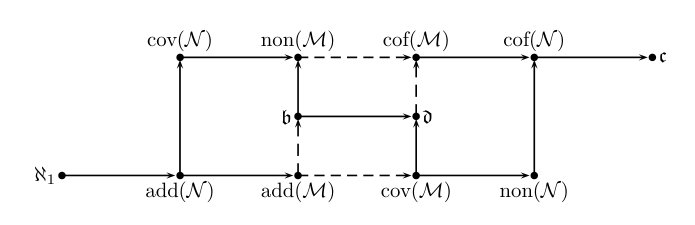 Figure 1
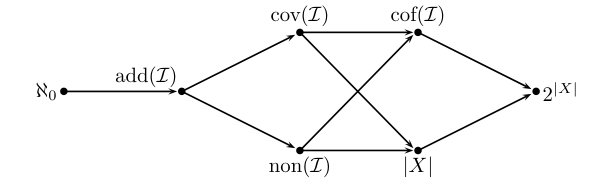 Figure 2
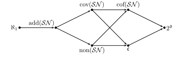 Figure 3