What is the dimension of your binary data?
Nikolaj Tatti, Taneli Mielikainen, Aristides Gionis, Heikki Mannila

TL;DR
This paper introduces a normalized fractal dimension to measure the effective complexity of binary datasets, capturing dependency structures more robustly than traditional methods like PCA.
Contribution
It adapts the concept of fractal dimension for binary data and proposes a normalized version that quantifies variable dependencies more effectively.
Findings
Normalized fractal dimension correlates with data dependency structures.
It provides a more interpretable measure than traditional fractal dimension.
Differences observed between dataset and subgroup dimensions.
Abstract
Many 0/1 datasets have a very large number of variables; on the other hand, they are sparse and the dependency structure of the variables is simpler than the number of variables would suggest. Defining the effective dimensionality of such a dataset is a nontrivial problem. We consider the problem of defining a robust measure of dimension for 0/1 datasets, and show that the basic idea of fractal dimension can be adapted for binary data. However, as such the fractal dimension is difficult to interpret. Hence we introduce the concept of normalized fractal dimension. For a dataset , its normalized fractal dimension is the number of columns in a dataset with independent columns and having the same (unnormalized) fractal dimension as . The normalized fractal dimension measures the degree of dependency structure of the data. We study the properties of the normalized fractal…
Click any figure to enlarge with its caption.
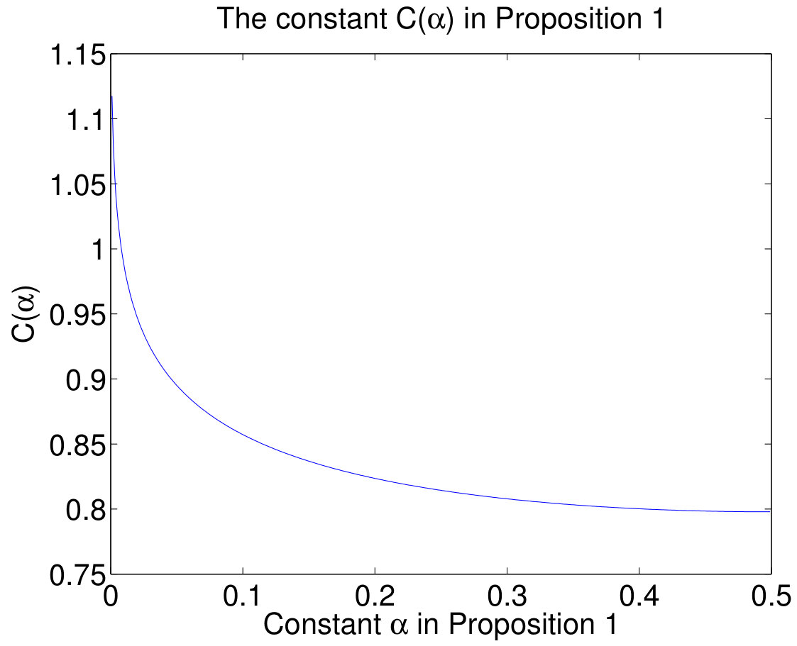 Figure 1
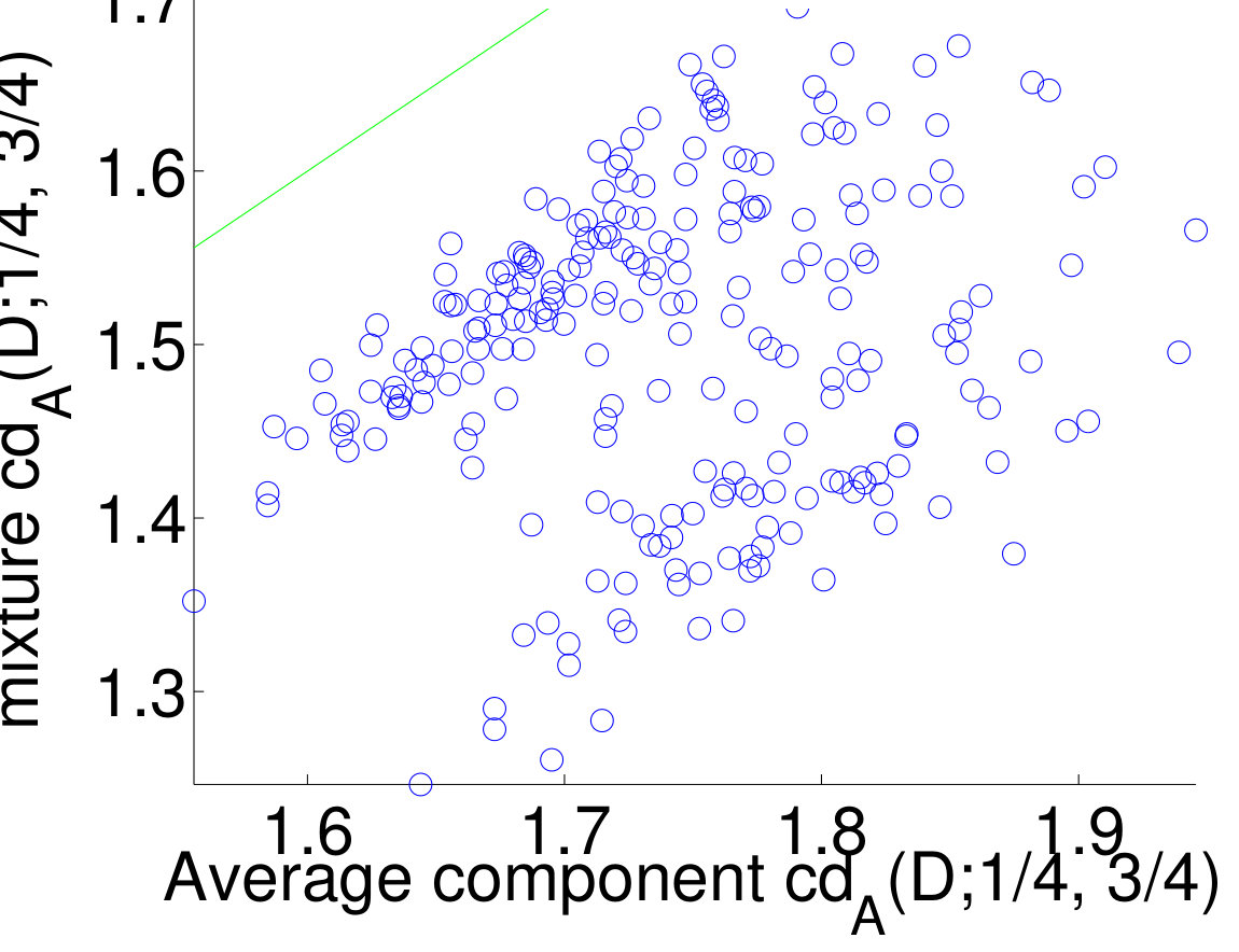 Figure 2
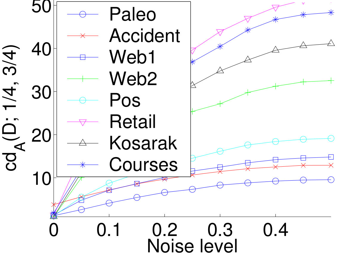 Figure 3
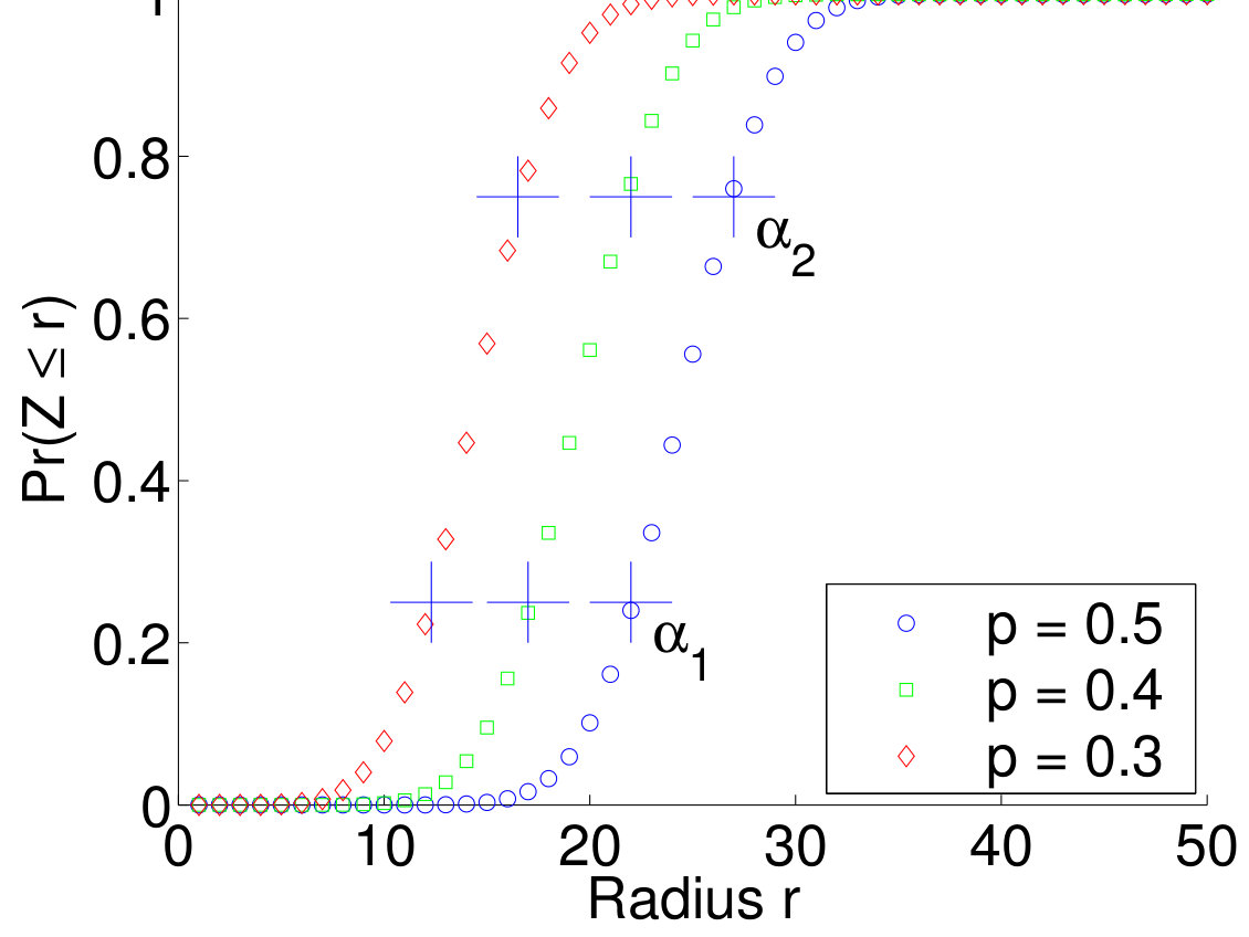 Figure 4
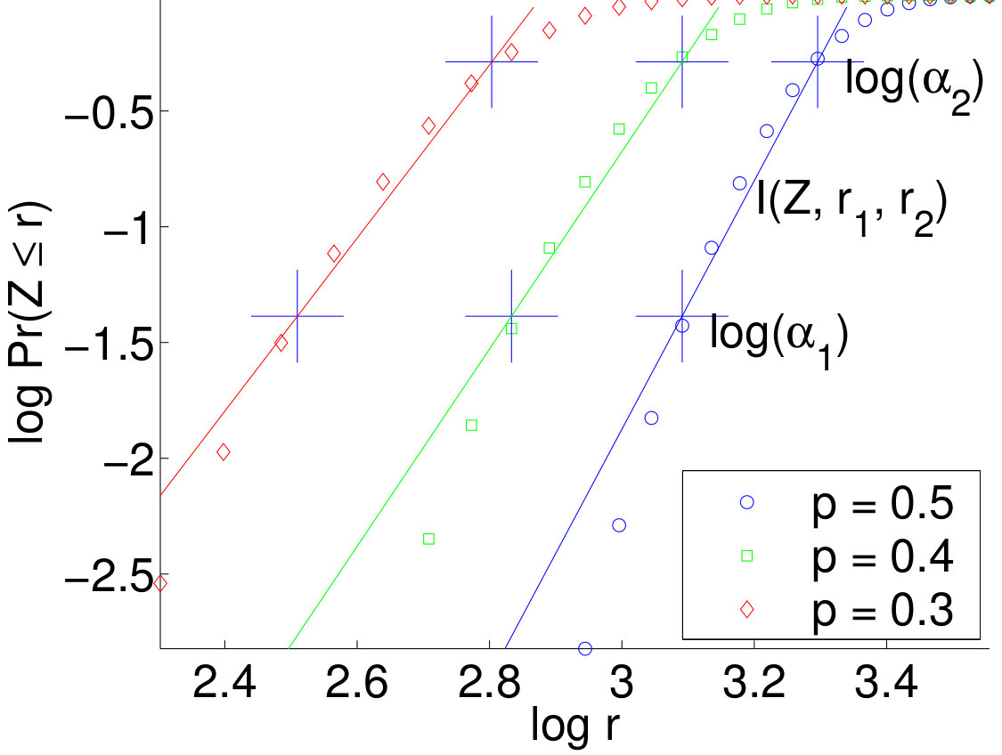 Figure 5
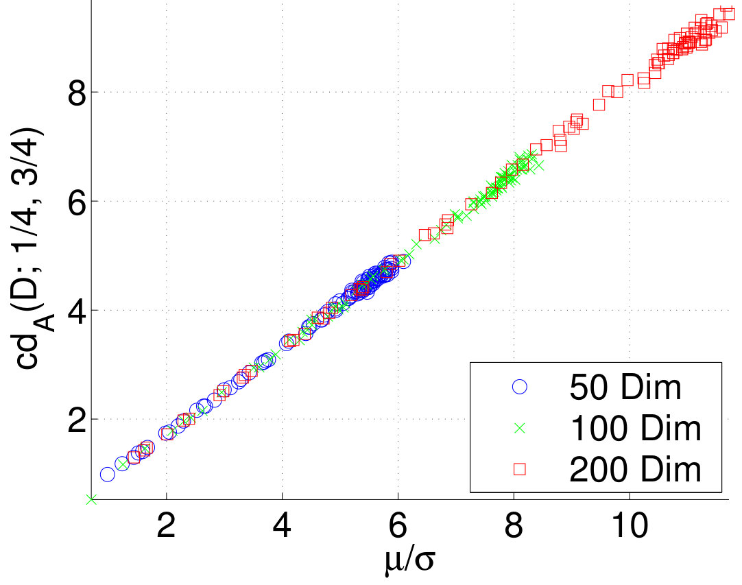 Figure 6
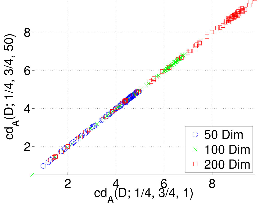 Figure 7
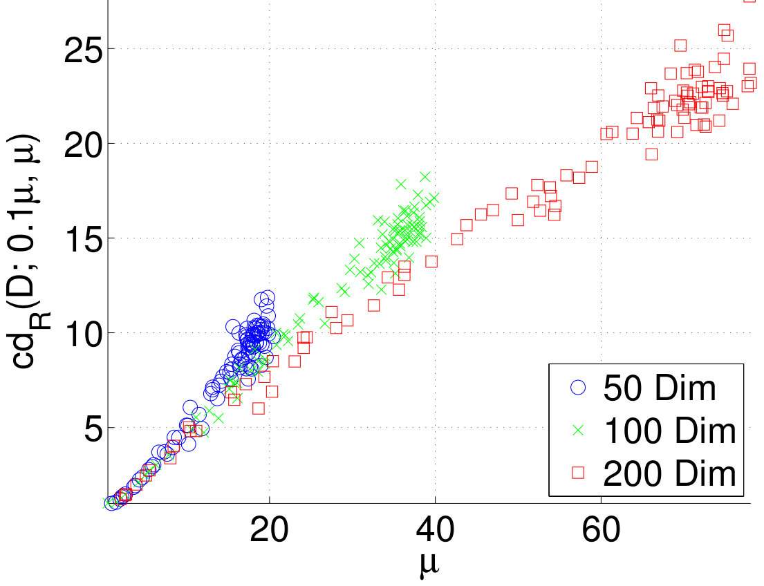 Figure 8
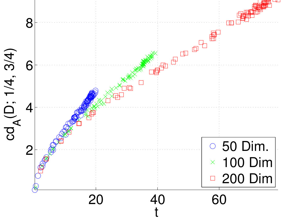 Figure 9
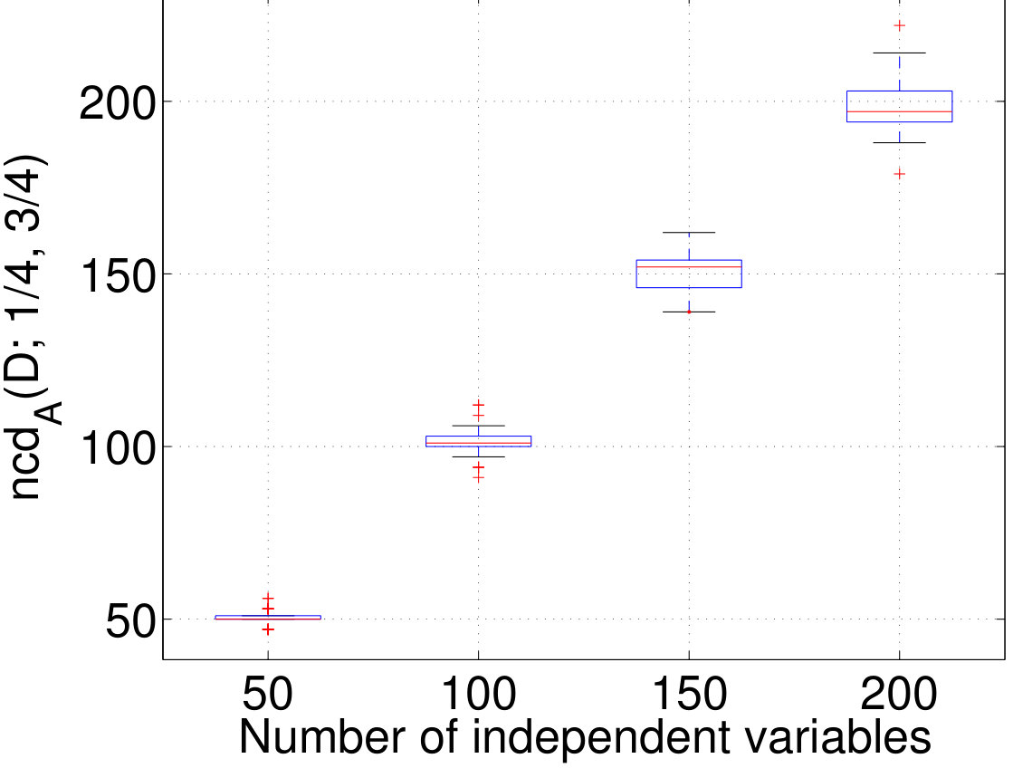 Figure 10
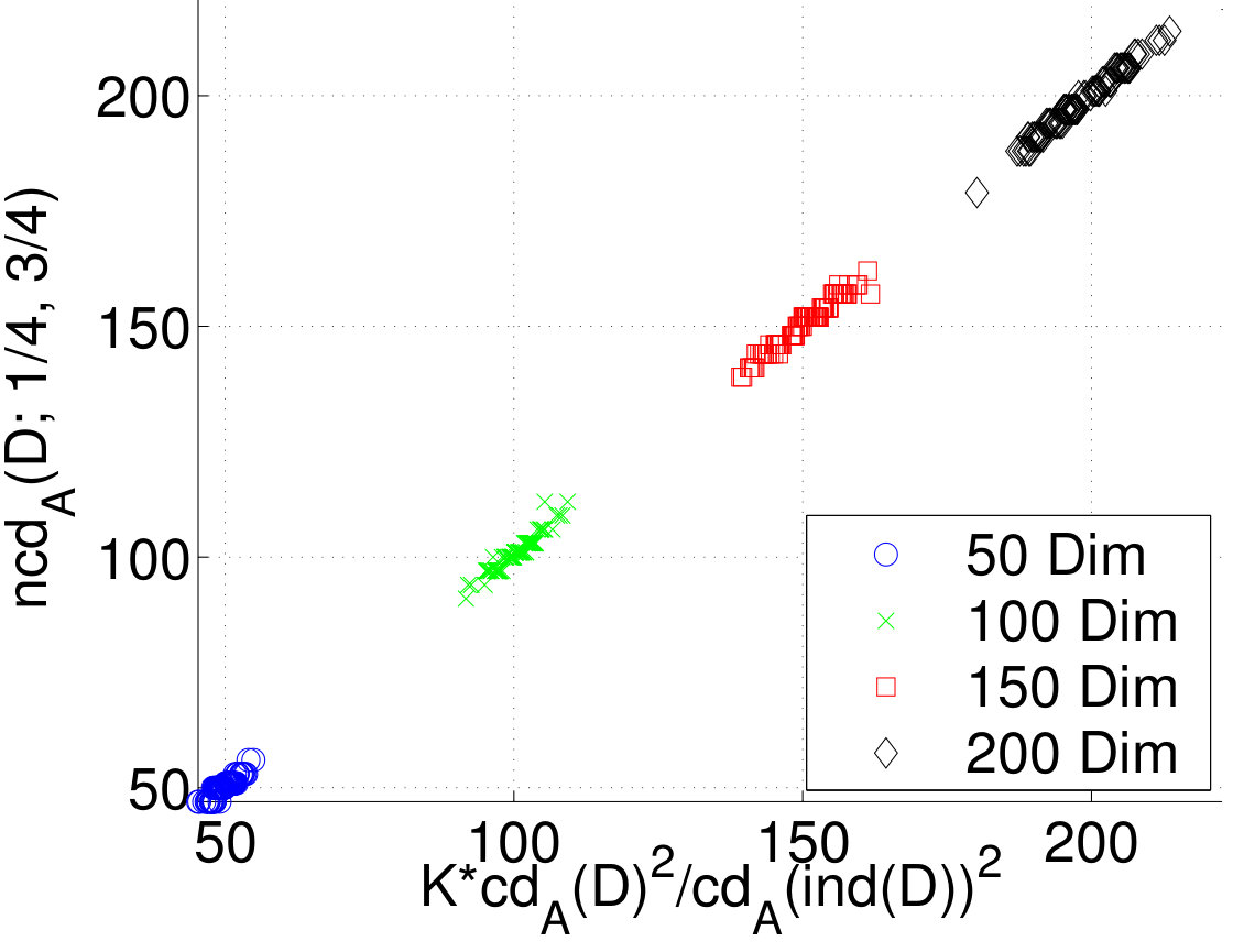 Figure 11
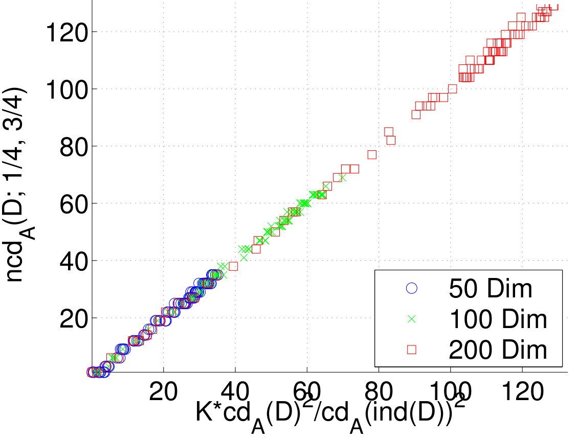 Figure 12
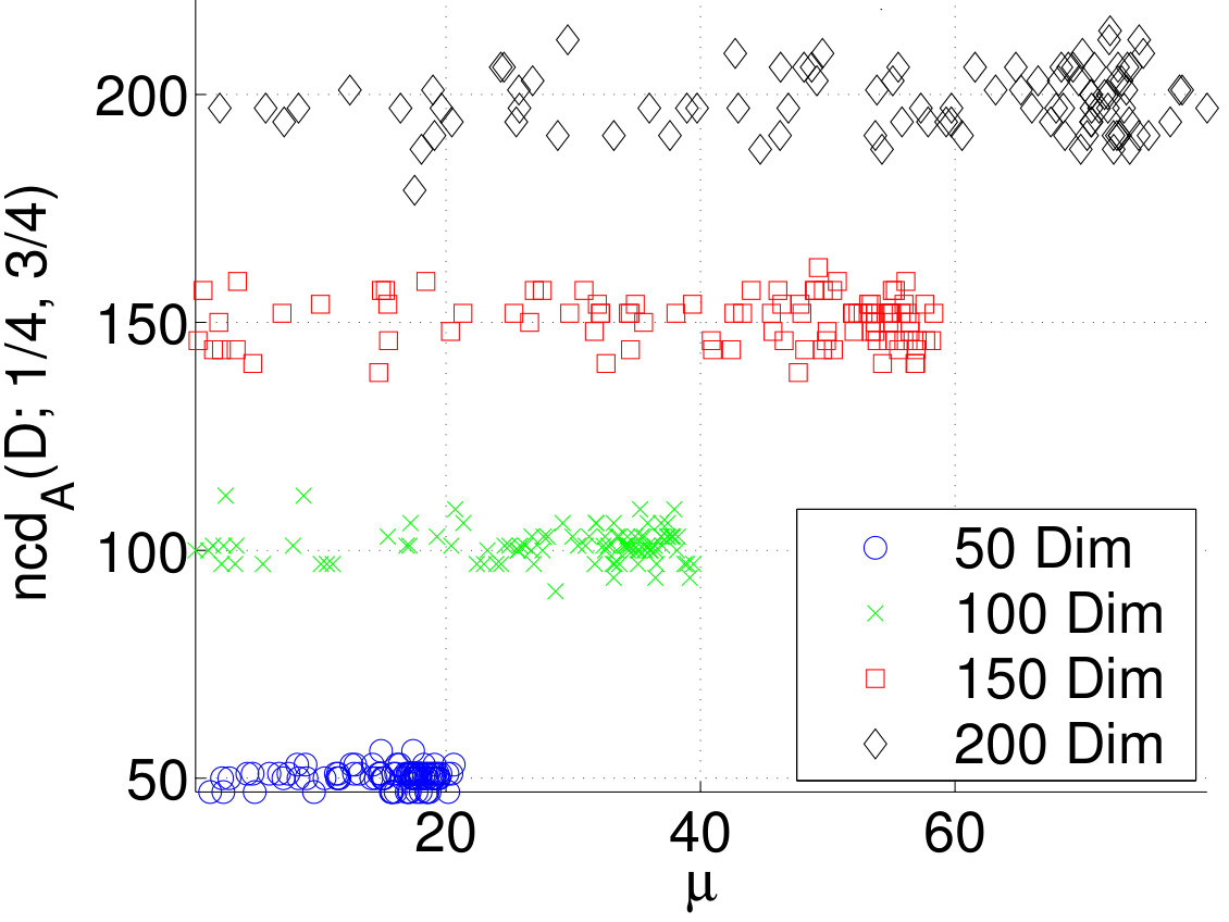 Figure 13
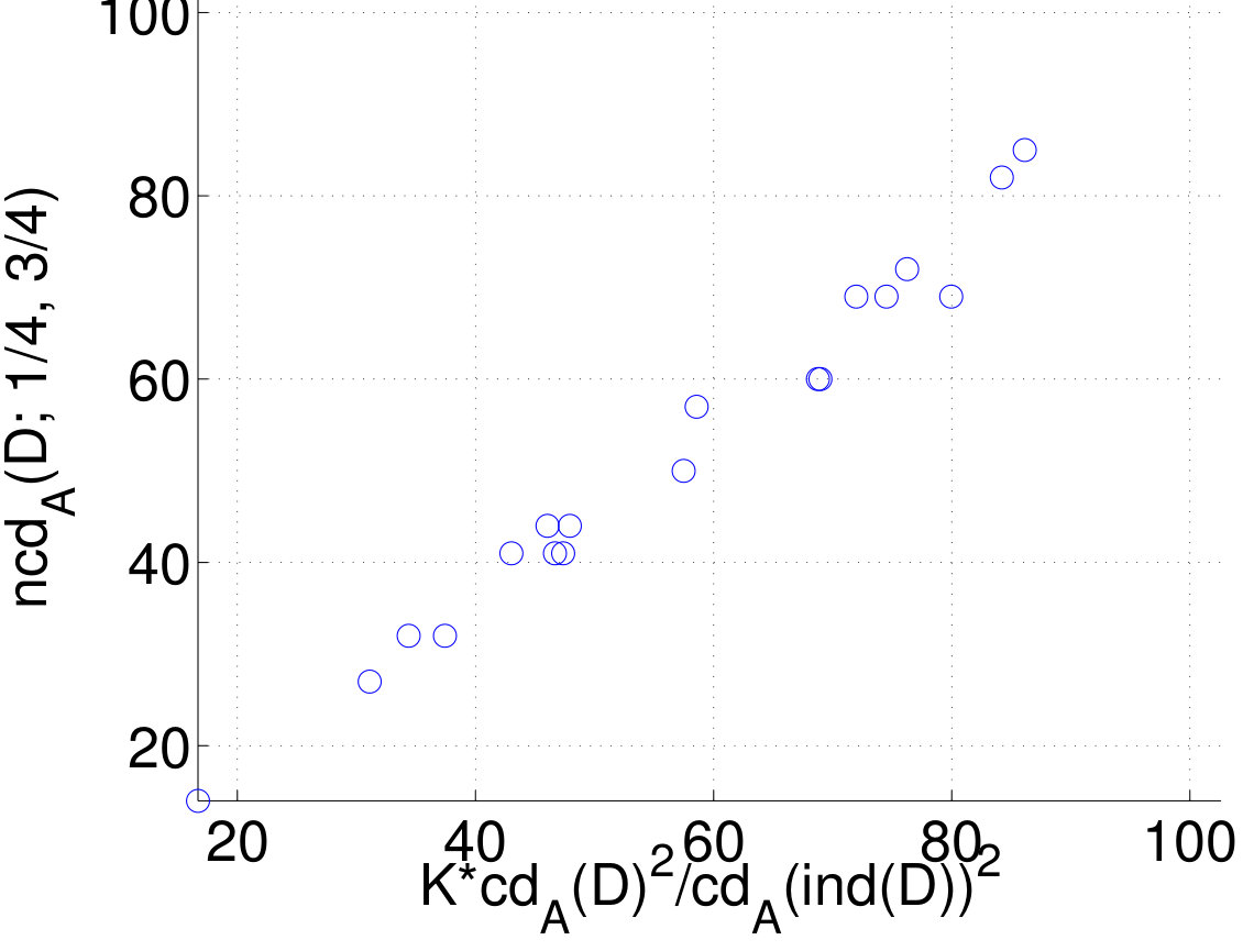 Figure 14
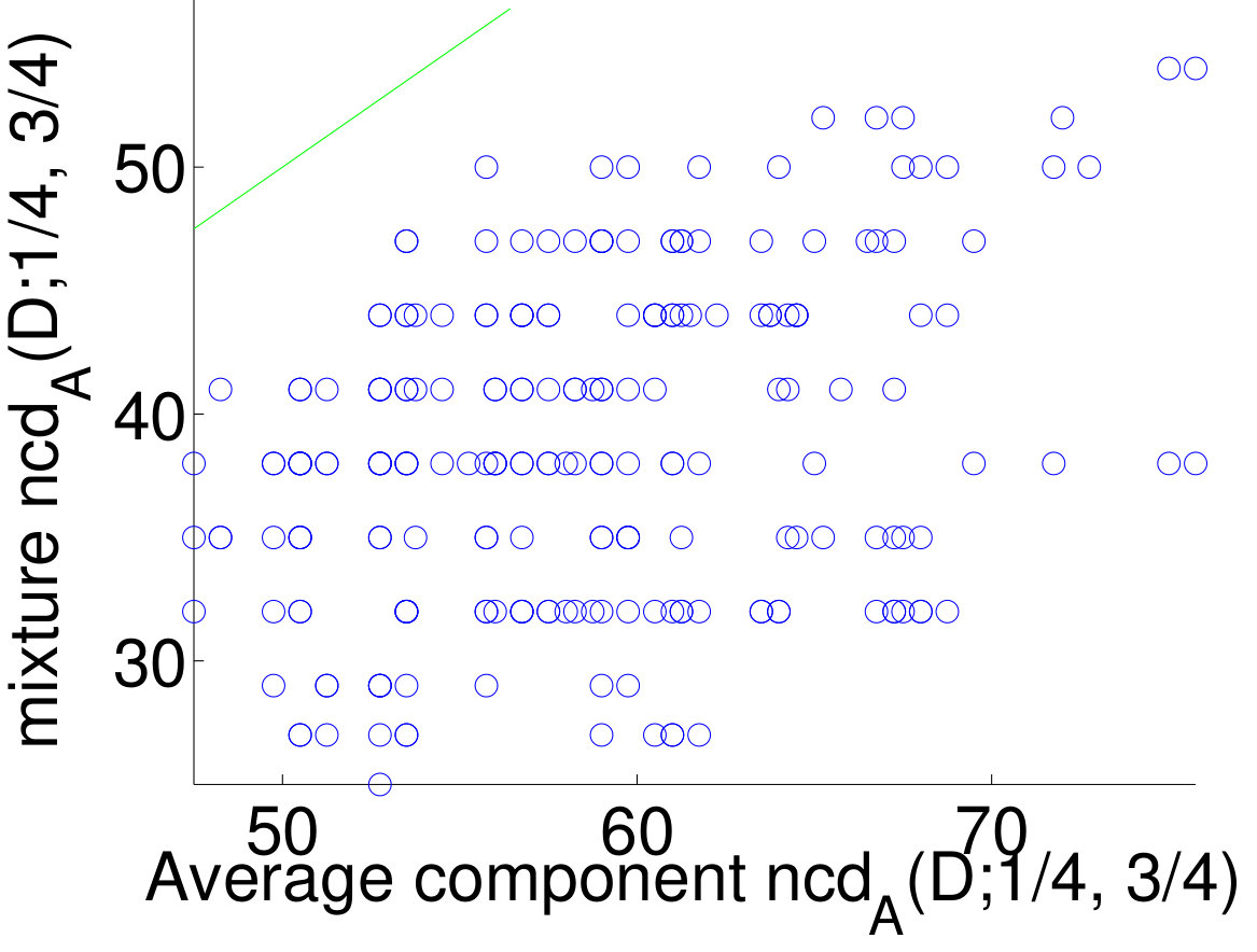 Figure 15
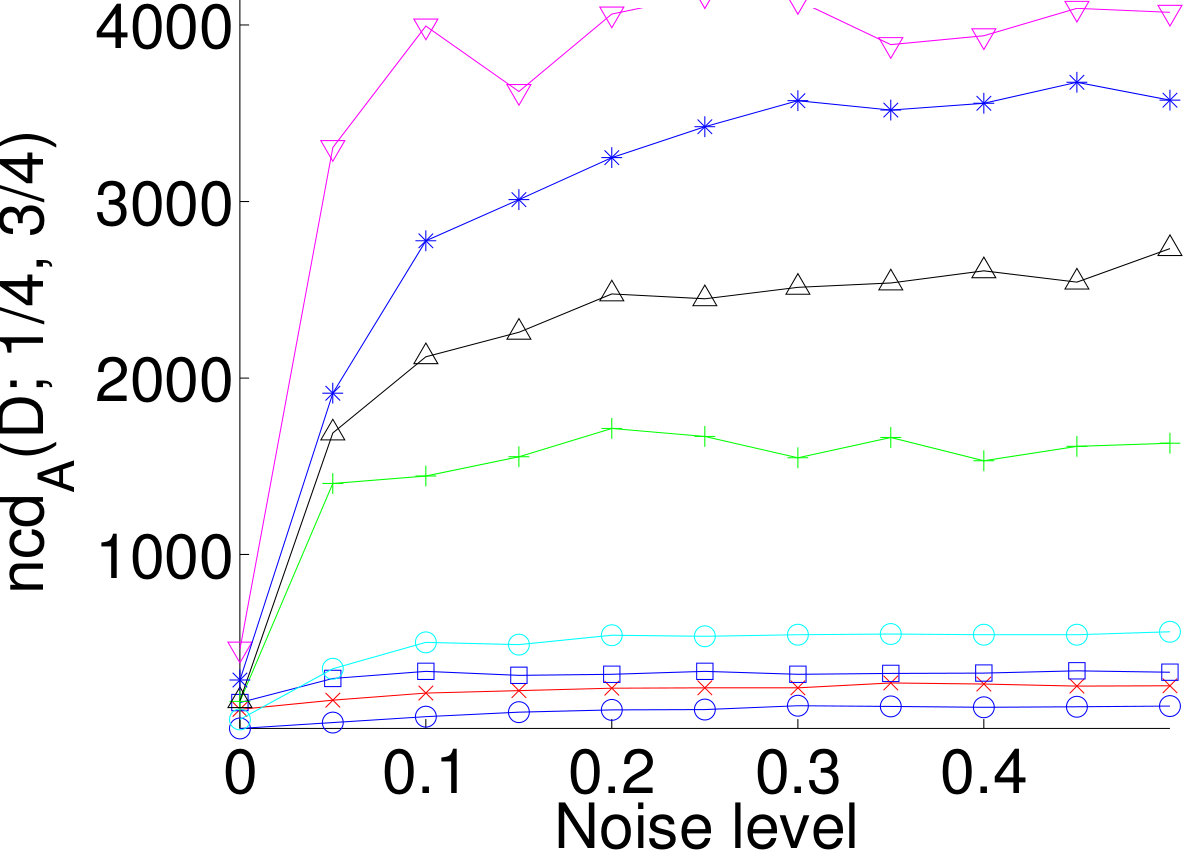 Figure 16
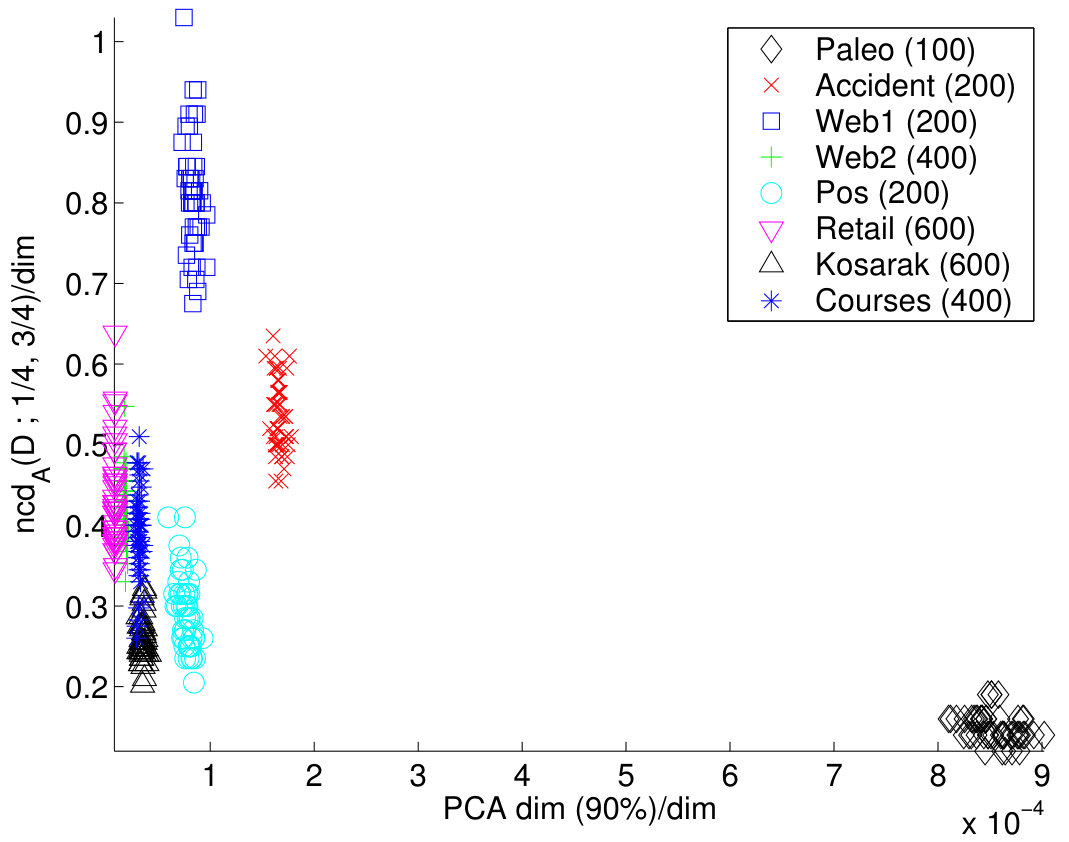 Figure 17
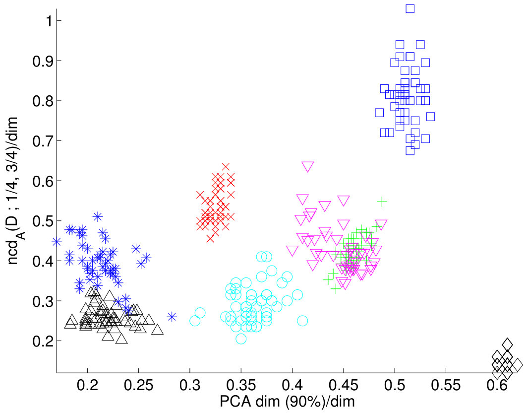 Figure 18
| Data | # of 1s | Dens. | ||
|---|---|---|---|---|
| Accidents | ||||
| Courses | ||||
| Kosarak | ||||
| Paleo | ||||
| POS | ||||
| Retail | ||||
| WebView-1 | ||||
| WebView-2 |
| Data | ||||
|---|---|---|---|---|
| Accidents | ||||
| Courses | ||||
| Kosarak | ||||
| Paleo | ||||
| POS | ||||
| Retail | ||||
| WebView-1 | ||||
| WebView-2 |
| Data | ||||
|---|---|---|---|---|
| Accidents | ||||
| Courses | ||||
| Kosarak | ||||
| Paleo | ||||
| POS | ||||
| Retail | ||||
| WebView-1 | ||||
| WebView-2 |
| Data | # of 1’s | Time | Time/# of 1’s |
|---|---|---|---|
| Accidents | |||
| Courses | |||
| Paleo | |||
| Kosarak | |||
| POS | |||
| Retail | |||
| WebView-1 | |||
| WebView-2 |
| Data | PCA () | PCA Dim. | |
|---|---|---|---|
| Accidents | |||
| Paleo | |||
| POS | |||
| WebView-1 | |||
| WebView-2 |
| vs. | ||
| Data | PCA () | |
| Accident | ||
| Courses | ||
| Kosarak | ||
| Paleo | ||
| POS | ||
| Retail | ||
| WebView-1 | ||
| WebView-2 | ||
| Total | ||
| Total without Paleo | ||
| Data | # of rows | ||
|---|---|---|---|
| Cluster 1 | |||
| Cluster 2 | |||
| Cluster 3 | |||
| Average | – | ||
| Whole data |
Peer Reviews
No public reviews on file for this paper yet. If you reviewed it on a platform where reviews are public (OpenReview, ICLR, NeurIPS, ICML), you can paste yours below so the community can read it here.
Videos
No videos yet. Explain this paper in a talk, walkthrough, or lecture? Add one.
Taxonomy
MethodsPrincipal Components Analysis
What is the dimension of your binary data?
Nikolaj Tatti Taneli Mielikäinen Aristides Gionis Heikki Mannila
HIIT Basic Research Unit, Department of Computer Science
University of Helsinki and Helsinki University of Technology
Abstract
Many 0/1 datasets have a very large number of variables; on the other hand, they are sparse and the dependency structure of the variables is simpler than the number of variables would suggest. Defining the effective dimensionality of such a dataset is a nontrivial problem. We consider the problem of defining a robust measure of dimension for 0/1 datasets, and show that the basic idea of fractal dimension can be adapted for binary data. However, as such the fractal dimension is difficult to interpret. Hence we introduce the concept of normalized fractal dimension. For a dataset , its normalized fractal dimension is the number of columns in a dataset with independent columns and having the same (unnormalized) fractal dimension as . The normalized fractal dimension measures the degree of dependency structure of the data. We study the properties of the normalized fractal dimension and discuss its computation. We give empirical results on the normalized fractal dimension, comparing it against baseline measures such as PCA. We also study the relationship of the dimension of the whole dataset and the dimensions of subgroups formed by clustering. The results indicate interesting differences between and within datasets.
1 Introduction
Many 0/1-datasets occurring in data mining are on one hand complex, as they have a very high number of columns. On the other hand, the datasets can be simple, as they might be very sparse or have lots of structure. In this paper we consider the problem of defining a notion of effective dimension for a binary dataset. We study ways of defining a concept of dimension that would somehow capture the complexity or simplicity of the dataset. Such a notion of effective dimension can be used as a general score describing the complexity or simplicity of the dataset; Some potential applications of the intrinsic dimensionality of a dataset include model selection problems in data analysis; it can also be used in speeding up certain computations (see, e.g., [9]).
For continuous data there are many ways of defining the dimension of a dataset. One approach is to use decomposition methods such as SVD, PCA, or NMF (nonnegative matrix factorization) [14, 19] and to count how many components are needed to express, say, of the variance in the data. This number of components can be viewed as the number of effective dimensions in the data.
In the aforementioned methods it is assumed that the dataset is embedded into a higher-dimensional space by some (smooth) mapping. The other main approach is to use a different concept, that of fractal dimensions [3, 9, 15, 23]. Very roughly, the concept of fractal dimension is based on the idea of counting the number of observations in a ball of radius and looking what the rate of growth of the number is as a function of . If the number grows as , then the dimensionality of the data can be considered to be . Note that this approach does not provide any mapping that can be used for the dimension reduction. Such mapping does not even make sense because the dimension can be non-integral.
Applying these approaches to binary data is not easy. Many of the component methods, such as PCA and SVD are strongly based on the assumption that the data are real-valued. NMF looks for a matrix decomposition with nonnegative entries and hence is somewhat better suited for binary data. However, the factor matrices may have continuous values, which makes them difficult to interpret. The component techniques aimed at discrete data (such as multinomial PCA [6] or latent Dirichlet allocation (LDA) [4]) are possible alternatives, but interpreting the results is hard.
In this paper we explore the notion of effective dimension for binary datasets by using the basic ideas from fractal dimensions. Essentially, we consider the distribution of the pairwise distances between random points in the dataset. Denoting by this random variable, we study the ratio of and , for different values of the , and fit a straight line to this; the slope of the line is the correlation dimension of the dataset.
Interpreting the correlation dimension of discrete data turns out to be quite difficult too, because the values of the correlation dimension tend to very small. To relieve this problem, we normalize them by considering what would be the number of variables in a dataset with the same correlation dimension but with independent columns. This normalized correlation dimension is our main concept.
We study the behavior of the correlation dimension and the normalized correlation dimension, both theoretically and empirically. We give approximations for correlation dimension, in the case of independent variables, showing that it decreases when the data becomes more sparse. We also give theoretical evidence indicating that positive correlations between the variables lead to smaller correlation dimensions.
Our empirical results for generated data show that the normalized correlation dimension of a dataset with independent variables is very close to , irrespective of the sparsity of the attributes. We demonstrate that adding positive correlation decreases the dimension. For real datasets, we show that different datasets have quite different normalized correlation dimensions, and that the ratio of the number of variables to the normalized correlation dimension varies a lot. This indicates that the amount of structure in the datasets is highly variable. We also compare the normalized correlation dimension against the number of PCA components needed to explain of the variance in the data, showing interesting differences among the datasets.
The rest of this paper is organized as follows. In Section 2 we define the correlation dimension for binary datasets. we analyze the correlation dimension in Section 3. The correlation dimension produces too small values and hence in Section 4 we provide means for scaling the dimension. In Section 5 we represent our tests with real world datasets. In Section 6 we review the related literature, and Section 7 is a short conclusion.
2 Correlation Dimension
There are several possible definitions of the fractal dimension of a subset of the Euclidean space; see, e.g., [3, 23] for a survey; the Rényi dimensions [23] form a fairly general family. The standard definitions of the fractal dimension are not directly applicable in the discrete case, but they can be modified to fit in.
The basic idea in the fractal dimensions is to study the distance between two random data points.
We focus on the correlation dimension. Consider a 0/1 dataset with variables. Denote by the random variable whose value is the distance between two randomly chosen points from ; thus . Informally, the correlation dimension is the slope of the line fitted in the log-log plot of .
The more formal definition is more complex because the non-continuity of causes misbehavior in our later definitions. To remedy these problems we first define function to be . We extend this function to real numbers by linear interpolation. Thus is a continuous function being equal to when is an integer.
Let . Then the different radii and the function for a given dataset determine the point set
[TABLE]
We usually omit the parameter for the sake of brevity.
For example, assume that for some , that is, the number of pairs of points within distance grows as . Then is a straight line and the correlation dimension is equal to .
Definition 1**.**
The correlation dimension for a binary dataset and radii and is the slope of the least-squares linear approximation .
Assume that we are given and such that . We define to be , where the radii are set to be . The reason for truncating is to avoid some misbehavior occurring with extremely sparse datasets.
That is, is the set of points containing the logarithm of the radius and the logarithm of the fraction of pairs of points from that have distance less than or equal to . The correlation dimension is the slope of the line that fits these points best. The difference between and is that is defined by using the absolute bounds and for the radius , whereas uses the parameters and to specify the sizes of the tail of the distribution. For instance, is the correlation dimension obtained by first computing the values and such that one quarter of the pairs of points have distance below , and one quarter of the pairs have distance above . The dimension is then obtained by computing points with , and by fitting a line to these points, in the least-squares sense.
How can we compute the correlation dimension of a binary dataset ? The probability can be computed
[TABLE]
where is the indicator function having value if , and value [math] otherwise. Computing the values for all can thus be done trivially in time , where is the number of points in and is the number of variables. A sparse matrix representation yields to a running time of , where is the total number of 1’s in the data: If point has 1’s, then , and computing the all pairwise distances takes time
[TABLE]
If the number of points in a dataset is so large that quadratic computation time in the number of points is too slow, we can take a random subset from and estimate the probability by
[TABLE]
or by
[TABLE]
3 Properties of binary correlation dimension
In this section we analyze the properties of the correlation dimension for binary datasets. We show the following results under some simplifying assumptions. First, we prove that if the original data has independent columns, then the correlation dimension grows as the probabilities of the individual variables get closer to . Second, we show that in the independent case grows as , where is the number of attributes (columns) in the dataset. Third, we prove that if the variables are not independent, then the correlation dimension is smaller than for a dataset with the same margins but independent variables.
The analysis is not easy, and we need to make some simplifying assumptions. One complication is caused by the fact that the definition of involves computing the slope of a set of points. However, note that contains only two points, and hence we have
[TABLE]
Similarly, in the case of we have and such that , and hence
[TABLE]
Throughout this section we will assume that the parameter in is equal to .
Proposition 2**.**
Assume that the dataset has independent variables, and that the probability of the variable being 1 is for each , and let . Assuming that is large enough, we have
[TABLE]
where is a constant depending only on . In particular, if all probabilities are equal to , then for we have
[TABLE]
The proposition indicates that the correlation dimension is maximized for variables as close to as possible.
Corollary 3**.**
Assume the dataset has independent columns. The correlation dimension is maximized if the variables have frequency .
The proposition also tells that for a dataset with independent identically distributed columns, the dimension grows as a square root of the number of columns.
Proof of Proposition 2.
Recall that
[TABLE]
where and are such that and . The numerator is . Assume that is large enough that we can estimate by .
We next study the denominator . We have to analyze the distribution of the random variable , the distance between two randomly chosen points from . For simplicity, we denote by in the sequel. Let be the indicator variable having value 1 if two randomly chosen elements from disagree in variable ; then .
Denote by the probability that two randomly chosen points from differ in coordinate . If is the probability that variable in has value , then , and it is easy to see that .
As , the variable has a binomial distribution. For simplicity we use the normal approximation: is distributed as , where and . If is large enough, this approximation is accurate.
By the symmetry of the normal distribution there is a constant such that and . Actually, is the inverse of the cumulative distribution function of the normal distribution with parameters 0 and 1, i.e., The denominator is
[TABLE]
Dropping all but the two first terms and using the series for logarithm we obtain that the numerate is
[TABLE]
By setting
[TABLE]
we have the desired result. ∎
If , then the constant in Proposition 2 is about .
The correlation dimension has an interesting connection to the average distance in randomly picked point pairs.
Proposition 4**.**
Assume that the dataset has independent variables, and that the probability of variable being 1 is . Let . Let be the average distance of two randomly picked points.
Assume that we are given two constants and such that . Then we can approximate the correlation dimension as
[TABLE]
where depends only of and .
Note that Proposition 4 gives an approximation for the quantity , while Proposition 2 is about ; this, however, is a superficial difference. More important is the fact that in Proposition 4 we look at the case where the bounds and are on the same side of the mean, whereas the bounds corresponding to and from Proposition 2 are on the two sides of the mean. This implies that Proposition 4 gives a stronger bound: the dimension grows as a function of the mean , not as a function of .
Example 5**.**
Let be a dataset with dimensions, and consider the set obtained by copying each variable in to new variables. Then
[TABLE]
and hence
[TABLE]
Given a dataset with columns, we denote by a random binary variable having independent components such that the probability of th component being is equal to the probability of th column of being . Alternatively, can be considered as a dataset obtained by permuting each column of independently. We conjecture that the correlation dimension of is always smaller than the correlation dimension of , given that the original variables are all positively correlated.
Conjecture 6**.**
Assume the marginal probability of all original variables are less than , and that all pairs of original variables are positively correlated. Then
[TABLE]
i.e., the correlation dimension of the original data is not larger than the correlation dimension of the data with each column permuted randomly.
Support for this conjecture is provided by the fact that the variance of the variable can be shown to be no more than the variance ; this does not, however, suffice for the proof. The intuition behind the above conjecture is similar to what one observes in other types of definitions of dimension: if we randomly permute each column of a dataset, we expect to see the rank of the matrix to grow, and also explain an increase the number of PCA components needed to explain, say, of the variance. In the experimental section we show the empirical evidence for Conjecture 6.
4 Normalized correlation dimension
The definition of correlation dimension (Definition 1) is based on the definition of correlation dimension for continuous data. We have argued that the definition has some simple intuitive properties: for a dataset with independent variables the dimension is smaller if the variables are sparse, and the dimension shrinks if we add structure to the data by making variables positively correlated.
However, the scale of the correlation dimension is not very intuitive: the dimension of a dataset with independent variables is not , although this would be the most natural value. The correlation dimension gives much smaller values and hence we need some kind of normalization.
We showed Section 3 that under some conditions independent variables maximize the correlation dimension. Informally, we define the normalized correlation dimension of a dataset to be the number of variables that a dataset with independent variables must have in order to have the same correlation dimension as does.
More formally, let be a dataset with independent variables, each of which is equal to 1 with probability . From Proposition 1 we have an explicit formula for : setting we have
[TABLE]
If the dataset would have the same marginal frequency, say , for each variable, the normalized correlation dimension of a dataset could be defined to be the number , such that
[TABLE]
are as close to each other as possible.
The problem with this way of normalizing the dimension is that it takes as the point of comparison a dataset where all the variables have the same marginal frequency. This is very far from being true in real data. Thus we modify the definition slightly.
We first find a value such that
[TABLE]
i.e., a summary of the marginal frequencies of the columns of : is the frequency that variables of an independent dataset should have in order that it has the same correlation dimension as has when the columns of have been randomized. We define the normalized correlation dimension, denoted by , to be an integer such that
[TABLE]
Proposition 2 implies the following statement.
Proposition 7**.**
Given a dataset with columns, the dimension can be approximated by
[TABLE]
For examples, see the beginning of the next section.
5 Experimental results
In this section we describe our experimental results. We first describe some results on synthetic data, and then discuss real datasets and compare the normalized correlation dimension against PCA.
Unless otherwise mentioned, the dimension used in our experiments was such that , , and .
5.1 Synthetic datasets
In this section we provide empirical evidence to support the analysis in Sections 3 and 4. In the first experiment we generated datasets with independent columns and random margins . For each dataset, the margins were randomly picked by first picking uniformly at random from . Then, the probability was picked uniformly from ; this method results in datasets with different densities. The box plot in Figure 1 shows that the normalized dimension is very close to , the number of variables in the data. This shows that for independent data the normalized correlation dimension is equal to the number of variables, and that the sparsity of the data does not influence the results.
Next we tested Proposition 2 with synthetic data. We generated datasets having independent columns and random margins, generated as described above. Figure 2 shows the correlation dimension as a function of , where and . The figure shows the behavior predicted by Proposition 2: the normalized fractal dimension is a linear function of , and the slope is very close to .
The theoretical section analyzes only the simplest form of the correlation dimension, that is, the case where . We tested how the dimension behaves for different . In order to do that, we used generated datasets from the previous experiments and plotted against . We see from Figure 3 that the correlation dimension has little dependency of .
Next we verified the quality of the approximation of Proposition 4. We used the same data from the previous experiment. Figure 4 shows the correlation dimension against , the average distance of two random points. From the figure we see that Proposition 4 is partly supported: the correlation dimension behaves as a linear function of . However, the slope becomes more gentle as the number of columns increases.
Our fifth experiment tested how positive correlation affects the correlation dimension. Conjecture 6 predicts that positive correlation should decrease the correlation dimension. We tested this conjecture by creating random datasets such that column depends on column . Let be variable number in the generated dataset. We generated data by a Markov process between the variables:
[TABLE]
and
[TABLE]
where is the random element of .
The reversal probabilities were randomly picked as follows: For each dataset we picked uniformly a random number from the interval . We picked uniformly from the interval . Note that if the reversal probabilities were , then the dataset would have independent columns. Denoting , we have
[TABLE]
A rough measure of the amount of correlation in the data is . Figure 5 shows the correlation dimension as a function of the quantity . We see that the datasets with strong correlations tend to have small dimensions, as the theory predicts.
Next, we go back to the first experiment to see whether the normalized correlation dimension depends on the sparsity of data. Note that sparse datasets have small . Figure 6 shows the normalized correlation dimension as a function of for the datasets used in Figure 1. We see that the normalized dimension does not depend of sparsity, as expected.
Finally, we tested Proposition 7 by plotting the normalized dimension as a function of We used the generated datasets from the previous experiment and from our fifth experiment, as well. Results given in Figure 7 reveal that the approximation is good for the used datasets.
5.2 Real-world datasets
In this section we investigate how our dimensions behave with real-world datasets: Accidents, Courses, Kosarak, Paleo, POS, Retail, WebView-1, WebView-2 and 20 Newsgroups. The basic information about the datasets is summarized in Table 1.
The datasets are as follows. 20 Newsgroups111http://people.csail.mit.edu/jrennie/20Newsgroups/ is a collection of approximately newsgroup documents across 20 different newsgroups [18]. Data in Accidents222http://fimi.cs.helsinki.fi/data/accidents.dat.gz were obtained from the Belgian “Analysis Form for Traffic Accidents” forms that is filled out by a police officer for each traffic accident that occurs with injured or deadly wounded casualties on a public road in Belgium. In total, traffic accident records are included in the dataset [12]. The datasets POS333http://www.ecn.purdue.edu/KDDCUP/data/BMS-POS.dat.gz, WebView-1444http://www.ecn.purdue.edu/KDDCUP/data/BMS-WebView-1.dat.gz and WebView-2555http://www.ecn.purdue.edu/KDDCUP/data/BMS-WebView-2.dat.gz were contributed by Blue Martini Software as the KDD Cup 2000 data [16]. POS contains several years worth of point-of-sale data from a large electronics retailer. WebView-1 and WebView-2 contain several months worth of click-stream data from two e-commerce web sites. Kosarak666http://fimi.cs.helsinki.fi/data/kosarak.dat.gz consists of (anonymized) click-stream data of a Hungarian on-line news portal. Retail777http://fimi.cs.helsinki.fi/data/retail.dat.gz is a retail market basket data supplied by an anonymous Belgian retail supermarket store [5]. The dataset Paleo888NOW public release 030717 available from [10]. contains information of species fossils found in specific paleontological sites in Europe [10]. Courses is a student–course dataset of courses completed by the Computer Science students of the University of Helsinki.
We began our experiments by computing the correlation dimension for each dataset. In order to do that, we needed to estimate the probabilities . Since some of the datasets had a very large amount of rows (see Table 1), we estimate the probabilities by
[TABLE]
where is if , and [math] otherwise. The set was a random subset of containing points. Since Paleo and Courses have small number of rows, no sampling is used and was set to for these datasets. The evaluation times are discussed in the end of the section.
We also computed , the correlation dimension for the datasets with the same column margins but independent columns. Our goal was to use these numbers to provide empirical evidence for the theoretical sections. To calculate the dimensions we need to estimate the probabilities . The estimation was done by generating points from the distribution of .
The dimensions and are given in Table 2. We see that the dimensions are very small. The reason is that the datasets are quite sparse. We also observe that is always larger than , which suggests that there is at least some structure in the datasets.
In addition, we used to verify Proposition 2. This was done by computing , where and . We also computed
[TABLE]
Note that Proposition 2 suggests that . Table 2 shows us that this is indeed the case.
We continued our experiments by calculating the normalized correlation dimension . For this we computed the probability such that
[TABLE]
using binary search. Also, the normalized dimension itself was computed by using binary search. The normalized dimensions are given in Table 3.
Recall that the normalized correlation dimension of data indicates how many variables a dataset with independent columns should have so that the distributional behavior of the pairwise distances between points would be about the same in and . Thus we note, for example, that for the Paleo data the dimensionality is about 15, a fraction of of the number of columns in the original data.
The last column in Table 3 is the estimate predicted by Proposition 7. Unlike with the synthetic datasets (see Section 5.1), the estimate is poor in some cases. A probable reason is that the examined datasets are extremely sparse, and hence the techniques used to obtain Proposition 7 are no longer accurate. This is supported by the observation that Accident has the best estimate and the largest density.
We also tested the accuracy of Proposition 7 with 20 Newsgroups dataset999The messages were converted into bag-of-words representations and most informative variables were kept.. In Figure 8 we plotted the normalized correlation dimension as a function of the estimate. We see that the approximation overestimates the dimension but the accuracy is better than in Table 3.
We will compare the normalized correlation dimensions against PCA in the next subsection.
Next we studied the running times of the computation of the correlation dimension. Computing the distance of two binary vectors can be done in time, where is the number of 1’s in the two vectors. Hence, estimating the probabilities using Equation 1 can be done in , where is the number of 1’s in . We need also to fit the slope to get the actual dimension, but the time needed for this operation is negligible compared to the time needed for estimating the probabilities. Note that in our setup, the size of was fixed to (except for Paleo and Courses). Hence, the running time is proportional to the number of 1’s in a dataset. The running times are given in Table 4.
5.3 Correlation Dimension vs. other methods
There are different approaches for measuring the structure of a dataset. In this section we study how the normalized dimension compares with other methods. Namely, we compared the normalized fractal dimension against the PCA approach and the average correlation coefficient.
We performed PCA to our datasets and computed the percentage of the variance explained by the first PCA variables, where . Additionally, we calculated how many PCA components are needed to explain of the variance. The results are given in Table 5. We observe that PCA components explain relatively large portion of the variance for Accidents, POS, and WebView-1, but explains less for Paleo and WebView-2.
We next tested how robust the normalized correlation dimension is with respect to the selection of variables.
Let us first explain the setup of our study. Since especially PCA is time-consuming, we created subsets of the data by taking randomly transactions101010except for Paleo which had only rows.. Let be the dataset obtained from by selecting columns at random. We used different numbers of variables for different datasets. For each dataset we took random subsets and use them for our analysis.
We first performed PCA to each and computed the number of variables explaining of the variance. We also computed the average correlation coefficient for each dataset. To be more precise, let be the correlation coefficient between columns and in . We define the average correlation coefficient to be
[TABLE]
Since structure in a dataset is seen as a small normalized fractal dimension, we expect that will correlate positively with the PCA approach and negatively with the average correlation coefficient . The results are given in Figure 9.
We see from Figure 9 that there is a large degree of dependency between these methods: The normalized dimension correlates positively with PCA dimension and negatively with the average correlation, as expected. The most interesting behavior is observed in the Paleo dataset. We see that whereas PCA dimension says that Paleo should have relatively high dimension, the normalized dimension suggests a very small value. The average correlation agrees with the normalized dimension. Also, we know that Paleo has a very strong structure (by looking at the data) so this suggests that the PCA approach overestimates the intrinsic dimension for Paleo. This behavior can perhaps be partly explained also by considering the margins of the datasets. The margins of Paleo are relatively homogeneous whereas the margins of the rest datasets are skewed.
We computed the correlation coefficients between the normalized correlation dimension and the number of PCA components needed. We also computed the correlation for the normalized correlation dimension and the average correlations. These correlations coefficients were computed for each dataset separately (recall that there were random subsets for each ). Also, we calculated the correlations for the case when all the datasets were considered simultaneously. In addition, since Paleo behaved like an outlier, we computed the coefficients for the case where all datasets except Paleo were present. The results are given in Table 6 and they support the conclusions we draw from Figure 9.
5.4 Correlation dimension for subgroups generated by clustering
In this section we study how the correlation dimension of a dataset is related to the dimensions of its subsets. We consider the case where the subsets are generated by clustering. The connection of the dimensions of the clusters and the dataset itself is not trivial.
We first studied the subject empirically using the Paleo dataset. There is a cluster structure in Paleo, and hence we used -means to find clusters and computed the dimensions for these clusters. The dimensions are given in Table 7.
We also conducted experiments with 20 Newsgroups. First, we calculated the normalized correlation dimension for each separate newsgroup. Then we created mixed datasets from newsgroups, one of religious, one about computers, one recreational, and one science newsgroup. There were such datasets in total. We computed the dimensions for each mix and compare them to the average dimensions of the newsgroups contained in the mixing. The scatterplot of the dimensions is given in Figure 10.
From the results we see that for our datasets the clusters tend to have higher dimensions than the whole dataset. We also see from Figure 10 that there is a positive correlation between the dimension of a cluster and the dimension of the whole dataset.
6 Related work
There has been a significant amount of work in defining the concept of dimensionality in datasets. Even though most of the methods can be adapted to the case of binary data, they are not specifically tailored for it. For instance, many methods assume real-valued numbers and they compute vectors/components that have negative or continuous values that are difficult to interpret. Such methods include, PCA, SVD, and non-negative matrix factorization (NMF) [14, 19]. Other methods such as multinomial PCA (mPCA) [6], and latent Dirichlet allocation (LDA) [4] assume specific probabilistic models of generating the data and the task is to discover latent components in the data rather than reasoning about the intrinsic dimensionality of the data. Methods for exact and approximate decompositions of binary matrices into binary matrices in Boolean semiring have also been proposed [11, 21, 22], but similarly to mPCA and LDA, they focus on finding components instead of the intrinsic dimensionality.
The concept of fractal dimension has found many applications in the database and data mining communities, such as, making nearest neighbor computations more efficient [24], speeding up feature selection methods [29], outlier detection [27], and performing clustering tasks based on the local dimensionality of the data points [13].
Many different notions of complexity of binary datasets have been proposed and used in various contexts, for instance VC-dimension [2], discrepancy [7], Kolmogorov complexity [20] and entropy-based concepts [8, 25]. In some of the above cases, such as Kolmogorov complexity and entropy methods, there is no direct interpretation of the measures as a notion of dimensionality of the data as they are measures of compressibility. VC-dimension measures the dimensionality of discrete data, but it is rather conservative as a binary dataset having VC-dimension means that there are columns such that the projection of the dataset on those coordinates results all possible bit vectors of length . Hence, VC-dimension does not make any difference between datasets and , although there is a great difference when . Furthermore, computing the VC-dimension of a given dataset is a difficult problem [26].
Related is also the work on random projections and dimensionality reductions, such as in [1], but this line of research has different goals than ours. Finally, methods such as multidimensional scaling (MDS) [17] and Isomap [28] focus on embedding the data (not necessarily binary) in low-dimensional spaces with small distortion, mainly for visualization purposes.
7 Concluding remarks
We have given a definition of the effective dimension of a binary dataset. The definition is based on ideas from fractal dimensions: We studied how the distribution of the distances between two random data points from the dataset behaves, and fit a slope to the log-log set of points. We defined the notion of normalized correlation dimension. It measures the number of dimensions of the appropriate density that a dataset with independent variables should have to have the same correlation dimension as the original dataset.
We studied the behavior of correlation dimension and normalized correlation dimension, both theoretically and empirically. Under certain simplifying assumptions, we were able to prove approximations for correlation dimension, and we verified these results using synthetic data.
Our empirical results for real data show that different datasets have clearly very different normalized correlation dimensions. In general, the normalized correlation dimension correlates with the number of PCA components that are needed to explain of the variance in the data, but there are also intriguing differences.
Traditionally, dimension means the degrees of freedom in the dataset. One can consider a dataset embedded into a high-dimensional space by some (smooth) embedding map. Traditional methods such as PCA try to negate this embedding. Fractal dimensions, however, are based on different notion, the behavior of the volume of data as a function of neighborhoods. This means that the methods in this paper do not provide a mapping to a lower-dimensional space, and hence traditional applications, such as feature reduction, are not (directly) possible. However, our study shows that fractal dimensions have promising properties and we believe that these dimensions are important as such.
A fundamental difference between the normalized correlation dimension and PCA is the following. For a dataset with independent columns PCA has no effect and selects the columns that have the highest variance until some selected percentage of the variance is explained. Thus, the number of PCA components needed depends on the margins of the columns. On the other hand, the normalized correlation dimension is always equal to the number of variables for data with independent columns.
Obviously, several open problems remain. It would be interesting to have more general results about the theoretical behavior of the normalized correlation dimension. In the empirical side the study of the correlation dimensions of the data and its subsets seems to be a promising direction.
The reference list from the paper itself. Each links out to its DOI / PubMed record.
- 1[1] D. Achlioptas. Database-friendly random projections: Johnson-lindenstrauss with binary coins. Journal of Computer and System Sciences , 66(4):671–687, 2003.
- 2[2] M. Anthony and N. Biggs. Computational Learning Theory: An Introduction . Cambridge Tracts in Theoretical Computer Science. Cambridge University Press, 1997.
- 3[3] M. Barnsley. Fractals Everywhere . Academic Press, 1988.
- 4[4] D. M. Blei, A. Y. Ng, and M. I. Jordan. Latent dirichlet allocation. Journal of Machine Learning Research , 3:993–1022, 2003.
- 5[5] T. Brijs, G. Swinnen, K. Vanhoof, and G. Wets. Using association rules for product assortment decisions: A case study. In Proceedings of the Fifth ACM SIGKDD International Conference on Knowledge Discovery and Data Mining, August 15-18, 1999, San Diego, CA, USA , pages 254–260. ACM, 1999.
- 6[6] W. Buntine and S. Perttu. Is multinomial PCA multi-faceted clustering or dimensionality reduction? In C. Bishop and B. Frey, editors, Proceedings of the Ninth International Workshop on Artificial Intelligence and Statistics , pages 300–307, 2003.
- 7[7] B. Chazelle. The Discrepancy Method . Cambridge University Press, 2000.
- 8[8] T. M. Cover and J. A. Thomas. Elements of Information Theory . John Wiley, 1991.