Strong convergence rates for Markovian representations of fractional processes
Philipp Harms

TL;DR
This paper investigates the numerical discretization of Markovian representations of fractional processes, demonstrating high-order strong convergence rates and analyzing their implications for Monte Carlo methods in fractional volatility modeling.
Contribution
It establishes that discretizations of these representations can achieve arbitrarily high polynomial order convergence, clarifying their effectiveness and limitations in Monte Carlo simulations.
Findings
Discretizations have strong convergence rates of arbitrarily high polynomial order.
The representation's potential for Monte Carlo schemes is confirmed, but with noted limitations.
Insights into fractional volatility models like the rough Bergomi model are provided.
Abstract
Many fractional processes can be represented as an integral over a family of Ornstein-Uhlenbeck processes. This representation naturally lends itself to numerical discretizations, which are shown in this paper to have strong convergence rates of arbitrarily high polynomial order. This explains the potential, but also some limitations of such representations as the basis of Monte Carlo schemes for fractional volatility models such as the rough Bergomi model.
Click any figure to enlarge with its caption.
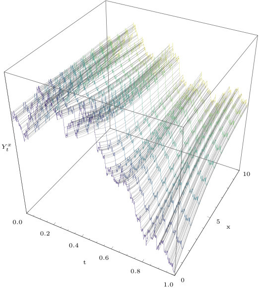 Figure 1
Peer Reviews
No public reviews on file for this paper yet. If you reviewed it on a platform where reviews are public (OpenReview, ICLR, NeurIPS, ICML), you can paste yours below so the community can read it here.
Videos
No videos yet. Explain this paper in a talk, walkthrough, or lecture? Add one.
Strong convergence rates for Markovian representations of fractional processes
Philipp Harms
Department of Stochastics
University of Freiburg
Abstract.
Many fractional processes can be represented as an integral over a family of Ornstein–Uhlenbeck processes. This representation naturally lends itself to numerical discretizations, which are shown in this paper to have strong convergence rates of arbitrarily high polynomial order. This explains the potential, but also some limitations of such representations as the basis of Monte Carlo schemes for fractional volatility models such as the rough Bergomi model.
2010 Mathematics Subject Classification:
60G22, 60G15, 65C05, 91G60
The author gratefully acknowledges support in the form of a Junior Fellowship of the Freiburg Institute of Advances Studies.
Contents
- 1 Introduction
- 2 Setting and notation
- 3 Integral representation
- 4 Discretization
- 5 Rough Bergomi model
- 6 Main result
- A Auxiliary results
1. Introduction
This paper establishes strong convergence rates for certain numerical approximations of fractional processes. These approximations are inspired by Markovian representations of fractional Brownian motion [14, 15, 31, 26] and of more general Volterra processes with singular kernels [32, 4, 2, 3, 16]. The simplest such representation takes the form
[TABLE]
where is standard Brownian motion, is Volterra Brownian motion111Also known as Riemann–Liouville fractional Brownian motion or Lévy’s definition of fractional Brownian motion. with Hurst index , and is an Ornstein–Uhlenbeck process with speed of mean reversion . The random field , which is depicted in Figure 1, has a version which is Hölder continuous in and smooth in ; see Lemma 1 for the precise statement. Thanks to this spatial smoothness, the integral can be approximated efficiently using high-order quadrature rules, following and extending [15, 26, 1, 3]. This leads to numerical approximations of the Volterra Brownian motion .
The main result of this article is that Volterra Brownian motion can be approximated at arbitrarily high polynomial convergence rates by weighted sums of Ornstein–Uhlenbeck processes; see Theorem 1 for the precise statement and error criterion. By arbitrarily high polynomial convergence rates we mean that -point interpolatory quadrature on suitably chosen spatial quadrature intervals leads to a discretization error of order for all ; see Remark 3. Thus, a given rate can be achieved by choosing . Note that low Hurst indices require high spatial quadrature orders to achieve a given approximation rate . A visual impression of the quality of this approximation can be obtained from Figure 2. The upper bound on the convergence rate closely matches the numerically observed rate; see Figure 3.
The motivation of this article is to develop efficient Monte Carlo methods for fractional (or rough) volatility models [24, 7, 11, 8, 27], which have been introduced on the grounds of extensive empirical evidence [24, 7, 11] and theoretical results [6, 20, 19, 9]. Under our discretization, put prices in the rough Bergomi model converge at the same rate as the underlying fractional volatility process; see Theorem 1. By put-call parity, this extends to call prices if the the asset and volatility processes are driven by negatively correlated Brownian motions, as explained at the end of Remark 2. A fully discrete Monte Carlo scheme for the rough Bergomi model can be obtained by discretizing the Ornstein–Uhlenbeck processes of Theorem 1 in time. This can be done efficiently because the covariance matrix of the Ornstein–Uhlenbeck increments has low numerical rank if the time steps are small.
To evaluate the computational complexity of our method, we consider the task of sampling a fractional process with Hurst index at a temporal grid of equidistant time points. Our method has some additional parameters, which determine the spatial discretization of the integral representation, namely the number of spatial quadrature intervals and the order of the spatial quadrature. These are described in detail in Lemma 2. On the above-mentioned task, our method achieves accuracy at complexity if the order of spatial quadrature is sufficiently high, i.e., if (see Remark 3). Equivalently, accuracy can be achieved at complexity , as stated in Table 1. Typically, one is interested in temporal grids of size for some . For instance, a value of slightly above guarantees that the piecewise constant interpolation of an -accurate time-discrete approximation defines a continuous-time approximation of the same order of accuracy in the supremum norm. This is because the sample paths of the fractional process are nearly -Hölder continuous. Under the assumption , Table 1 shows that our method outperforms the methods Hosking and Dieker [28, 17] and Carmona, Coutin, and Montseny [15] but is outperformed by the hybrid scheme of Bennedsen, Lunde, and Pakkanen [12] and by the circulant embedding method of Dietrich and Newsam [18]. This can be verified by substituting in Table 1. Using exponentially converging quadrature rules such as Chebychev [22, 21], one could at best hope to reduce the complexity of our method from down to . In the important special case with , this would result in exactly the same the complexity as the hybrid scheme [12] and the circulant embedding method [18].
Several directions for future generalization and improvement come to mind. Theorem 1 is proved by approximation in the Laplace domain, which implies convergence in the time domain by the continuity of the Laplace transform. As Volterra processes with Lipschitz drift and volatility coefficients depend continuously on the kernel in the norm, it would be interesting to check if similar convergence results hold also in this more general setting. The rate of convergence could potentially be improved using Chebychev quadrature, taking advantage of the real analyticity of the random field in the spatial variable . Finally, following [12, 30], one could aim for more careful treatments of the singularity of the kernel near the diagonal and apply some variance reduction techniques.
2. Setting and notation
We will frequently make the following assumptions. Let , let , let be the sigma-finite measure on the interval , let , let , let be a stochastic basis, and let be -Brownian motions.
3. Integral representation
Recall from the introduction that Volterra Brownian motion can be lifted to a random field indexed by a temporal variable and a spatial variable [14, 15, 31, 26]. The following lemma constructs a version of this random field which is continuous in the temporal variable and smooth in the spatial variable. Moreover, it establishes bounds on the spatial derivatives and tails of the random field. These bounds are needed for the subsequent error analysis in Section 4.
The constants appearing in Lemma 1 are used consistently throughout the paper: stands for the number of quadrature points in Definition 1 below, denotes the Hurst index shifted by one half, describes spatial integrability of , describes the integrability of the tail of as , and describes the integrability of the tail of as . The spaces of continuous, smooth, and integrable functions appearing in Lemma 1 carry their natural topologies and Borel sigma algebras; see Appendix A.
Lemma 1**.**
Assume the setting of Section 2.
- (a)
There exists a measurable mapping
[TABLE]
such that
[TABLE] 2. (b)
Volterra Brownian motion is a linear functional of in the sense that
[TABLE] 3. (c)
The following integrability conditions hold: for all , , , and ,
[TABLE]
Proof.
(a) By
[TABLE]
defines a measurable map
[TABLE]
(b) follows from the above and the stochastic Fubini theorem [34]: for each , one has almost surely that
[TABLE]
(c) Let be the constant in the maximal inequality for Ornstein–Uhlenbeck processes (see Lemma 5), i.e.,
[TABLE]
Recall that , and define as
[TABLE]
By the inequality , one obtains the following three estimates:
[TABLE]
This shows (c) for . The generalization to is immediate because the norms of a Banach-valued Gaussian random variable are mutually equivalent thanks to the Kahane–Khintchine inequality [33, Theorem V.5.3] applied to the Karhunen–Loève expansion [33, Theorem V.5.7]. ∎
4. Discretization
In this section, the measure in the integral representation of Volterra Brownian motion is approximated by a weighted sum of Dirac measures. More specifically, for each , the positive half line is truncated to a finite interval . This interval is then split into subintervals by a geometric sequence , and on each subinterval the measure is approximated by an -point interpolatory quadrature rule such as e.g. the Gauss rule. Classical error analysis for interpolatory quadrature rules (see e.g. [13]) then yields the desired convergence result.
Definition 1**.**
Let satisfy , let be a continuous function such that , and let . Then a measure on is called a non-negative -point interpolatory quadrature rule on with respect to the weight function if there are grid points and weights such that and
[TABLE]
The following lemma discretizes the integral representation of Volterra Brownian motion using interpolatory quadrature rules and bounds the discretization error. The assumptions of the lemma are satisfied thanks to the bounds of Lemma 1, where the same constants are used.
Lemma 2**.**
Assume the setting of Section 2, let and satisfy , let
[TABLE]
be a measurable function which satisfies the integrability conditions
[TABLE]
let , for each and let
[TABLE]
let be a non-negative -point interpolatory quadrature rule on with respect to the weight function , and let . Then
[TABLE]
Proof.
We define the constants
[TABLE]
where the upper bound on follows from Bernoulli’s inequality
[TABLE]
the finiteness of follows from the inequality
[TABLE]
and the finiteness of follows from the fact that tends to zero as . Recall that the measures are by assumption non-negative -point interpolatory quadrature rules. Therefore, the corresponding quadrature error can be expressed as follows [13, Theorem 4.2.3]: for each , , and , one has
[TABLE]
where the Peano kernel is a measurable function which satisfies [13, Theorem 5.7.1]
[TABLE]
Thus, one has for each that
[TABLE]
This can be expressed as a geometric series: letting , one has for each that
[TABLE]
Absorbing the denominator into one of the factors and discarding the term yields for each that
[TABLE]
For each , this can be estimated by
[TABLE]
Therefore, noting that , one has
[TABLE]
Remark 1**.**
The choice of the quadrature rule in Lemma 2 is admittedly somewhat arbitrary but produces good results. The use of the geometric grid goes back to [15] and simplifies the error analysis compared to more complex subdivisions which distribute the error more equally. It would be interesting to explore if the holomorphicity of permits the use of quadrature rules with exponential convergence rates such as Chebychev quadrature; see the discussion in Section 3.
5. Rough Bergomi model
The following lemma establishes that prices of put options in the rough Bergomi model converge at the same rate as the approximated Volterra processes. This holds not only for the Ornstein–Uhlenbeck approximations of Lemma 2, but more generally for any approximation of the log-volatility in the norm. Below, the space of real-valued Lipschitz functions is denoted by and endowed with the norm .
Lemma 3**.**
Assume the setting of Section 2, let be continuous stochastic processes with and
[TABLE]
and let be a measurable function such that . Then
[TABLE]
Proof.
It is sufficient to control the log prices in because
[TABLE]
The basic inequality
[TABLE]
and the Burkholder–Davis–Gundy inequality [10, Theorem 1.2] imply that
[TABLE]
Remark 2**.**
For each the put-option payoff
[TABLE]
satisfies the assumption of Lemma 3 that because
[TABLE]
The call-option payoff does not have this property, but the prices of call options can be obtained by put-call parity if and are negatively correlated because this implies that is a martingale [23].
6. Main result
The following theorem combines the analyses of Lemmas 1–3 to show that Volterra Brownian motion can be approximated numerically at arbitrarily high polynomial convergence rates . The same convergence rate is inherited by the associated put prices in the rough Bergomi model.
Theorem 1**.**
Assume the setting of Section 2. For any given , the following statements hold:
- (a)
Volterra Brownian motion can be approximated at rate by a sum of Ornstein–Uhlenbeck processes in the following sense: for each there are speeds of mean reversion and weights , , such that the continuous versions and of the stochastic integrals
[TABLE]
satisfy
[TABLE] 2. (b)
Under the above approximation, put prices in the rough Bergomi model converge at rate in the following sense: the processes and defined for all and by
[TABLE]
satisfy for all strikes that
[TABLE]
Proof.
(a) follows from the integral representation in Lemma 1 and its discretization in Lemma 2. More precisely, the -point quadrature rule in Lemma 2 converges at any rate , where the parameters , , , and are as in Lemma 1. The speeds of mean reversion and weights are determined by the relation , where is as in Lemma 2. Moreover, (b) follows from (a) and Lemma 3. ∎
Remark 3**.**
The proof of Theorem 1 shows that -point interpolatory quadrature on suitably chosen spatial quadrature intervals leads to a discretization error of order for all .
Appendix A Auxiliary results
The space of continuous real-valued functions on an interval is Banach with the supremum norm. Moreover, the space of smooth real-valued functions on is locally convex with the family of seminorms , where runs through the compact subsets of and through the natural numbers. Similarly, the space is locally convex with the family of seminorms for and as before.
Lemma 4**.**
Assume the setting of Section 2. Then the following function is continuous:
[TABLE]
Proof.
It is sufficient to show for each and each compact that the following mapping is continuous:
[TABLE]
This is obvious because this is a bounded linear map between Banach spaces. ∎
The following maximal inequality for Ornstein–Uhlenbeck processes has been shown by [25, Theorem 2.5 and Remark 2.6].
Lemma 5**.**
Assume the setting of Section 2. For each , let be a measurable map such that
[TABLE]
Then there exists a universal constant such that the following maximal inequality holds:
[TABLE]
The following result has been shown in [26, Theorem 2.11]. We reproduce the argument here and give a simpler proof of measurability. Recall from Section 2 that is a sigma-finite measure on and that, accordingly, the space of -integrable functions is a separable Banach space. Its intersection with the locally convex space is again locally convex with the union of the corresponding families of seminorms.
Lemma 6**.**
Assume the setting of Section 2, and let be a measurable map such that
[TABLE]
Then almost surely takes values in the space and is measurable as a map
[TABLE]
Proof.
The expression
[TABLE]
is well-defined thanks to the continuity in of , and is finite thanks to Lemma 5. Thus, the dominated convergence theorem implies that has continuous sample paths in . It remains to show that is measurable. As the Borel sigma algebra on is generated by point evaluations at [5, Lemma 4.53], it suffices to show for each that is measurable. Moreover, by Pettis’ measurability theorem [29, Proposition 1.1.1] and the separability of , it suffices to show that is weakly measurable, i.e., that is measurable for each . This follows by approximation
[TABLE]
where for each , is a sequence of atomic signed measures on the interval which converges weakly to the signed measure on the same interval. ∎
The reference list from the paper itself. Each links out to its DOI / PubMed record.
- 1[1] Eduardo Abi Jaber “Lifting the Heston model” In Quantitative Finance 19.12 Taylor & Francis, 2019, pp. 1995–2013
- 2[2] Eduardo Abi Jaber and Omar El Euch “Markovian structure of the Volterra Heston model” In Statistics & Probability Letters 149 Elsevier, 2019, pp. 63–72
- 3[3] Eduardo Abi Jaber and Omar El Euch “Multifactor approximation of rough volatility models” In SIAM Journal on Financial Mathematics 10.2 SIAM, 2019, pp. 309–349
- 4[4] Eduardo Abi Jaber, Martin Larsson and Sergio Pulido “Affine volterra processes” In The Annals of Applied Probability 29.5 Institute of Mathematical Statistics, 2019, pp. 3155–3200
- 5[5] Charalambos D. Aliprantis and Kim C. Border “Infinite dimensional analysis. A Hitchhiker’s guide” Springer, 2006
- 6[6] Elisa Alòs, Jorge A León and Josep Vives “On the short-time behavior of the implied volatility for jump-diffusion models with stochastic volatility” In Finance and Stochastics 11.4 Springer, 2007, pp. 571–589
- 7[7] Christian Bayer, Peter Friz and Jim Gatheral “Pricing under rough volatility” In Quantitative Finance 16.6 Taylor & Francis, 2016, pp. 887–904
- 8[8] Christian Bayer et al. “A regularity structure for rough volatility” In Mathematical Finance 30.3 Wiley Online Library, 2020, pp. 782–832