TL;DR
This paper presents a realistic, real-time quad-rotor flight simulation framework that incorporates advanced atmospheric models and validated aerodynamics, enabling improved trajectory planning and control in low-altitude conditions.
Contribution
It introduces an integrated simulation environment combining validated aerodynamic models, atmospheric boundary layer simulations, and nonlinear control for quad-rotors, with open-source code for community use.
Findings
Wind model accuracy significantly affects trajectory predictions.
Simplified rotor aerodynamics impact flight performance.
Open-source simulation tools facilitate research and development.
Abstract
In trajectory planning and control design for unmanned air vehicles, highly simplified models are typically used to represent the vehicle dynamics and the operating environment. The goal of this work is to perform real-time, but realistic flight simulations and trajectory planning for quad-copters in low altitude (<500m) atmospheric conditions. The aerodynamic model for rotor performance is adapted from blade element momentum theory and validated against experimental data. Large-eddy simulations of the atmospheric boundary layer are used to accurately represent the operating environment of unmanned air vehicles. A reduced-order version of the atmospheric boundary layer data as well as the popular Dryden model are used to assess the impact of accuracy of the wind field model on the predicted vehicle performance and trajectory. The wind model, aerodynamics and control modules are…
Click any figure to enlarge with its caption.
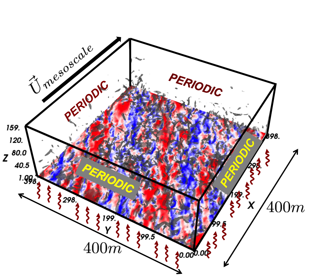 Figure 1
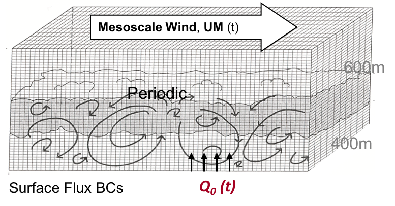 Figure 2
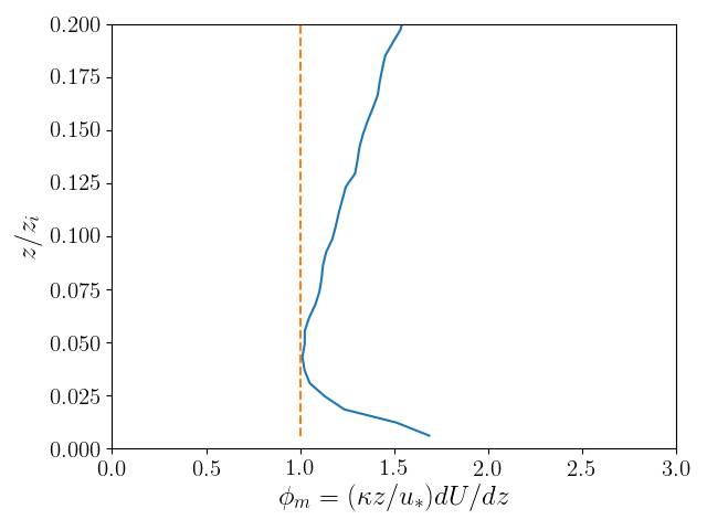 Figure 3
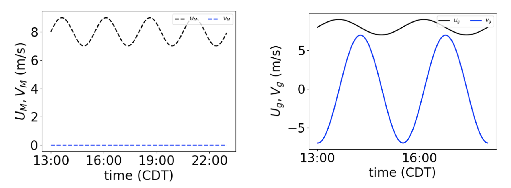 Figure 4
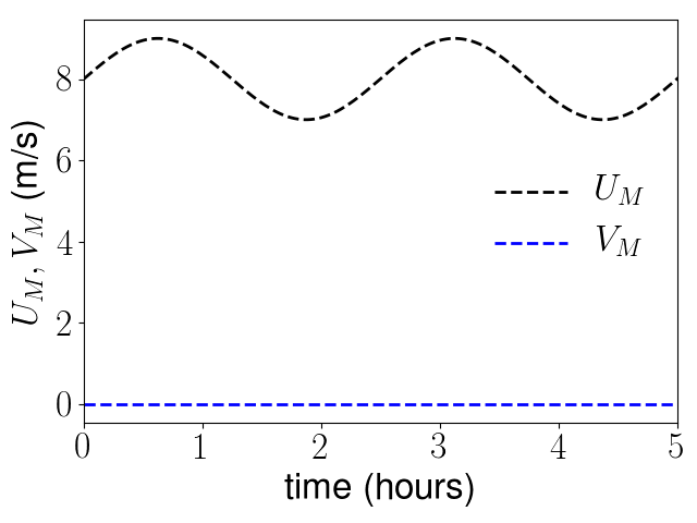 Figure 5
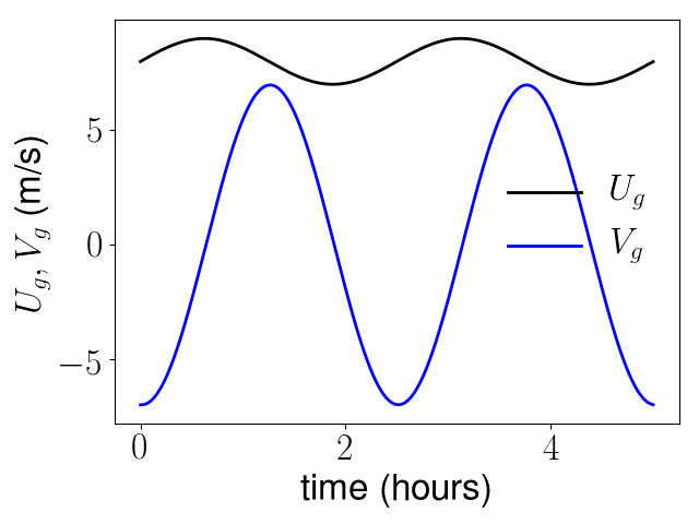 Figure 6
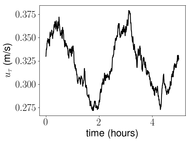 Figure 7
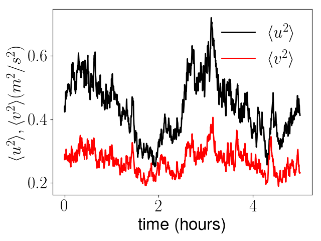 Figure 8
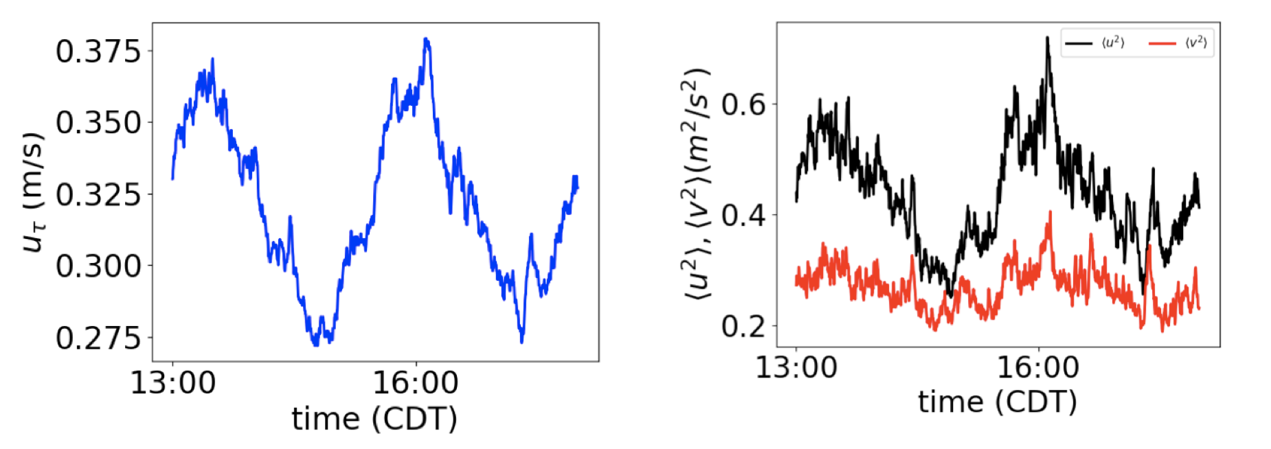 Figure 9
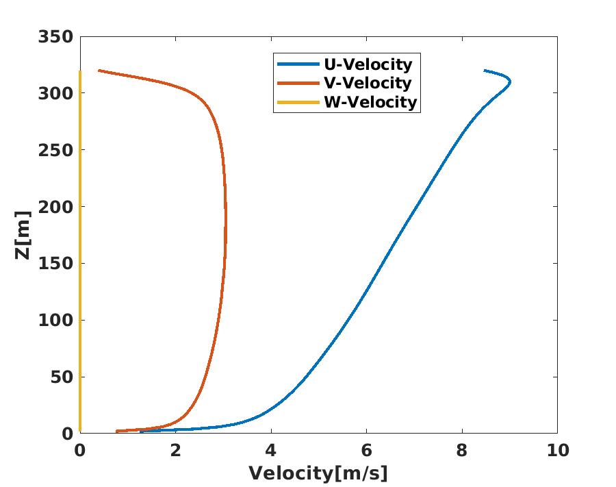 Figure 10
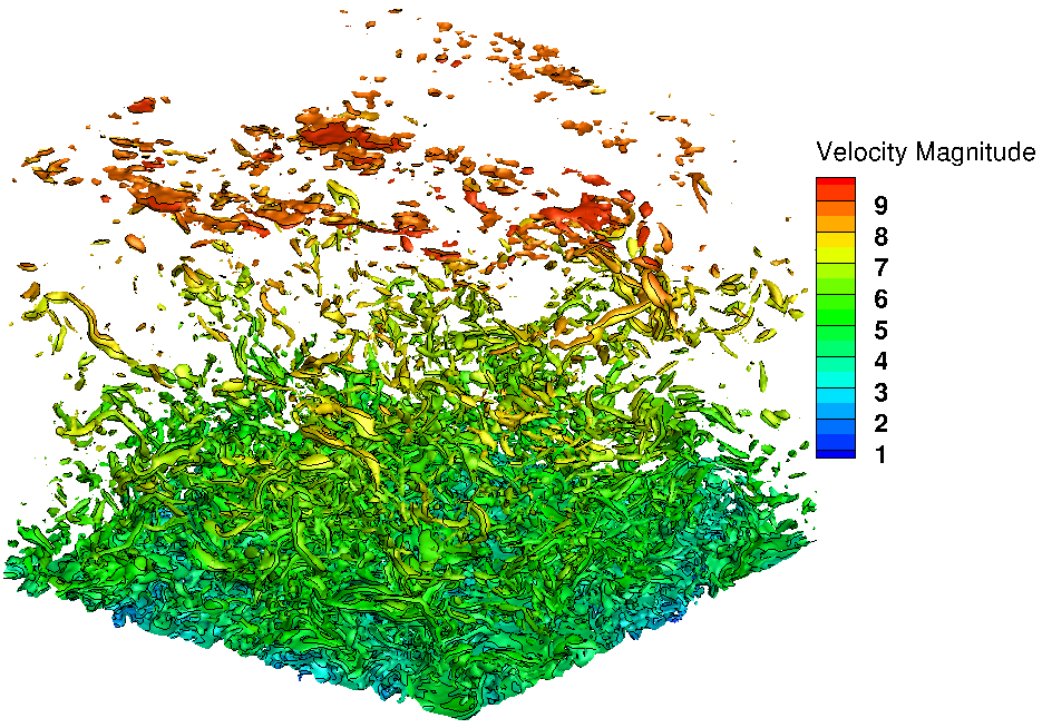 Figure 11
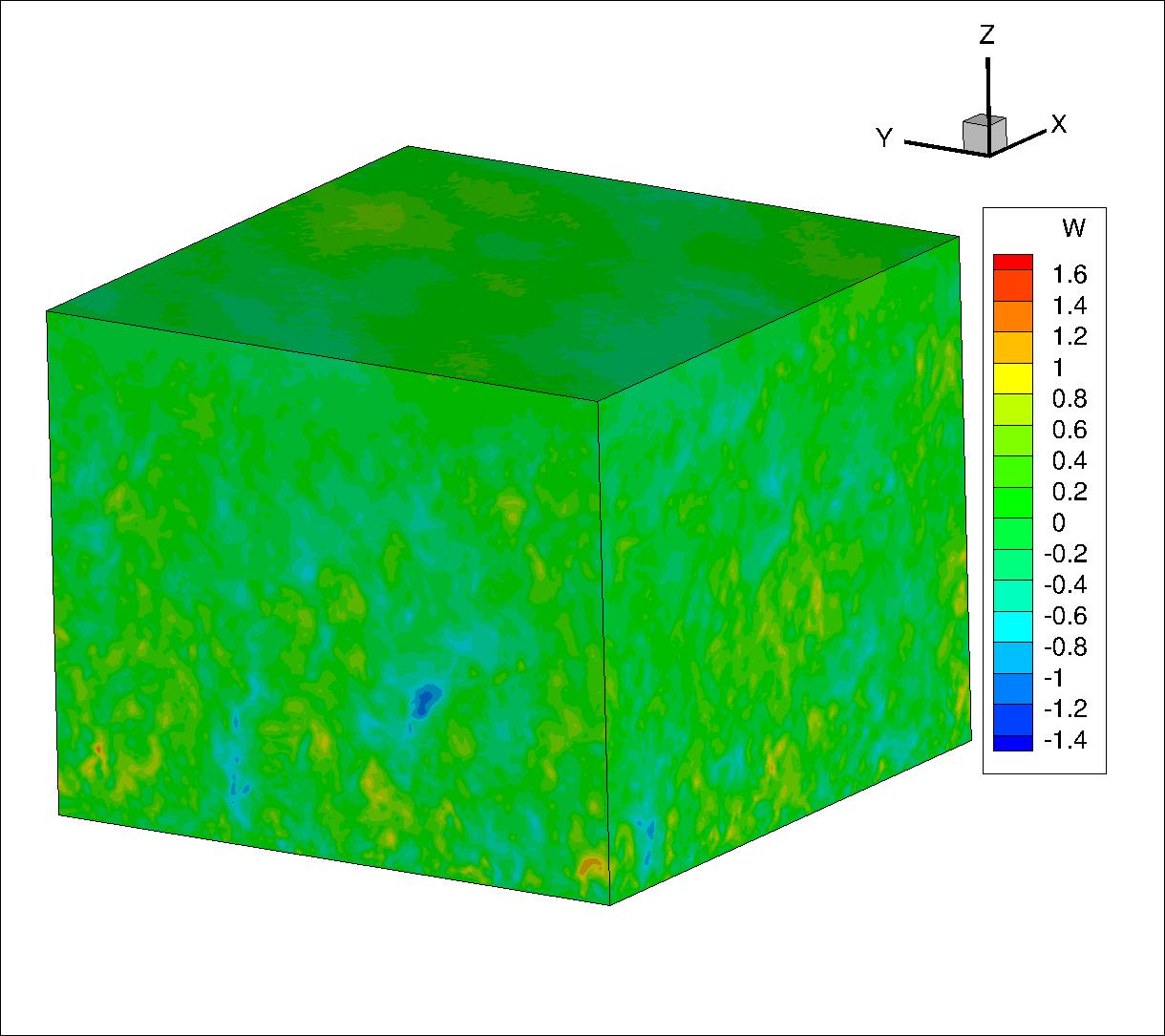 Figure 12
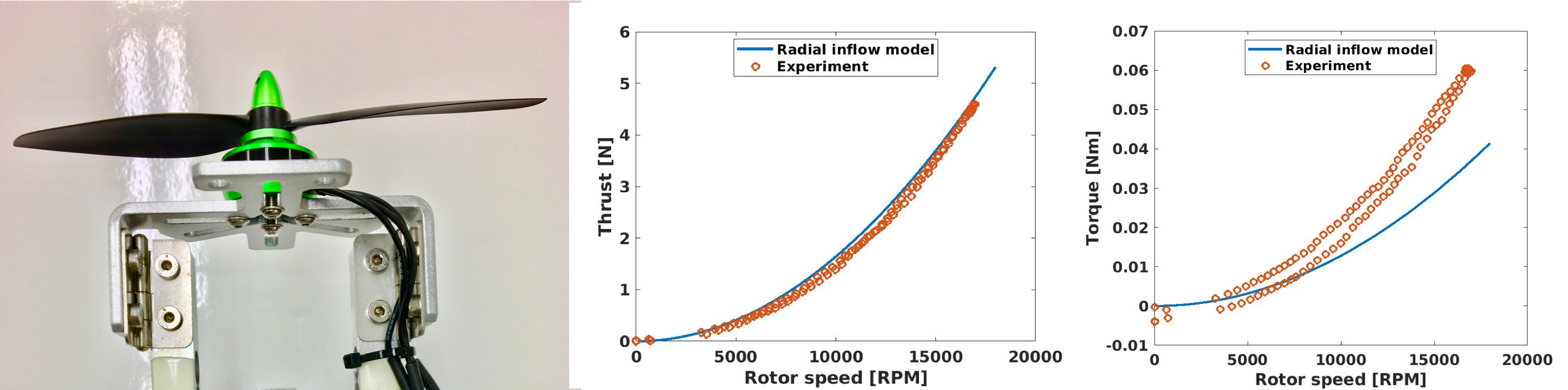 Figure 13
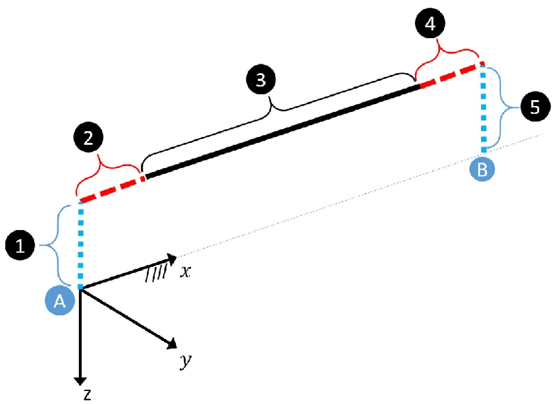 Figure 14
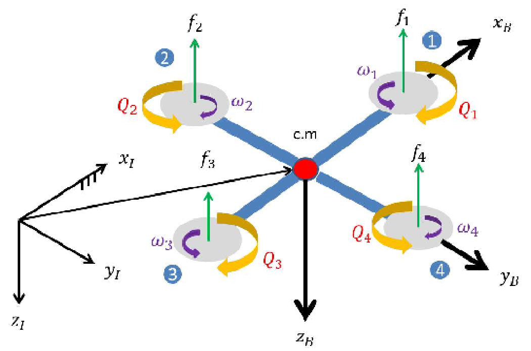 Figure 15
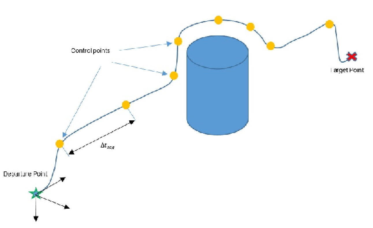 Figure 16
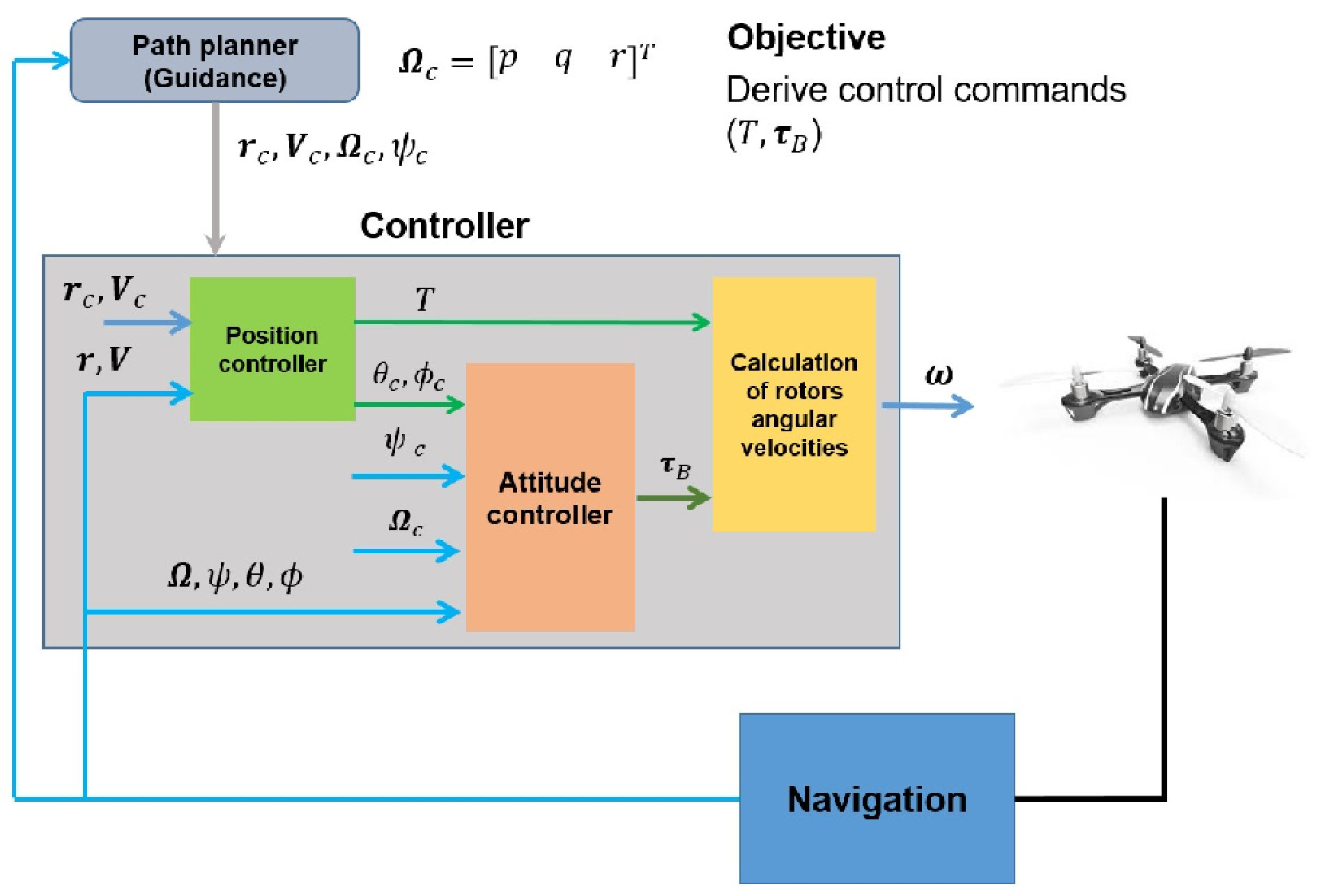 Figure 17
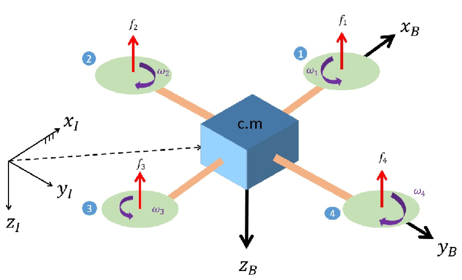 Figure 18
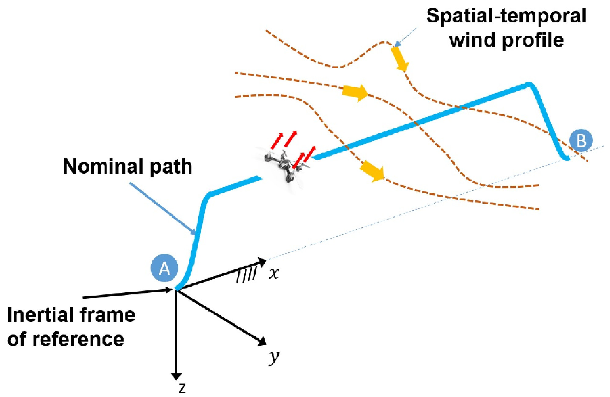 Figure 19
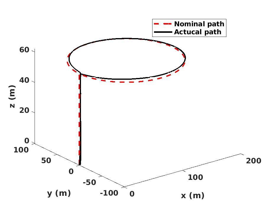 Figure 20
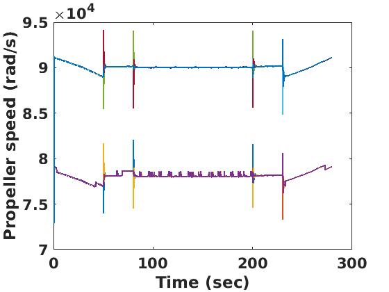 Figure 21
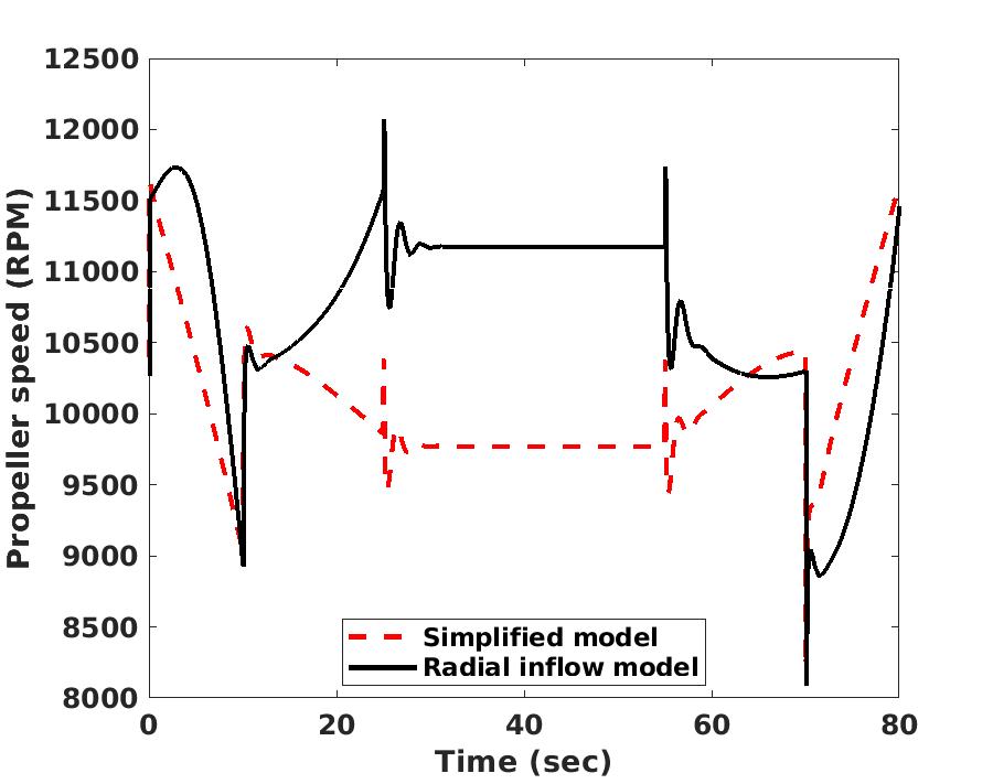 Figure 22
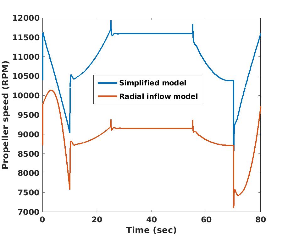 Figure 23
 Figure 24
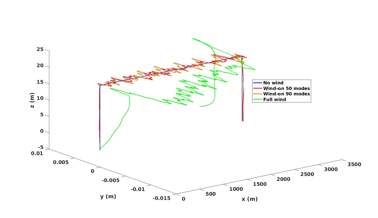 Figure 25
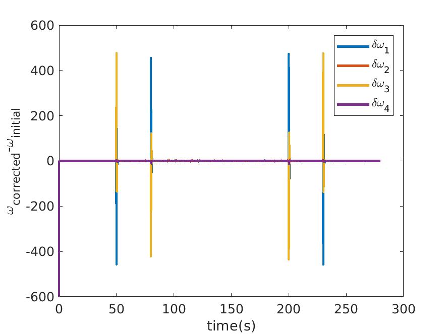 Figure 26
 Figure 27
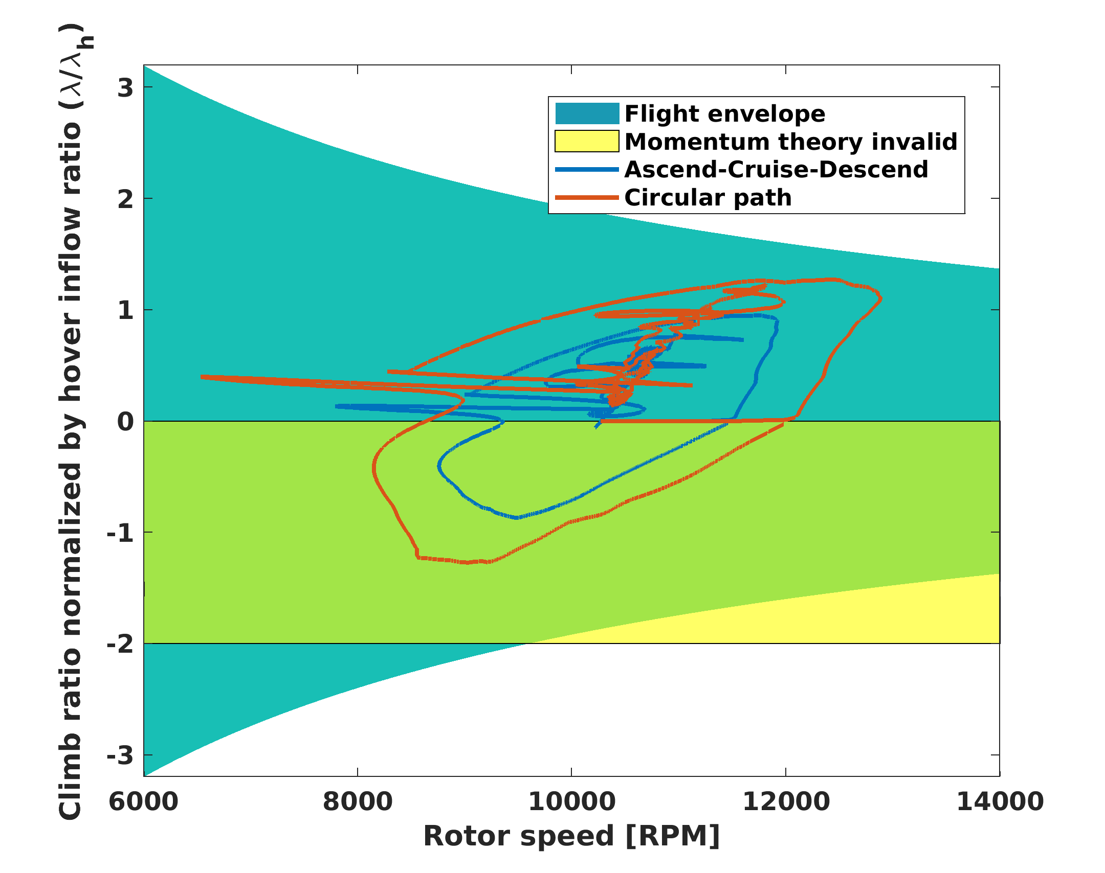 Figure 28
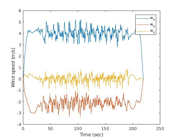 Figure 29
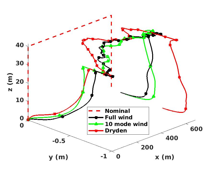 Figure 30
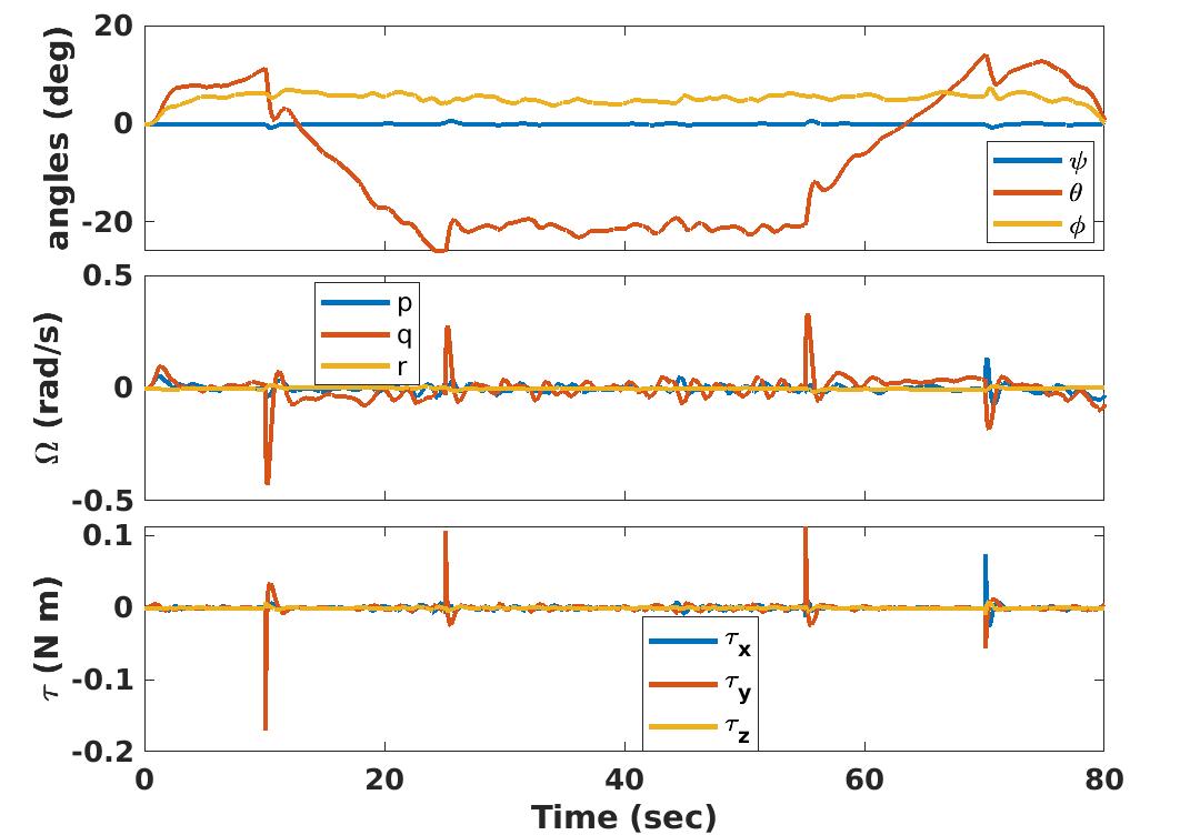 Figure 31
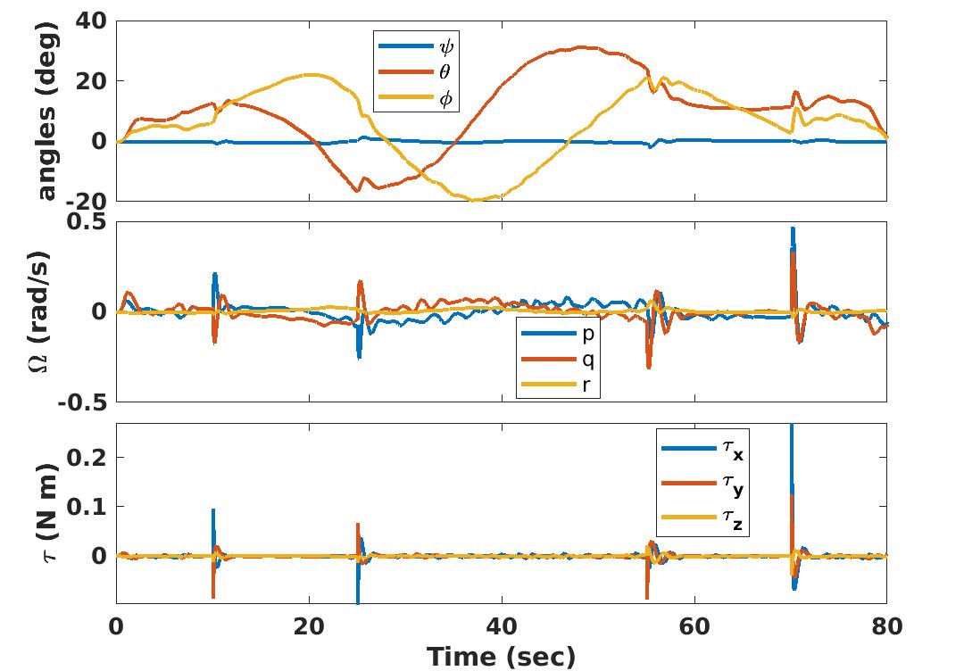 Figure 32
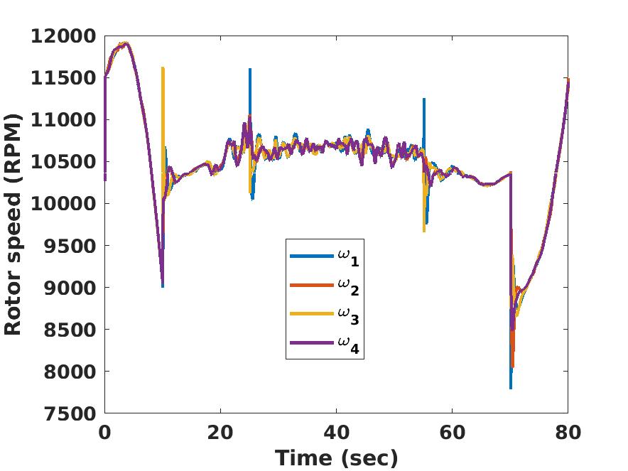 Figure 33
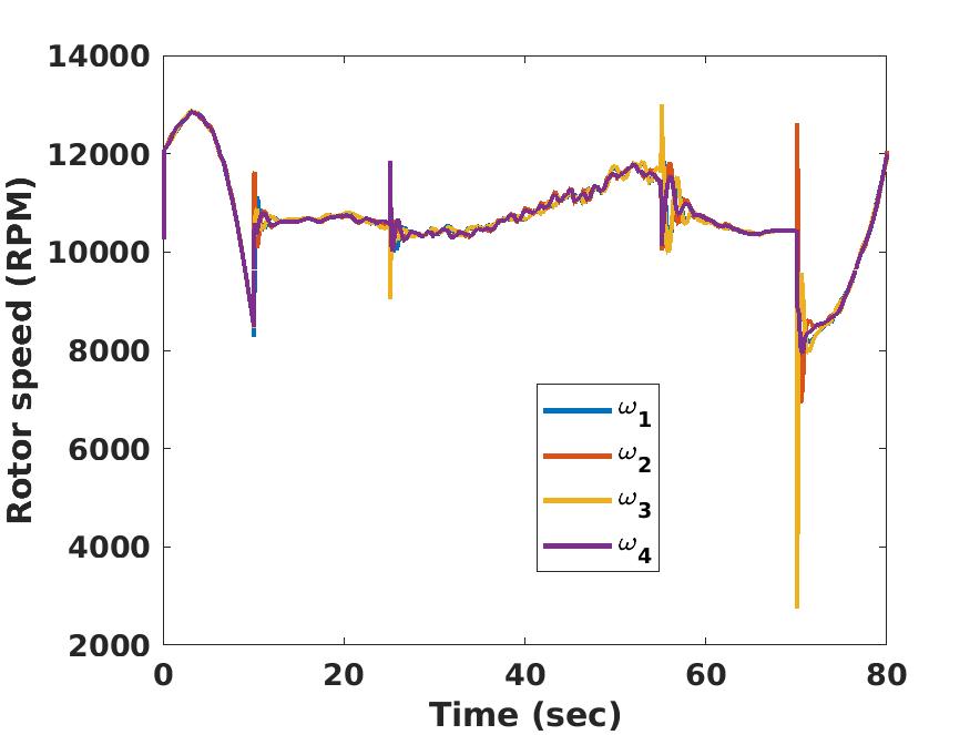 Figure 34
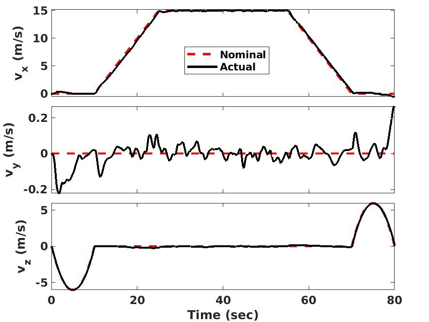 Figure 35
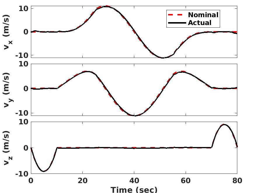 Figure 36
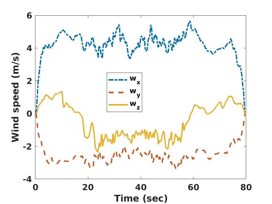 Figure 37
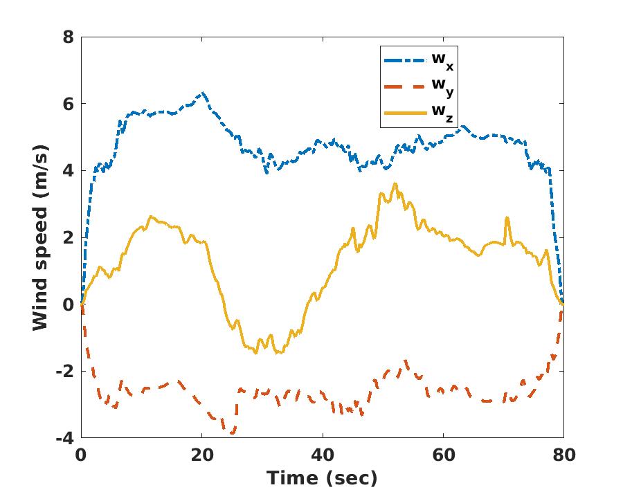 Figure 38
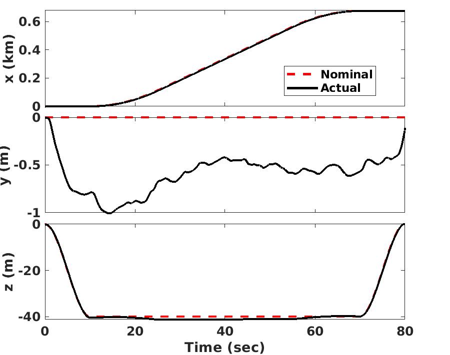 Figure 39
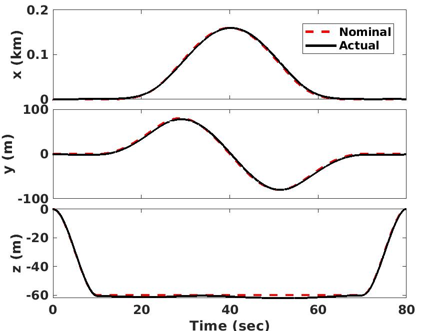 Figure 40
Peer Reviews
No public reviews on file for this paper yet. If you reviewed it on a platform where reviews are public (OpenReview, ICLR, NeurIPS, ICML), you can paste yours below so the community can read it here.
Code & Models
Videos
No videos yet. Explain this paper in a talk, walkthrough, or lecture? Add one.
Quad-rotor Flight Simulation in Realistic Atmospheric Conditions
Behdad Davoudi111PhD Candidate.
Ehsan Taheri222Post Doctoral Fellow, currently Research Assistant Professor, Texas A&M University.
Karthik Duraisamy333Associate Professor.
Balaji Jayaraman444Visiting Researcher, currently Assistant Professor of Mech. & Aero. Eng., Oklahoma State University.
Ilya Kolmanovsky555Professor.
Department of Aerospace Engineering, University of Michigan, Ann Arbor, MI 48109
Abstract
In trajectory planning and control design for unmanned air vehicles, highly simplified models are typically used to represent the vehicle dynamics and the operating environment. The goal of this work is to perform real-time, but realistic flight simulations and trajectory planning for quad-copters in low altitude (<500m) atmospheric conditions. The aerodynamic model for rotor performance is adapted from blade element momentum theory and validated against experimental data. Large-eddy simulations of the atmospheric boundary layer are used to accurately represent the operating environment of unmanned air vehicles. A reduced-order version of the atmospheric boundary layer data as well as the popular Dryden model are used to assess the impact of accuracy of the wind field model on the predicted vehicle performance and trajectory. The wind model, aerodynamics and control modules are integrated into a six-degree-of-freedom flight simulation environment with a fully nonlinear flight controller. Simulations are performed for two representative flight paths, namely, straight and circular paths. Results for different wind models are compared and the impact of simplifying assumptions in representing rotor aerodynamics is discussed. The simulation framework and codes are open-sourced for use by the community.
Nomenclature
[TABLE]
[TABLE]
I Introduction
Over the past decade, small Unmanned Aerial Systems (sUAS) (or drones) cai2014survey have been increasingly utilized in a variety of tasks including rapid package delivery lee2017optimization , border patrolling wall2011surveillance , damage inspection irizarry2012usability , disaster management adams2011survey , mapping nex2014uav , precision agriculture zhang2012application , etc. With the unprecedented growth in the number of flight vehicles, simulation tools are required for trajectory prediction and validation, especially in the context of certification by analysis.
A representative trajectory for a quad-copter is shown in Figure 1 where the vehicle is assigned, for instance, with a package delivery task. It dispatches from point ‘A’ (say a service center) to point ‘B’ (that may represent a delivery designated area) on a nominal trajectory.
The quad-copter is subject to extraneous factors such as wind/gusts that affects its performance and trajectory and may deviate its path from the planned one. In practice, there are various along-the-path constraints that have to be taken into consideration during path-planning, specifically, for very low-altitude flight since the quad-copter has to adopt certain maneuvers to avoid colliding with obstacles.
A comprehensive approach to validating and planning trajectories of flying vehicles requires, in general, a framework that takes into account various aspects including 1) appropriate-fidelity aeromechanical and dynamic models of the vehicle to present a realistic view of the actual motion, 2) accurate modeling of the environment, which may include modeling of external factors that alter the trajectory of the vehicle including wind and gust models, 3) development of a flight controller to control vehicle trajectory to within a prescribed accuracy, 4) a guidance (motion-planning) algorithm that provides a nominal “optimal” trajectory, and 5) a navigation model to represent the sensory data and the measurement noise, which will be used to update the location/orientation of the flying vehicle to be used for guidance and by the flight controller.
Depending on the stage and/or nature of the study, various simplifications are invoked to facilitate the task of trajectory prediction and performance analysis berning2018rapid . For instance, it is common to consider a three-degree-of-freedom model to only trace the trajectory of the center of mass of the vehicle while the orientation of the vehicle is considered to be of secondary importance for early analysis zipfel2007modeling . As another example, in launch vehicle or entry, descent and landing trajectory design/analysis, it is common to consider four degrees-of-freedom to trace the motion of the center of mass and the orientation of the body of the vehicle with respect to a reference direction, namely, the pitch angle mall2016trigonomerization . A similar approach is used for motion analysis of flying vehicles when only planar motion is assumed. The inclusion of additional degrees of freedom is usually considered for higher-fidelity models and at later stages of design of systems to gain better understanding of the motion and to obtain realistic flight performance envelopes desai2008six ; roshanian2014multidisciplinary ; kamyar2014aircraft .
Simplified atmospheric models are typically used for mission planning and certification of unmanned air vehicles (UAVs). In practice, the operating environment of UAVs flying at low altitudes ( m) is not only subject to strong mean velocity gradients (shear), but also involves intermittent unsteady wind gusts that contain a non-trivial fraction of energy compared to the mean flow. Further, the characteristic size of the turbulent eddies, even in a stable boundary layer, is of the order of a few meters kosovic2000large , which is similar to the size of an sUAS. Accounting for such scales becomes critical to the vehicle aeromechanics and thus to more accurate trajectory prediction and validation tasks.
A widely used tool for numerical weather prediction is the Weather Research and Forecasting (WRF) model wrf1 ; wrf2 . WRF is, however, a mesoscale model and is typically used over large spatial domains ( km) and with coarse resolutions ( km). WRF thus cannot be relied upon to represent all eddies and gusts of interest for sUAS trajectory prediction and validation purposes, and thus a different, higher resolution approach is required.
In addition, a critical element in performance and/or trajectory analysis of flying vehicles is to use accurate dynamical models for the propulsion system. For an airplane, this entails modeling of the engine/propellers, whereas for a quad- or multi-copter not only the individual performance of the propellers, but their mutual interactions become important, and have to be taken into consideration for certain types of maneuvers ventura2018high . In particular, the key requirement for the aeromechanics model is to provide an effective characterization of the response of a sUAS to unsteady gust loads sydney2013dynamic . An additional requirement is that the fidelity of the model should be such that it is easily integrable into the trajectory validation and planning modules and the necessary computations can be performed in near-real time.
It is common practice to approximate the actual performance of a propeller (i.e., the thrust or torque) using idealized, simple algebraic models to facilitate numerical analyses. The so-called static models (namely, the thrust and torque of a rotor are expressed in terms of the square of rotor speed) are used extensively for hovering, and slow maneuvers. However, these models do not capture the realistic performance of a propeller, which in general, depends on the inflow velocity. In particular, more accurate models have to be used for flight trajectories that can be utilized in demanding situations such as high speed forward and descent flight phases huang2009aerodynamics . In low-altitude flight, these aerodynamic phenomena can influence the vehicle dynamics in the presence of wind and gusts. Towards this end, a propeller thrust model in forward flight was presented in zhang2014survey for a blade with linear twist.
On the other hand, the use of higher-fidelity models such as those based on computational fluid dynamics ventura2018high ; lakshminarayan2006computational or even vortex-based methods kim2009interactional to predict the aeromechanics of flight vehicles is computationally demanding, and thus is not feasible in trajectory optimization or trajectory prediction settings. As a consequence, an additional challenge is to establish a set of computationally efficient and effective models of the aeromechanics and flight dynamics of the sUAS vehicles.
The main contribution of this paper is to present efficient and accurate models of atmospheric conditions and vehicle aeromechanics, with the goal of utilizing them in real-time trajectory planning, validation and control. Specifically, the operating environment is characterized via atmospheric boundary layer simulations. Aeromechanical models of appropriate fidelity are derived using momentum and blade element theories with an emphasis on low-altitude flight. These models are integrated with a numerical simulation environment that propagates a six-degree-of-freedom (6DoF) model of a quad-copter along two representative nominal flight trajectory profiles: 1) an ascent-straight-descent profile and 2) a circular path. In addition, the trajectory of the quad-copter is controlled using a fully non-linear backstepping control algorithm. Results from different wind models and propeller models are compared and discussed, highlighting the importance of modeling fidelity for realistic trajectory planning, validation and control.
The remainder of the paper is organized as follows. Section II introduces the atmospheric boundary layer model. Section III presents a review of the aerodynamic model. Section IV discusses the details of a fully nonlinear flight controller (namely, translational-rotational control algorithm). In Section V, the coupling between the aerodynamic models and control module is presented. Aerodynamic, dynamic, control and wind models are integrated, and flight simulation results for a variety of problems are performed and presented in Section VI. Section VII provides a summary and conclusions.
II Modeling Atmospheric Gust Effects
The popular approach to represent atmospheric gusts in aviation applications such as trajectory estimation relies on stochastic von1948progress ; MIL-STD1990 ; MIL-HDBK2012 formulations and models of the spectral energy function (and, in turn, the trace of the spectral energy tensor) pope2001turbulent . While computationally efficient, such methods have two major limitations: (i) use of parameterized equilibrium phenomenology that is often inaccurate, and (ii) not explicitly accounting for the structure of the spectral energy tensor. The components of the spectral energy tensor contain information about the anisotropy and coherence in the turbulence structure. In reality, the atmospheric boundary layer (ABL) turbulence is characterized by strong and highly coherent eddying structure that contributes to the uncertainty associated with the predicted trajectory. In this study, we adopt high fidelity Large Eddy Simulations (LES) of the ABL that accurately represent energy containing turbulence eddying structures at scales that are dynamically important for unmanned aerial flight.
The canonical ABL used to generate the wind model data for this study is modeled as a rough flat wall boundary layer with surface heating from solar radiation, forced by a geostrophic wind in the horizontal plane and solved in the rotational frame of reference fixed to the earth’s surface. The lower troposphere that limits the ABL to the top is represented with a capping inversion and the mesoscale effects through a forcing geostrophic wind vector. In fact, the planetary boundary layer is different from engineering turbulent boundary layers in three major ways: 1) Coriolis Effect: The rotation of the earth causes the surface to move relative to the fluid in the ABL, which results in angular displacement of the mean wind vector that changes with height, 2) Buoyancy-driven turbulence: The diurnal heating of the surface generates buoyancy-driven temperature fluctuations that interact with the near-surface turbulent streaks to produce turbulent motions, and 3) Capping Inversion: A layer with strong thermal gradients that caps the microscale turbulence from interacting with the mesoscale weather eddies.
In Figure 2, the mesoscale wind drives the ABL along the x-direction while the rotation of the earth’s surface orients the surface layer turbulence to nearly degrees relative to the imposed wind vector (along the streaks). The isosurfaces (grey) show vorticity magnitude at a value of and the isocontours show the horizontal fluctuating velocity. The blue regions denote low speed streaks while the red regions represent high speed streaks.
II.0.1 LES Methodology and Simulation Design:
The Reynolds number of the daytime atmospheric boundary layer is extremely large. Hence, only the most energetic atmospheric turbulence motions are resolved. The eddies in the surface layer are highly inhomogeneous in the vertical (z), but are clearly homogeneous in the horizontal direction. LES attempts to resolve to the order of the grid scale, the energy containing eddy structures.
Using a grid filter, one can split the fluctuating instantaneous velocity and potential temperature into a resolved and sub-filter scale (SFS) components. The canonical, quasi-stationary equilibrium ABL is driven from above by the horizontal mesoscale ‘geostrophic wind’ velocity vector, , and the Coriolis force is converted into a mean horizontal pressure gradient oriented perpendicular to . In the LES of ABL, the molecular viscous forces are neglected and the surface roughness elements of scale are not resolved by the first grid cell . Buoyancy forces are accurately predicted using the Boussinesq approximation. The momentum equation for resolved velocity contains a sub-filter scale (SFS) stress tensor that is modeled using an eddy viscosity formulation with the velocity scale being generated through a 1-equation formulation for the SFS turbulent kinetic energy moeng1984large ; moeng1986large . The LES equations are shown below in Eqns. (1)-(3). A detailed discussion of the numerical methods is available in khanna1997analysis ; jayaraman2014transition ; jayaraman2018transition . In the equations below, represents the filtered velocity, the subfilter scale stresses, the modified pressure and the filtered potential temperature.
[TABLE]
While the effects of buoyancy are highly pronounced in ABL turbulence, and significantly impact its structure jayaraman2014transition ; jayaraman2018transition , we chose a more benign neutral stratification for this study. To pack sufficient resolution to capture scales relevant to small fixed wind unmanned vehicles, we restricted the domain size to . The cartesian LES grid has a resolution of for a uniform spacing of 2m in each spatial direction. To realistically mimic the interface between the mesoscale and microscale atmospheric turbulence, a capping inversion was specified at a height of 280m. The surface heat flux is set to zero for this neutral ABL simulation and a Coriolis parameter of is chosen to represent continental United States. The bottom surface is modeled as uniformly rough with a characteristic roughness scale of 16cm that is typical of grasslands. The dynamical system described in Eqs. (1)-(3) is forced by an impossed mean pressure gradient, usually specified in terms of a geostrophic wind as . For this model, is set to 8m/s which corresponds to a moderately windy day. The equation system is solved using the pseudo-spectral method in the horizontal with periodic boundary conditions and second-order finite difference in the vertical. The time marching is accomplished using a third-order Runge-Kutta method. The computational set-up is exactly as shown in Figure. 2. Further details about the computational methods and models can be obtained from jayaraman2014transition ; jayaraman2018transition ; khanna1997analysis .
II.0.2 Validation of Results
The LES framework has been validated for equilibrium conditions with experimental data johansson2001critical and well known phenomenology khanna1997analysis in the past and is well established as a high fidelity bench tool for modeling near surface atmospheric flows. In this study, we adopt a similar strategy and assess the non-dimensional near-wall scaling from simulation data with respect to the law of the wall, and Monin-Obukhov (M-O) similarity theory arguments for neutral stratification. Particularly, we compute the non-dimensional mean gradient which should be closer to unity in the inertial logarithmic region of the ABL. In the above, the non-dimensionalization is performed using the appropriate choice of near-surface parameters for length (distance from the wall, ) and velocity (friction velocity, ). For a constant value of the mesoscale wind and surface heat flux, the turbulent flow field evolves into a fully developed equilibrium boundary layer. After verifying the existence of statistical stationarity, converged statistics were plotted. Fig. 3 shows the near-wall variation of as a function of normalized distance from the surface, (), where is the height of the ABL. We observe that assumes values closer to unity with deviations known to arise from a combination of inaccuracies in the assumed value of the von Karman constant, , numerical errors and near-wall modeling, which introduces an artificial numerical viscous length scale brasseur2010designing . The LES is considered acceptable as long as these deviations are small as observed in this case.
II.0.3 Non-stationary ABL Turbulence
While the above discussion focuses on modeling equilibrium turbulence, the realistic wind fields observed in the atmosphere is often not in equilibrium. Such deviations from equilibrium arise due to multiple reasons including diurnal variations, spatial heterogenieties, terrain and influence of nonstationary mesoscale wind events. To assess the influence of some of these effects on the turbulence structure, we incorporate non-stationary, slow-varying sinusoidal wind (period of O(hours)) on a neutral ABL. This forcing strategy follows the earlier work on mesi-micro coupling by Jayaraman and co-authors in jayaraman2014nonequilibrium . The LES design for this simulation is the same as that of the equilibrium ABL LES with the exception of a time-varying mesoscale wind vector. Figs. 4a and 4b show the imposed variations of the mesoscale and geostrophic winds and the resulting ABL turbulence responses are illustrated in Figs. 4c and 4d. In particular, the friction velocity and the horizontal velocity variances (sampled at m from the surface) are shown to evolve in a non-periodic fashion while the forcing winds are periodic indicative of time history effects and deviations from equilibrium. Such temporally varying statistical structure is not yet understood well for complex flow systems, but can nevertheless impact flight performance of small vehicles, especially when large wind events sweep through an urban canopy resulting in noticeable local gusts.
II.0.4 Some sample results
Simulation data were obtained for 100 time instants that were 12.1 seconds apart. For a random snapshot, the vorticity iso-surface colored by U-Velocity is plotted in Fig. 5. It is noted there are more disturbances closer to the ground than higher altitudes. The spatially and temporally averaged wind velocity is shown in Fig. 6.
The U-Velocity indicates a boundary layer profile, and there is also a considerable spanwise mean velocity component (y-direction). It is evident that the spatio-temoral average of the W-Velocity is very negligible. However, the W-Velocity can be as high as 1 m/s in magnitude for some time-instances and locations in the field.
II.1 Reduced-order Wind Representations
To assess the importance of the details of the wind field, and to reduce the memory requirements, proper orthogonal decomposition berkooz1993proper is utilized. Given a matrix A of size , the singular value decomposition is given by:
[TABLE]
where and are matrcies of the left singular basis vectors, singular values and unitary right singular vectors, respectively. For every component of velocity, the data is stacked into a rectangular matrix. That is, each column represents time instances, and each row has the velocity in the three dimensions stacked as a column vector of length .
The fraction of energy corresponding to each singular value namely: is shown in Figure 7.
A reduced-order representation can be constructed by utilizing projections on a truncated number of modes . For the wind data, we have chosen to be 10 modes, and have reconstructed the new wind fields as will be presented in the Results section.
II.2 A benchmark wind model: Dryden turbulence model
The Dryden wind turbulence model hoblit1988gust uses an empirical spectral representation to add velocity fluctuations to the mean velocity. In this work, a continuous representation of the Dryden velocity spectra with positive vertical and negative lateral angular rates spectra is used. This representation is based on Military Handbook MIL-HDBK-1797B MIL-HDBK-1797B . The inputs to the Dryden model are altitude, vehicle velocity (in the inertial reference frame) and direction cosine matrix, and the output is the gust velocity in the body frame. The mean wind velocity is then added to the fluctuations to represent the full wind.
The current model provides the mean wind velocity using the U.S. Naval Research Laboratory routine. The typical inputs to this model are altitude, longitude, geopotential altitude, and the specific time of interest. The model predictions vary for different spots in the world and time of the year and are of a very low fidelity compared to the ABL simulation. Thus, we have used the ABL data (Section II) to input the wind magnitude and direction for comparison purposes.
Data from Fig. 6 is used to determine the magnitude of the wind velocity and the wind direction that are input to the aforementioned built-in MATLAB functions. Specifically, the mean wind speed and direction at 6 m are inputs to Dryden Wind Turbulence Model. Those values are approximately: m/s and , respectively. It is noted that the wind direction is measured from the North in a clock-wise positive setting.
III Aerodynamic Model
In this work, each rotor of a quad-copter is modeled individually using fundamental potential flow theory, while taking into account tools from helicopter rotor aerodynamic modeling. As a prototypical example, Mishra et al. mishra2018multiple utilized an adaptation of extended blade element momentum theory from leishmanbook and validated their steady thrust predictions with CFD simulations. However, their method was primarily defined for propellers of fixed-wing aircraft for which the flight condition is essentially similar to vertical flight of rotary-wing aircraft.
Challenges arise in the efficient representation of the aerodynamics of rotary-wing vehicles in forward flight, given that both thrust and inflow ratio are strongly coupled. Fundamental aerodynamic theories leishmanbook , namely momentum and blade element theories have been used in forward flight modeling. Momentum theory simply relates the thrust coefficient () to inflow velocity ratio by assuming the rotor as a disk through which a flux of airflow passes. Thus, it does not process any information about the blade shape.
On the other hand, the blade element theory uses blade geometric characteristics such as twist, chord length distribution, etc. Blade element theory can be used to determine the thrust coefficient using strip theory to integrate lift over the blade span. The sectional lift coefficient, , is determined by estimating the 2D lift curve slope, , and the pitch and inflow angles.
[TABLE]
where is the effective angle of attack, and is inflow angle (), in inflow ratio, is the blade pitch angle, and is the absolute value of the zero-lift angle of attack. and represent the azimuth angle and rotor radius, respectively.
In Blade element momentum theory, the inflow ratio can be determined as a function of the flight condition parameters and geometric characteristics of the rotor. The blade momentum theory leishmanbook was essentially developed for axial flight where both theories are rather simple and straightforward to use. The following equation shows the resultant inflow ratio:
[TABLE]
where is given as
[TABLE]
where is the climb ratio, is the blade solidity, , , the function is the Prandtl’s tip loss function to compensate for the loss in lift near the tip and root of the blade, with being the geometric pitch, and the number of blades. Let denote the total inlet velocity, and let denote the blade tip velocity. In this study, is obtained as
[TABLE]
Note that denotes the projection of the relative wind velocity along the positive direction of the body frame (i.e., positive inlet flow). The negative sign behind is required, because the positive sense of is defined downward (see Fig. 9), and a positive implies climb for which the velocity in body frame is negative. This model can be used in forward flight.
The total thrust of a rotor is obtained by integrating the sectional lift from hub ( for the blade used in this study) to root as follows:
[TABLE]
where is the chord distribution from hub to root. This model for a single rotor is compared to the experimental data of Ref. sharma2018experimental in Fig. 8. The results correspond to a rotor with a radius of 7.62 cm, an average chord of 1.10 cm, and the twist distribution varying approximately from 25 to 5 degrees from root to tip. It is noted that and .
As noted in Fig. 8, the thrust values predicted by the radial inflow model are in good agreement with the experimental data while the torque values are underestimated. Torque values predicted by the performance model (that will be discussed next) only represent the resisting torque due to aerodynamics, however, additional frictional resistance in the shaft of the propeller may have manifested itself in the experimental torque data.
III.1 Torque and Power performance model
For a standard quad-copter (with a ‘+’ rotor configuration shown in Fig. 9), the roll and pitch moments ( and ) are produced using differential thrust among the four rotors:
[TABLE]
where is twice the distance between the rotor and center of mass. By modulating the RPM of each rotor, it is possible to modify thrust and generate the required torque. The yaw moment, is obtained by adding the reactive yaw moment of each rotor. The reactive moment for each rotor is a function of multiple aerodynamic contributors that will be discussed in detail next.
In forward flight, the power required to overcome the resisting moment can be categorized as follows (in coefficient form, non-dimensionalized by ) :
- •
Induced power: Power that is used to overcome lift-induced drag, in which the advance ratio is defined as .
- •
Blade profile power: Power required to overcome the viscous drag of each blade, where is the profile drag coefficient.
- •
Parasite power: Power required to overcome the drag exerted on the body of the vehicle due to the incoming free stream, . It is noted that for a rotor of a quad-copter, a factor should be multiplied to . is the equivalent flat plate area that models the body of the vehicle, can be approximated to be 0.005.
- •
Climb or descend power: the power required/produced in climbing/descending flight, .
Therefore, the total power required is:
[TABLE]
The power and torque coefficients are the same (). Thus, given Eq. (10), one can express the yaw torque due to the -th rotor as . Thus, the total reactive torque can be written as
[TABLE]
The term is required to make sure that the torque value associated with each rotor is taken into account with its correct sign.
III.2 Lumped drag model
The total drag on a quad-copter involves combinations of different aerodynamic effects. Some of the contributors were discussed above in the context of the required torque/power to turn the four rotors at the desired speed given a flight condition. The prominent contributors to the drag of a quad-copter are induced drag, blade profile drag and translational drag due to the swirl of the induced velocity in forward flight. Parasite drag is typically small relative to the other contributors.
These parameters were studied in bangura2017aerodynamics , and a lumped drag model for a quad-copter was introduced in Eq. (12) that related the drag to thrust value and relative velocity seen by the quad-copter:
[TABLE]
where is the lumped drag coefficient that was inferred from measured on-board accelerometer data for a typical quad-copter; . In this study, is used.
In general, several interactions exist between the rotor blades and the wake, and between the rotor and airframe. Diaz and Yoon ventura2018high performed high-fidelity CFD simulations and suggested that the airframe can reduce rotor-rotor interaction, and hence increase the total thrust. With the requirement for the models to be near real-time, the aerodynamics of each rotor is treated individually and rotor-rotor interaction effects are not considered in this study.
IV Vehicle Dynamic Model and Control Hierarchy
IV.1 Dynamic Modeling
It is assumed that the vehicle consists of four rotors in a standard cross-like configuration. The schematic of the vehicle and frames of references are given in Figure 9. The body frame, is needed to describe the orientation of the vehicle with respect to the inertial frame, whereas the inertial frame, is used to locate the position of the center of mass of the vehicle. The modulation of the voltage to the electrical motor of each rotor modifies the angular velocity of each propeller, , , which in turn governs both the rotational and translational dynamics due to the generated forces, , . The angular velocities are paired (i.e., the first and the third rotors rotate in a counter-clockwise manner, whereas the second and the fourth rotors rotate in a clock-wise manner) such that the net torque around the body z axis due to the rotation of propellers is zero during hovering flight.
The translational motion of the vehicle is a consequence of the orientation (attitude) of the vehicle. In addition, it is assumed that the rotors are the only rotating components. The other components of the vehicle are assumed to have no flexibility such that rigid-body analysis can be used. It is straightforward to derive the equations of motion using the Newton-Euler method that uses the transport theorem schaub2003analytical .
The key point in developing an efficient control logic for quad- or multi-copters is that it is possible to achieve the overall control of the vehicle through the combination of position control and attitude control. Figure 10 depicts a typical outer/inner control loop strategy along with the interconnection of the main components of an algorithm for control purposes. The outer position control loop and an inner altitude control loop. Let and denote the position and velocity vectors of the center of mass of the quad-copter, respectively, in the inertial coordinate system, and let denote the orientation angles in a standard (roll-pitch-yaw) 3-2-1 Euler rotation sequence that are used to construct the transformation matrix from the inertial frame to the body frame. Let denote the components of the angular velocity vector of the body frame relative to the inertial frame when expressed in the body frame - the so-called body rates. Our goal is to derive control commands, namely, thrust control and control torque to follow a nominal trajectory.
The nominal trajectory is usually generated in an off-line fashion to minimize a performance index (e.g, energy, usage time) of maneuver, etc. and satisfy a set of terminal constraints as well as state constraints along the trajectory. For instance, the vehicle may be constrained to keep a minimum clearance from the ground to avoid collision with a building. This task is achieved through a path-planner (or guidance algorithm) kamyar2014aircraft . The “Navigation” block represents the navigation algorithm that uses sensors to measure instantaneous position, velocity and orientation of the vehicle to be used by the “Controller” block.
The output of the “Path-planner” block is the desired time history of the states of the system that has to be followed. In Figure 10, the position, velocity, body rates and the heading angle are shown to be the outputs of the guidance block (subscript ‘c’ is used to specify these values as commanded values that have to be tracked). These values are fed to the “Controller” block. At this stage, the position controller is used to track commanded values of position and velocity, i.e, and . This task is achieved through a second-order differential error-tracking equation as
[TABLE]
where denotes the position error and and are coefficient matrices that are selected to be positive definite and so that to ensure acceptable time characteristics of a second-order response. A virtual control vector, U, is now defied as
[TABLE]
Following Reference zuo2010trajectory , this virtual control input can be used along with the translational and rotational equations of motions to compute the desired thrust , roll angle , and pitch angle . Thus, if these three variables are tracked to a good degree of accuracy, one has essentially realized the position and velocity vectors that are commanded by the path-planning algorithm. The two angles, and along with the commanded yaw altitude, and the commanded body rates (computed through a tracking differentiator zuo2010trajectory ) constitute the input data to the attitude controller.
The goal of the attitude controller is to track the secondary commanded values (i.e., those that are the outputs of the position controller) and those values that are commanded by the path-planning block. The output of the attitude controller is, therefore, the control torque vector, , which will result in accurate tracking of Euler angles and body rates. In the end, the thrust and torque vector are used to compute rotor angular velocity vector . The details of the algorithms can be found in Ref. zuo2010trajectory .
V Aerodynamic models and coupling to flight dynamics
In this section, the coupling of two aerodynamic models, one of which is based on Section III, to the vehicle dynamics is described. Note that the resulting model is intended for fast (real-time or near real-time) trajectory prediction and validation applications.
V.1 Simplistic performance model
In this approach (also known as the static model), the thrust and torque of the -th rotor () are modeled as quadratic functions of the rotor RPM:
[TABLE]
where and are referred to as the effective torque and thrust coefficients which can be determined experimentally, or using CFD analysis for a given rotor using simple quadratic curve fitting. For instance, this method has been used in Refs.wang2011attitude ; bouadi2007modelling ; fernando2013modelling ; koehl2012aerodynamic . Using experimental data shown in Fig. 8, these coefficients can be estimated as N/RPM2 and Nm/RPM2.
Given these relations, one can form the following linear system of equations to relate the rotor rotation rate to the required net thrust and torque. Considering Eq. (9), and the fact that the sum of the thrust of each rotor is the net thrust, one can derive the following relation for the total thrust magnitude and torque inputs:
[TABLE]
Therefore, by solving Eq. (16), one can determine the rotation rate of each rotor. However, it is noted that this model is insensitive to wind conditions as well as the vehicle dynamics.
V.2 Radial inflow model
The radial inflow model as described in Sec.III is strictly valid for axial flight. In this work, the incoming wind velocity is projected to the axis of rotor and the thrust is estimated using blade element momentum theory. The benefit of this model - in comparison to the above simplistic model - is its sensitivity to the wind condition and vehicle dynamics. The inputs to this model are the required thrust, and the velocity relative to the body of the quad-copter.
Implementing this model along with the torque model introduces additional complications. First, an inverse problem should be solved, because the desired thrust is now given as an input, and RPM must be computed. At every time instant, this is performed via a simple optimization routine. Second, the yaw torque () is no longer a function of the RPM, and in fact, is a complex function as described in Eq. (11). Thus, the set of equations to solve for are:
[TABLE]
It is clear that, since are implicit in all of the equations, an analytical solution cannot be found. Note that we need to solve for () at every time instant along the trajectory, which is a non-linear root-finding problem. One way to provide an approximate solution to these set of equations for every time step is as follows:
- •
At a given time instant and a given flight condition, for every thrust , solve the inverse problem to find and the resultant .
- •
For each rotor, use the relations and to estimate the local and for that specific rotor and flight condition.
- •
use Eq. (16), where the coefficient matrix is given by:
[TABLE]
to find the final RPMs.
- •
calculate the net thrust and torque using newly found RPMs and feed them back into the dynamic model.
It has to be noted that the radial inflow model serves as a template for general aerodynamic module that can be replaced by higher-fidelity models (such as a computational fluid dynamics model).
VI Results and Discussion
A quad-copter with the following physical and geometric characteristics is considered: mass, kg, arm length, m, X-moment of inertia, kg m2, Y-moment of inertia, kg m2, Z-moment of inertia, kg m2, rotor moment of inertia, kg m2.
The aerodynamic models for the quad-copter, and the wind models (Section II) were integrated with the control module in the Simulink environment of MATLAB. We have performed flight simulations for two representative nominal trajectories: 1) an ascent-straight-descent trajectory, 2) a circular trajectory.
VI.1 Ascent-straight-descent path
Let denote the time interval of the -th segment of a multi-segment trajectory. Figure 11 shows the schematic of an idealized rectangular path that consists of five segments: 1) taking off vertically to an altitude of 40 m (where the initial and final vertical velocities are zero) over a time interval of seconds, 2) accelerating from zero forward velocity to a cruise constant speed of 15 m/s over a time interval of seconds, 3) continuing with the cruise speed for seconds, 4) decelerating from a forward velocity of 15 m/s to zero over a time interval of seconds, and 5) descending over a time interval of seconds. As it follows the trajectory, the quad-copter is subject to the wind field described in Section II. For all segments (except for the cruise segment #3), a cubic polynomial is used to enforce the boundary conditions on , and position and velocity coordinates taheri2012shape . For instance, there are four boundary conditions on the translational velocity of the first segment (i.e., , , , and ) where subscripts ‘i’, and ‘f’ denote the initial and final times of the segment. It is possible to fit a cubic polynomial using the prescribed boundary conditions and solve for the coefficients of the cubic polynominal in terms of the boundary conditions. Velocity and acceleration data of the nominal trajectory are known by taking the first and second time derivatives of the position coordinate. It is noted that the planned trajectory information consists of the planned position, velocities and acceleration, as well as the heading (yaw) angle () all of which are used in the attitude controller block in Fig.10. The results for different flight parameters are next presented using a full-wind representation and radial inflow model.
The results demonstrate that the planned trajectory and the vehicle attitude and position are controlled successfully. The time histories of the quad-copter position and velocity coordinates as well as its attitude are shown in Figures 12-14. All of the resultant flight parameters (shown in color red dashed line) are compared with their planned ones (shown in black sold line). The resultant position versus planned position is shown in Fig. 12.
As noted, the quad-copter has tracked the planned trajectory with acceptable accuracy. The off-the-track, position coordinate appears to have the largest deviation due to the side wind effects. The positive direction of the considered inertial frame points to the east (that is geographic north is in the direction of ()). In the considered wind model, the wind blows from south west (i.e., from to and to ), and that would push the quad-copter to its left side () and to forward (). The planned and resultant velocities in the inertial body frame are shown in Fig. 14, which reveals the fluctuations due to turbulent gusts.
The wind velocity at the vehicle CG is shown in Fig. 14, illustrating a desirable forward wind and an undesirable side wind experienced by the vehicle.
The required rotor RPMs to track the planned path are obtained using the radial inflow model and shown in Fig. 16.
The effect of the wind on the resultant trajectory and vehicle dynamics are shown in Figures 17 and 18. It is noted that without a wind field, the planned path was tracked with almost no deviations. It is also evident that wind effects on the RPM inputs are more prominent in the cruise section compared to the vertical take-off and landing segments.
The difference between the simplified and radial inflow models in terms of the predicted rotor speeds is compared in Fig. 19. Note that the resultant RPM of only rotor #1 (leading rotor, see Fig. 9) in a no wind condition is presented for clarity in depicting the discrepancy. The predicted RPMs from both models are very similar in axial flight for the hover case as shown in Fig. 8 ( s and s). There is, however, a large discrepancy in the cruise section of the trajectory, ( s) where the velocity relative to the body of the quad-copter increases the inflow (see Eq. (5)). Therefore, the lift coefficient (Eq. (4)) decreases, because increases. Hence, the rotor speed has to increase to maintain the required thrust.
The torque and power performance model, introduced in Section III.A, can be used to provide an estimate of the total required power during flight. Considering Eq. (10), one can simply write the total power as:
[TABLE]
For the simplified model, the power estimate is simply where the value of is obtained from the torque data of Fig. 8. The time history of the power estimated by both models is shown in Fig. 20.
The simplified model yields larger power values and this is mainly due to the offset seen between the torque predictions of performance model and experimental data in Fig. 8. It is also apparent that take-off ( s) requires more power than landing ( s). The radial inflow model represents this effect, while the simplified model is unable to do this.
To assess the importance of the wind model, the wind field is reconstructed using different number of modes, and flight simulations are performed to illustrate the impact on the results. A comparison between the resultant trajectories of the full wind, reduced-order versions of the wind field, and the Dryden Wind Turbulence model is shown in Fig. 21. In these simulations, the radial inflow model was used as the aerodynamic model to compare the impact of the different wind models. While the controller attempts to keep the quad-copter on the nominal path regardless of the wind model used, it is clear that the Dryden model - as a consequence of the fact that the fluctuations are not spatio-temporally correlated - results in a lesser deviation from the nominal trajectory.
The incoming velocities in the three directions seen by the quad-copter for different wind models are shown as a function of time in Fig. 22.
VI.2 Circular path
Flying in a circular path further accentuates the importance of the flight controller and wind model. In this case, the quad-copter has to follow a path with continuous acceleration. The presence of wind has both favourable and unfavourable effects during portions of the trajectory, as discussed herein. A schematic of the circular path and the wind condition is shown in Fig.23.
Similar to the straight path, the trajectory for the circular path consists of five segments: 1) taking off to an altitude of 60 m, 2) accelerating for 10 seconds to a nominal speed while being in the circular path with radius of 80 m, 3) following the circular path with a nominal speed, 4) decelerating for 10 seconds to stop at the point where the circular path was initially started, and 5) landing.
A comparison between the planned and obtained location and velocity in the three directions is shown in Figs. 24 and 25. The results are indicative of the fact the vehicle has been able to track the planned path well and maintain the quad-copter on the nominal path.
The wind velocity at the center of mass of the quad-copter is shown in Fig. 26. The values are slightly larger compared to the straight path (see Fig. 14) given that the circular path has a higher altitude.
For this path, the commanded heading angle () was set to zero which means the quad-copter does not turn around its Z-axis, and the circular path was tracked by controlling only roll and pitch angles. The Euler angles, and their rated and resultant torques are depicted in Fig. 27.
As noted from Fig. 27, for the take-off phase ( s), the quad-copter has to roll (right rotor (#3) down), and pitch up (front rotor (#1) up) to negate the incoming wind from the south west, and then continue the entire path with a nose up position to negate the effect of the wind. The corresponding four rotor speeds shown in Fig. 28 were obtained as the controller commands computed to maintain the planned circular trajectory.
The actual versus the planned trajectories are demonstrated for the circular path in Fig. 29. As expected, the actual trajectory is shifted toward positive and negative due to the wind condition. A maximum deviation of 2 meters between the two paths is noted. The estimates of the required power obtained from the simplified and radial inflow models are shown in Fig. 30.
When the quad-copter is on the circular trajectory ( s), the simplified model shows a higher sensitivity to the favorable and adverse wind conditions. In the first half circle ( s), the wind is overall favorable. In the second half circle ( s), the wind causes unfavorable drag as well as more induced inflow to the rotors that leads to higher RPMs (see Fig. 28), and subsequently, higher power as depicted in Fig. 30.
VI.3 Optimal cruise speed
The relationship between power and cruise speed is non-monotone and non-linear. The power model (see Eq. (10)) can be further analyzed to determine the optimal cruise speed and compared with the power required in hover. A new trajectory was defined, in which the quad-copter starts from hover, and the forward speed is adjusted incrementally on a straight path. Within each increment, it accelerates for seconds to add m/s to its speed during the acceleration phase, and stays on that specific cruise speed for seconds. This increment is performed times, and the vehicle will eventually reach a forward speed of m/s in a total time of 500 seconds. The Euler angles and forward velocity in the inertial reference frame, and advance ratio are shown in Fig. 31.
It is noted that the advance ratio, , is relatively small for the entire flight. At the highest forward speed of m/s, the advance ratio is . The pitch angle increases in magnitude during the acceleration phase and maintains the same level during the constant cruise speed part of each increment. The speed of the quad-copter as a function of the leading rotor #1 (see Fig. 9) rotational speed is shown in Fig. 32.
As noted from Fig. 32, the power curve with the performance model (see Eq. 10) has a local minimum around m/s (indicated with the green dashed line). It is also noted that the simplified model that only uses the rotor speed to estimate the power () estimates less power consumption for higher speeds. This is due to the fact that at higher speeds, the drag (see Eq. (12)) provides an upward component when the pitch angle is negative (), thus augmenting thrust. Therefore, the thrust required by the rotor (to sustain the altitude) decreases and based on the simplified model, the required RPM should also decrease. The estimated RPM values of rotor #1 versus forward speed from both models are shown in Fig. 33.
As expected, the two models show opposite trends. Based on Figs. 32 and 33, higher RPM does not necessarily indicate higher required power, as the flight condition has a significant impact on the total power.
VII Summary and Conclusion
A comprehensive suite of tools was introduced for performing realistic flight simulations for unmanned quad-copters. The focus is on operations in low-altitude atmospheric conditions, where turbulent gusts are expected to have a significant impact on the performance and stability of small unmanned aerial vehicles.
Large-eddy simulations (LESs) were performed to accurately represent the atmospheric boundary layer (ABL). The canonical ABL used to generate the data in this study is modeled as a rough flat wall boundary layer with surface heating from solar radiation, forced by a geostrophic wind in the horizontal plane and solved in the rotational frame of reference fixed to the earth’s surface. From the LES data, a reduced-order representation of the wind field was also constructed. Additionally, the Dryden turbulence model for wind velocity fluctuations was included as a benchmark wind model.
Quad-copter aerodynamics was modelled using adaptations of blade element momentum theory. Models for thrust, drag and power of the quad-copter were integrated with the flight dynamics and wind models. A non-linear flight controller (backstepping controller) was developed to control all six degrees of freedom of the motion of the quad-copters. The was studied.
An ascent-straight-descent path and a circular path were designed for the simulations of the closed-loop system. These two trajectories were of interest due to the fact that they both incorporate a representative set of possible trajectories of a quad-copter.
Representative results for flight parameters, required RPM inputs, resultant trajectory and power of the quad-copter for different aerodynamic and wind models and planned trajectories were obtained and compared against each other. A multiple cruise-speed trajectory phase was defined to determine the optimal cruise speed of the quad-copter.
Collectively, this study presented a new suite of tools for realistic, flight simulations, and provides insight into the impact of modeling fidelity on trajectory planning and control. The entire simulation is open-sourced for use by the community 666https://github.com/behdad2018/FlightSim_QR_AIAA.
VIII Acknowledgments
This work was supported by NASA under the project “Generalized Trajectory Modeling and Prediction for Unmanned Aircraft Systems” (Technical Monitor: Sarah D’souza).
Appendix: Validity of momentum theory
The versatile dynamics of vertical take-off and landing (VTOL) vehicles such as a quad-copter creates different flow regimes surrounding the vehicle. It is instructive to analyze the validity of the assumptions made about the aerodynamics of the quad-copter, which is based on Momentum theory. In rotorcraft aerodynamics, it is well-known that there are multiple structural configurations that the rotor wake can assume. Specifically, when the ratio of climb inflow ratio to the hover inflow ratio satisfies , the momentum theory is not valid. This analysis was carried out only for a rotor. Here, is the hover inflow ratio and is simply given by . In hover, thrust is equal to the weight (). Therefore, which is for the rotor studied herein. Also, the required RPM in hover is about 10150.
It is instructive to further analyze the two different paths explored previously and determine how those paths fit into the flight envelope and momentum theory theory regimes.
Fig. 34 shows that the majority of the both paths are in the valid region, indicating that the use of momentum theory is suitable. It is noted that the portions of the curves that are in the invalid region of momentum theory (shown by shaded yellow) belong to the landing phase of the flight where the rotor is in vortex ring state, and momentum theory is not strictly valid, but might still be used as a rough approximation.
The advance ratio is shown in Fig. 35. Given that the rotor speeds are high, the relatively low advance ratio values further offer credence to momentum theory.
References
- (1)
Cai, G., Dias, J., and Seneviratne, L., “A survey of small-scale unmanned aerial vehicles: Recent advances and future development trends,” Unmanned Systems, Vol. 2, No. 02, 2014, pp. 175–199.
- (2)
Lee, J., “Optimization of a modular drone delivery system,” Systems Conference (SysCon), 2017 Annual IEEE International, IEEE, 2017, pp. 1–8.
- (3)
Wall, T. and Monahan, T., “Surveillance and violence from afar: The politics of drones and liminal security-scapes,” Theoretical Criminology, Vol. 15, No. 3, 2011, pp. 239–254.
- (4)
Irizarry, J., Gheisari, M., and Walker, B. N., “Usability assessment of drone technology as safety inspection tools,” Journal of Information Technology in Construction (ITcon), Vol. 17, No. 12, 2012, pp. 194–212.
- (5)
Adams, S. M. and Friedland, C. J., “A survey of unmanned aerial vehicle (UAV) usage for imagery collection in disaster research and management,” 9th International Workshop on Remote Sensing for Disaster Response, 2011, p. 8.
- (6)
Nex, F. and Remondino, F., “UAV for 3D mapping applications: a review,” Applied Geomatics, Vol. 6, No. 1, 2014, pp. 1–15.
- (7)
Zhang, C. and Kovacs, J. M., “The application of small unmanned aerial systems for precision agriculture: a review,” Precision Agriculture, Vol. 13, No. 6, 2012, pp. 693–712.
- (8)
Berning, A. W., Taheri, E., Girard, A., and Kolmanovsky, I., “Rapid Uncertainty Propagation and Chance-Constrained Trajectory Optimization for Small Unmanned Aerial Vehicles,” 2018 Annual American Control Conference (ACC), IEEE, 2018, pp. 3183–3188.
- (9)
Zipfel, P. H., Modeling and simulation of aerospace vehicle dynamics, American Institute of Aeronautics and Astronautics, 2007.
- (10)
Mall, K. and Grant, M. J., “Trigonomerization of optimal control problems with bounded controls,” AIAA Atmospheric Flight Mechanics Conference, 2016, p. 3244.
- (11)
Desai, P. N. and Conway, B. A., “Six-degree-of-freedom trajectory optimization using a two-timescale collocation architecture,” Journal of guidance, control, and dynamics, Vol. 31, No. 5, 2008, pp. 1308–1315.
- (12)
Roshanian, J., Ebrahimi, M., Taheri, E., and Bataleblu, A. A., “Multidisciplinary design optimization of space transportation control system using genetic algorithm,” Proceedings of the Institution of Mechanical Engineers, Part G: Journal of Aerospace Engineering, Vol. 228, No. 4, 2014, pp. 518–529.
- (13)
Kamyar, R. and Taheri, E., “Aircraft optimal terrain/threat-based trajectory planning and control,” Journal of Guidance, Control, and Dynamics, Vol. 37, No. 2, 2014, pp. 466–483, doi:10.2514/1.61339.
- (14)
Kosovic, B. and Curry, J. A., “A large eddy simulation study of a quasi-steady, stably stratified atmospheric boundary layer,” Journal of the Atmospheric Sciences, Vol. 57, No. 8, 2000, pp. 1052–1068.
- (15)
Michalakes, J., Dudhia, J., Gill, D., Klemp, J., and Skamarock, W., “Design of a next-generation regional weather research and forecast model,” Towards Teracomputing, 1998, pp. 117–124.
- (16)
Dudhia, J., Gill, D., Henderson, T., Klemp, J., Skamarock, W., and Wang, W., “The weather research and forecast model: software architecture and performance,” Proceedings of the Eleventh ECMWF Workshop on the Use of High Performance Computing in Meteorology, World Scientific, 2005, pp. 156–168.
- (17)
Ventura Diaz, P. and Yoon, S., “High-Fidelity Computational Aerodynamics of Multi-Rotor Unmanned Aerial Vehicles,” 2018 AIAA Aerospace Sciences Meeting, 2018, p. 1266.
- (18)
Sydney, N., Smyth, B., and Paley, D. A., “Dynamic control of autonomous quadrotor flight in an estimated wind field,” Decision and Control (CDC), 2013 IEEE 52nd Annual Conference on, IEEE, 2013, pp. 3609–3616.
- (19)
Huang, H., Hoffmann, G. M., Waslander, S. L., and Tomlin, C. J., “Aerodynamics and control of autonomous quadrotor helicopters in aggressive maneuvering,” Robotics and Automation, 2009. ICRA’09. IEEE International Conference on, IEEE, 2009, pp. 3277–3282.
- (20)
Zhang, X., Li, X., Wang, K., and Lu, Y., “A survey of modelling and identification of quadrotor robot,” Abstract and Applied Analysis, Vol. 2014, Hindawi, 2014.
- (21)
Lakshminarayan, V., Bush, B., Duraisamy, K., and Baeder, J., “Computational investigation of micro hovering rotor aerodynamics,” 24th AIAA Applied Aerodynamics Conference, p. 2819.
- (22)
Kim, H. W., Kenyon, A. R., Brown, R., and Duraisamy, K., “Interactional aerodynamics and acoustics of a hingeless coaxial helicopter with an auxiliary propeller in forward flight,” The Aeronautical Journal, Vol. 113, No. 1140, 2009, pp. 65–78.
- (23)
Von Karman, T., “Progress in the statistical theory of turbulence,” Proceedings of the National Academy of Sciences, Vol. 34, No. 11, 1948, pp. 530–539.
- (24)
DOD, Flying qualities of piloted aircraft, Department of Defense, 1990, MIL-STD-1797A.
- (25)
DOD, Flying qualities of piloted aircraft, Department of Defense, 2012, MIL-HDBK-1791B.
- (26)
Pope, S. B., “Turbulent flows,” 2001.
- (27)
Moeng, C.-H., “A large-eddy-simulation model for the study of planetary boundary-layer turbulence,” Journal of the Atmospheric Sciences, Vol. 41, No. 13, 1984, pp. 2052–2062.
- (28)
Moeng, C.-H., “Large-eddy simulation of a stratus-topped boundary layer. Part I: Structure and budgets,” Journal of the Atmospheric Sciences, Vol. 43, No. 23, 1986, pp. 2886–2900.
- (29)
Khanna, S. and Brasseur, J. G., “Analysis of Monin–Obukhov similarity from large-eddy simulation,” Journal of Fluid Mechanics, Vol. 345, 1997, pp. 251–286.
- (30)
Jayaraman, B. and Brasseur, J., “Transition in Atmospheric Turbulence Structure from Neutral to Convective Stability States,” 32nd ASME Wind Energy Symposium, 2014, p. 0868.
- (31)
Jayaraman, B. and Brasseur, J. G., “Transition in Atmospheric Boundary Layer Turbulence Structure from Neutral to Moderately Convective Stability States and Implications to Large-scale Rolls,” arXiv preprint arXiv:1807.03336, 2018.
- (32)
Johansson, C., Smedman, A.-S., Högström, U., Brasseur, J. G., and Khanna, S., “Critical test of the validity of Monin–Obukhov similarity during convective conditions,” Journal of the Atmospheric Aciences, Vol. 58, No. 12, 2001, pp. 1549–1566.
- (33)
Brasseur, J. G. and Wei, T., “Designing large-eddy simulation of the turbulent boundary layer to capture law-of-the-wall scaling,” Physics of Fluids, Vol. 22, No. 2, 2010, pp. 021303.
- (34)
Jayaraman, B., Brasseur, J., McCandless, T., and Haupt, S., “Nonequilibrium Behavior of the Daytime Atmospheric Boundary Layer, from LES,” APS Meeting Abstracts, 2014.
- (35)
Berkooz, G., Holmes, P., and Lumley, J. L., “The proper orthogonal decomposition in the analysis of turbulent flows,” Annual review of fluid mechanics, Vol. 25, No. 1, 1993, pp. 539–575.
- (36)
Hoblit, F. M., Gust loads on aircraft: concepts and applications, American Institute of Aeronautics and Astronautics, 1988.
- (37)
Department of Defense Handbook, MIL-HDBK-1797B, Washington, DC: U.S. Department of Defense, Flying Qualities of Piloted Aircraft, 2012.
- (38)
Mishra, A., Davoudi, B., and Duraisamy, K., “Multiple-fidelity modeling of interactional Aerodynamics,” Journal of Aircraft, Vol. 55, No. 5, 2018, pp. 1839–1854.
- (39)
Leishman, J. G., Principles of Helicopter Aerodynamics, Cambridge University Press, 2002.
- (40)
Sharma, P. and Atkins, E. M., “An experimental investigation of tractor and pusher hexacopter performance,” 2018 Atmospheric Flight Mechanics Conference, 2018, p. 2983.
- (41)
Bangura, M. et al., “Aerodynamics and control of quadrotors,” 2017.
- (42)
Schaub, H. and Junkins, J. L., Analytical mechanics of space systems, Chp 1, AIAA, 2003.
- (43)
Zuo, Z., “Trajectory tracking control design with command-filtered compensation for a quadrotor,” IET Control Theory & Applications, Vol. 4, No. 11, 2010, pp. 2343–2355.
- (44)
Wang, J., Bierling, T., Achtelik, M., Hocht, L., Holzapfel, F., Zhao, W., and Hiong Go, T., “Attitude free position control of a quadcopter using dynamic inversion,” Infotech@ Aerospace 2011, 2011, p. 1583.
- (45)
Bouadi, H., Bouchoucha, M., and Tadjine, M., “Modelling and stabilizing control laws design based on backstepping for an UAV type-quadrotor,” IFAC Proceedings Volumes, Vol. 40, No. 15, 2007, pp. 245–250.
- (46)
Fernando, H., De Silva, A., De Zoysa, M., Dilshan, K., and Munasinghe, S., “Modelling, simulation and implementation of a quadrotor UAV,” Industrial and Information Systems (ICIIS), 2013 8th IEEE International Conference on, IEEE, 2013, pp. 207–212.
- (47)
Koehl, A., Rafaralahy, H., Boutayeb, M., and Martinez, B., “Aerodynamic modelling and experimental identification of a coaxial-rotor UAV,” Journal of Intelligent & Robotic Systems, Vol. 68, No. 1, 2012, pp. 53–68.
- (48)
Taheri, E. and Abdelkhalik, O., “Shape based approximation of constrained low-thrust space trajectories using Fourier series,” Journal of Spacecraft and Rockets, Vol. 49, No. 3, 2012, pp. 535–546.
The reference list from the paper itself. Each links out to its DOI / PubMed record.
- 1(1) Cai, G., Dias, J., and Seneviratne, L., “A survey of small-scale unmanned aerial vehicles: Recent advances and future development trends,” Unmanned Systems , Vol. 2, No. 02, 2014, pp. 175–199.
- 2(2) Lee, J., “Optimization of a modular drone delivery system,” Systems Conference (Sys Con), 2017 Annual IEEE International , IEEE, 2017, pp. 1–8.
- 3(3) Wall, T. and Monahan, T., “Surveillance and violence from afar: The politics of drones and liminal security-scapes,” Theoretical Criminology , Vol. 15, No. 3, 2011, pp. 239–254.
- 4(4) Irizarry, J., Gheisari, M., and Walker, B. N., “Usability assessment of drone technology as safety inspection tools,” Journal of Information Technology in Construction (I Tcon) , Vol. 17, No. 12, 2012, pp. 194–212.
- 5(5) Adams, S. M. and Friedland, C. J., “A survey of unmanned aerial vehicle (UAV) usage for imagery collection in disaster research and management,” 9th International Workshop on Remote Sensing for Disaster Response , 2011, p. 8.
- 6(6) Nex, F. and Remondino, F., “UAV for 3D mapping applications: a review,” Applied Geomatics , Vol. 6, No. 1, 2014, pp. 1–15.
- 7(7) Zhang, C. and Kovacs, J. M., “The application of small unmanned aerial systems for precision agriculture: a review,” Precision Agriculture , Vol. 13, No. 6, 2012, pp. 693–712.
- 8(8) Berning, A. W., Taheri, E., Girard, A., and Kolmanovsky, I., “Rapid Uncertainty Propagation and Chance-Constrained Trajectory Optimization for Small Unmanned Aerial Vehicles,” 2018 Annual American Control Conference (ACC) , IEEE, 2018, pp. 3183–3188.
