(Near) Optimal Adaptivity Gaps for Stochastic Multi-Value Probing
Domagoj Bradac, Sahil Singla, Goran Zuzic

TL;DR
This paper studies the adaptivity gap in stochastic multi-value probing problems, providing near-optimal bounds for various functions and constraints, thereby advancing understanding of non-adaptive strategies in complex probabilistic settings.
Contribution
It introduces a multi-value stochastic probing framework and establishes tight bounds on the adaptivity gap for key classes of functions and constraints, resolving open questions.
Findings
Adaptivity gap at most 2 for monotone submodular functions.
Adaptivity gap between O(k log k) and k for weighted rank functions of k-extendible systems.
Results extend previous Bernoulli case bounds to multi-value distributions.
Abstract
Consider a kidney-exchange application where we want to find a max-matching in a random graph. To find whether an edge exists, we need to perform an expensive test, in which case the edge appears independently with a \emph{known} probability . Given a budget on the total cost of the tests, our goal is to find a testing strategy that maximizes the expected maximum matching size. The above application is an example of the stochastic probing problem. In general the optimal stochastic probing strategy is difficult to find because it is \emph{adaptive}---decides on the next edge to probe based on the outcomes of the probed edges. An alternate approach is to show the \emph{adaptivity gap} is small, i.e., the best \emph{non-adaptive} strategy always has a value close to the best adaptive strategy. This allows us to focus on designing non-adaptive strategies that are much…
Click any figure to enlarge with its caption.
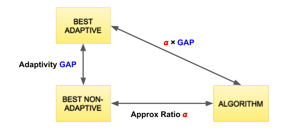 Figure 1
Peer Reviews
No public reviews on file for this paper yet. If you reviewed it on a platform where reviews are public (OpenReview, ICLR, NeurIPS, ICML), you can paste yours below so the community can read it here.
Videos
No videos yet. Explain this paper in a talk, walkthrough, or lecture? Add one.
(Near) Optimal Adaptivity Gaps for
Stochastic Multi-Value Probing
Domagoj Bradac
([email protected]) Department of Mathematics, Faculty of Science, University of Zagreb.
Sahil Singla
([email protected]) Department of Computer Science, Princeton University. Most of this work was done when the author was a graduate student at Carnegie Mellon University.
Goran Zuzic
([email protected]) Computer Science Department, Carnegie Mellon University.
Abstract
Consider a kidney-exchange application where we want to find a max-matching in a random graph. To find whether an edge exists, we need to perform an expensive test, in which case the edge appears independently with a known probability . Given a budget on the total cost of the tests, our goal is to find a testing strategy that maximizes the expected maximum matching size.
The above application is an example of the stochastic probing problem. In general the optimal stochastic probing strategy is difficult to find because it is adaptive—decides on the next edge to probe based on the outcomes of the probed edges. An alternate approach is to show the adaptivity gap is small, i.e., the best non-adaptive strategy always has a value close to the best adaptive strategy. This allows us to focus on designing non-adaptive strategies that are much simpler. Previous works, however, have focused on Bernoulli random variables that can only capture whether an edge appears or not. In this work we introduce a multi-value stochastic probing problem, which can also model situations where the weight of an edge has a probability distribution over multiple values.
Our main technical contribution is to obtain (near) optimal bounds for the (worst-case) adaptivity gaps for multi-value stochastic probing over prefix-closed constraints. For a monotone submodular function, we show the adaptivity gap is at most and provide a matching lower bound. For a weighted rank function of a -extendible system (a generalization of intersection of matroids), we show the adaptivity gap is between and . None of these results were known even in the Bernoulli case where both our upper and lower bounds also apply, thereby resolving an open question of Gupta et al. [GNS17].
1 Introduction
Consider a kidney-exchange application where we want to find a maximum matching in a random graph. To find whether an edge exists, we need to perform an expensive test, in which case the edge appears independently with a known probability . Given a budget on the total cost of the tests, our goal is to design a testing strategy that maximizes the expected size of the found matching.
The above application can be modeled as a constrained stochastic probing problem [ANS08, GN13, ASW14, GNS16, GNS17]. In this setting, we are given a universe of elements (e.g., the set of all possible edges), each with an activation probability for (e.g., the probability an edge exists). We define a random set of active elements that contains every independently with probability . A probe at reveals whether or , and we are only allowed to probe certain feasible subsets (e.g., subsets of edges whose tests fit in our budget). Our goal is to design a probing strategy to find a feasible set of elements to maximize , where is some combinatorial function (e.g., the cardinality of the maximum matching). Notice our probing strategy could be adaptive, i.e., we could decide which element to probe next based on the outcomes of already probed elements.
Besides matching [CIK*+*09, BGL*+*12], stochastic probing has applications for stochastic variants of several other combinatorial problems. E.g., it can be used for Bayesian mechanism design problems [GN13], robot path-planning problems [GNS16, GNS17], and stochastic set cover problems that arise in database applications [LPRY08, DHK14]. As observed in these prior works, the optimal strategy for stochastic probing can be represented as a binary decision tree where each node represents an element of : You first probe the root node element, and then depending on whether it is active or inactive, you either move to the right or the left subtree. In general, such an optimal decision tree can be exponentially sized and is hard to describe. We do not even understand how to capture it for very simple functions and constraints (e.g., the function with cardinality constraints [HFX18]).
An alternate approach is to focus on non-adaptive strategies. Such a strategy commits to probing a feasible set in the beginning, irrespective of which of these elements turn out active. A non-adaptive strategy has several benefits: (a) it is easy to represent since we can just store the set , (b) it is easy to find for many classes of functions and constraints (e.g., submodular functions over intersection of matroids [CVZ14]), and (c) it is parallelizable because we do not need feedback. The concern is that the expected value of the optimal non-adaptive strategy might be much smaller than that of the optimal adaptive strategy. This raises the (worst-case instance) adaptivity gap question: What is the maximum ratio between the expected values of the optimal adaptive and the optimal non-adaptive strategies for stochastic probing? If this ratio is small then we can focus on non-adaptive strategies and reap its benefits with only a small loss in value (see Figure 1).
Since for general combinatorial functions or constraints the adaptivity gaps can be made arbitrarily large, we need to consider special classes of functions and constraints. In a surprising result, Gupta et al. prove that for any monotone submodular function and any prefix-closed constraints111Prefix-closed constraints stipulate that any prefix of a feasible probing sequence is also feasible. This class contains any downward-closed/packing constraint., the adaptivity gap is at most [GNS17]. The best known lower bound in this setting, however, is only due to Asadpour et al. [ANS08]. This leaves open the following question:
For stochastic probing, what is the (worst-case) adaptivity gap for monotone submodular functions over prefix-closed constraints?
We show that both the previously known upper bound of and the lower bound of are not tight. Instead, the adaptivity gap is exactly .
One might notice that submodular functions do not capture the max-matching function used to model kidney-exchanges. This motivates us to consider more general combinatorial functions; in particular, we study the weighted rank function of a -extendible system (defined in §2). This class generalizes intersection of -matroids [Mes06], e.g., a -extendible system captures matching in general graphs (unlike intersections of two matroids). Our goal is to bound the adaptivity gap for such functions over arbitrary prefix-closed constraints.
A major drawback of the stochastic probing model is that it only considers Bernoulli random variables. One would ideally allow for more modeling power by permitting the outcome of a probe to be a non-binary value. For example, in the kidney-exchange application, one might desire to summarize an edge probe by the risk involved in performing the match: a value of [math] describes an impossible match, a value of indicates a safe match, and the possibilities in between are represented by intermediate values. Notice that the optimal adaptive strategy is still a decision tree; however, it may no longer be binary.
The main contributions of this paper are (1) a model that extends the binary stochastic probing to the multi-value setting, (2) the exact calculation of the adaptivity gap for stochastic probing of monotone submodular functions (in both the binary and multi-value setting), and (3) a nearly-tight adaptivity gap for stochastic probing of weighted rank functions over -extendible systems.
1.1 Overview of Results
Our conceptual contribution is to present a generalization of the stochastic probing model to stochastic multi-value probing () described in §2. Roughly, the idea is that each element has potential types, and a probe reveals which one of its types it takes. This trivially captures stochastic probing for , where the two types are active and inactive. In general these different types can be used to model different weights of an element, or to even encode different kinds of complementary relationships in the element values.
Although the model is more general than the stochastic probing model, our main technical result in §3 is that for monotone submodular functions the adaptivity gap is bounded by . We also give a matching lower bound which proves this cannot be further reduced. This is despite the fact that the optimal decision tree for may no longer be binary.
Theorem 1.1**.**
The adaptivity gap for where the constraints are prefix-closed and the function is monotone non-negative submodular is exactly .
Since is strictly more general than stochastic probing, Theorem 1.1 also improves the previously known upper bound of for monotone submodular stochastic probing. In fact, our lower bound instance in Theorem 1.1 is Bernoulli. Thus it resolves an open question of [GNS17] of finding the optimal adaptivity gaps for submodular stochastic probing.
Our main technical result in §4 is that the adaptivity gap for weighted rank function of a -extendible system is .
Theorem 1.2**.**
The adaptivity gap for where the constraints are prefix-closed and the function is a weighted rank function of a -extendible system is between and . Moreover, for unweighted rank functions, the adaptivity gap is between and .
Since the weighted rank of function of intersection of -matroids is a -extendible system, Theorem 1.2 implies as a corollary that the adaptivity gaps for this class is at most . This improves the previously best known upper bound for intersection of matroids of due to Gupta et al. [GNS16]. We also give an -lower bound in this setting.
1.2 Techniques and Challenges
In this section we outline our main techniques and challenges for adaptivity gaps.
Submodular Functions: To prove a small adaptivity gap, we need to show existence of a “good” non-adaptive solution. A priori it is not clear how to construct such a solution, e.g., LP based approaches do not extend beyond matroid constraints because of large integrality gaps. Since we only need to show existence, we can assume the optimal (exponential sized) decision tree is known. A crucial idea of [GNS16] is to perform a random walk on this optimal decision tree (with probabilities given by the tree) and probing elements on the sampled root-leaf path. In other words, consider a non-adaptive strategy that randomly chooses a root-leaf path in the decision tree with the same probability as the optimal adaptive strategy. While this idea is natural in hindsight, its analysis for the non-adaptive strategy has been challenging.
In [GNS16], the authors use Freedman’s inequality—linear functions are “well-concentrated” for a martingale—to argue that simple submodular functions are well-concentrated. This step requires massive union bounds over a polynomial number of linear functions, which loses logarithmic factors. To overcome this super-constant loss, in [GNS17] the authors use an inductive approach and induct over subtrees where in each step a stem—the all-no path—is observed. A “stem lemma” allows them to argue that for every stem the expected value of the non-adaptive algorithm is within a factor to the expected adaptive strategy. Finally, they “stitch” back the stem for induction by using submodularity, overall losing a factor of .
In this work, to prove the improved adaptivity gap of in Theorem 1.1, our insight is to modify the above induction to observe a single node at each step (instead of a stem as in [GNS17]). While we still induct over subtrees, this allows us to avoid any additional loss due to the stitching step. This induction turns out to be nontrivial because the adaptive and non-adaptive strategies can observe different types of the root element. In other words, although the non-adaptive random walk strategy follows the distribution of root-leaf paths of the adaptive strategy, it has to independently re-sample (re-probe) all the nodes on the chosen path. This hinders a direct application of induction as the marginal values in the subtrees change between the two strategies. We remedy this issue using two main ideas. First, we compare the non-adaptive strategy to a “super-strategy” that can choose from both the elements chosen by the adaptive and the non-adaptive strategies. (This is also the intuition for the gap of since the “super-strategy” has two chances to sample an element.) Second, the non-adaptive strategy forfeits any potential future value that the adaptive strategy gained at the root but the non-adaptive missed due to re-sampling. (This can be done by contracting the element sampled by the adaptive strategy without receiving its value.) Notice that both these steps are pessimistic and hence give a valid upper bound on the adaptivity gap. Together these ideas suffice to match the marginal values in the subtrees and apply induction without the stiching step, yielding an adaptivity gap of . Our lower bounds in §3.2 show examples where the super-strategy does not have any advantage over the adaptive strategy. Thus the adaptivity gap of is optimal.
Rank Functions: A technical challenge in extending the above inductive approach to -extendible system rank functions is that their marginal values do not belong to the same class. Namely, after contracting an element, the marginal value of a submodular function is submodular but the marginal value of a -extendible system rank function may not even be subadditive. To overcome this, we first focus on unweighted rank functions. Instead of directly comparing the non-adaptive strategy to the adaptive strategy, our insight is to compare it to a greedy procedure. We show that this greedy procedure is a -approximation to the adaptive strategy. Moreover, we show it has a notion of a marginal value. This allows us to compare the non-adaptive strategy to the greedy procedure in a similar way as for submodular functions, by losing another factor of . Our lower bound in §4.3 shows that the factor loss in comparing to a greedy procedure is unavoidable, thereby making our analysis tight up to constants.
Finally, the challenge in proving Theorem 1.2 for weighted -extendible system rank functions is that the greedy procedure only guarantees a -approximation if we go in the order of decreasing weights. Instead, our adaptivity gap proofs only work when we are greedy in the root-to-leaf path order. One way around this is to partition the elements into exponentially weighted classes (e.g., ) and apply the unweighted argument to the most valuable class. Unfortunately, this loses an factor. To obtain bounds independent of the universe size , our insight is that picking an element in a class “removes” at most elements from a lower weight class. We can therefore improve the factor loss to a by increasing the gap between successive classes to . To achieve this we further combine consecutive classes into a “super-class” (bucket). It is an interesting open question to find if this loss is essential in going from unweighted to weighted -extendible system rank functions.
1.3 Further Related Work
The adaptivity gap of stochastic packing problems has seen much interest; see, e.g., for knapsack [DGV04, BGK11, Ma14], packing integer programs [DGV05, CIK*+*09, BGL*+*12], budgeted multi-armed bandits [GM07, GKMR11, LY13, Ma14], and orienteering [GM09, GKNR12, BN14]. All except the orienteering results rely on having relaxations that capture the constraints of the problem via linear constraints. For stochastic monotone submodular functions where the probing constraints are given by matroids, Asadpour et al. [AN16] bounded the adaptivity gap by ; Hellerstein et al. [HKL15] bound it by , where is the smallest probability of some set being materialized. Other relevant papers are [LPRY08, DHK14].
The work of Chen et al. [CIK*+*09] (see also [Ada11, BGL*+*12, BCN*+*15, AGM15]) sought to maximize the size of a matching subject to -matching constraints; this was motivated by applications to online dating and kidney exchange. See also [RSÜ05, AR12] for pointers to other work on kidney exchange problems. The work of [GN13] abstracted out the general problem of maximizing a function (in their case, the rank function of the intersection of matroids or knapsacks) subject to probing constraints (again, intersection of matroids and knapsacks). This was improved and generalized by Adamczyk et al. [ASW14] to submodular objectives. All these results use LPs or geometric relaxations, and do not extend to arbitrary packing constraints due to large integrality gaps of the relaxations.
2 Stochastic Multi-Value Probing Model
In this section we formally define our stochastic multi-value probing () model using the idea of combinatorial valuation over independent elements. We also discuss some preliminaries.
2.1 Combinatorial Valuation over Independent Elements
The multi-value paradigm is based on the notion of type, which represents different “values” an element can take. This leads to combinatorial valuations over independent elements where each element independently takes its type. Similar notions have been defined before; e.g., see [RS17] and references therein.
Definition 2.1** (Combinatorial valuation over independent elements).**
Consider a finite universe of elements and size . Each element obtains exactly one type from a finite set according to a given probability distribution over . These types are assigned independently across different elements, i.e., the random vector of types is drawn from the product distribution . Given a combinatorial function for , the valuation of a set is
[TABLE]
where we define \mathbf{X}_{S}\stackrel{{\scriptstyle\mathrm{def}}}{{=}}\big{\{}\mathbf{X}_{e}\mid e\in S\big{\}} to simplify notation.
For example, in the Bernoulli case studied in the stochastic probing literature, each element has two types: active and inactive, the distributions are Bernoulli, and the valuation function . Another example is the multi-value max-weight matching problem described in the introduction. Here different types of an element (edge) correspond to its different weights and is the max-weight matching in the induced subgraph on .
In this work we always assume the combinatorial function satisfies and is monotone, i.e., for all . We also assume it belongs to one of the following classes.
- •
subadditive if for all .
- •
submodular if for all . For , the contraction
[TABLE]
of a monotone submodular function is also monotone submodular.
- •
weighted rank function of a family if where is a linear function with non-negative weights. When is the all ones vector (i.e., ), we call it the unweighted rank function of .
In particular, we work with rank functions of two special families . Subsets in the family are called independent subsets. A family forms a
- •
matroid if for every with there exists such that .
- •
-extendible system if for every and where , we have that there is a set such that and .
This latter family is important because it generalizes the family of intersection of matroids, e.g., a -extendible systems captures general graph matchings (see [CCPV11] for further discussion).
2.2 Adaptive Strategies and
Roughly, the goal of an problem is to maximize a combinatorial function over independent elements under some “feasibility constraints”. We define a probe of an element to be an operation that reveals its random type . A probing sequence is an ordered sequence of probes on some elements.
The problem only allows a family of probing sequences , which are called feasible. We assume minimal properties from this family. Specifically, it is prefix-closed, i.e., for every sequence in , each of its prefix is also in . This prefix-closed family is powerful because it generalizes any downward-closed family (i.e., for all and we have ) and can also capture precedence constraints.
We now define an adaptive strategy which constitutes a feasible solution for . The nodes in this tree correspond to probes of elements
Definition 2.2** (Adaptive strategy ).**
It is a rooted decision tree where each non-leaf node is labeled with an element and has arcs to child nodes. Each arc is uniquely labeled with a type . Whenever we encounter a node labeled , the adaptive strategy probes and proceeds to the subtree corresponding to the arc labeled . The strategy terminates on reaching a leaf and receives a value of , where is the set of probed elements by strategy for type vector . The objective is the expected valuation, which we denote by
[TABLE]
Notice, since is monotone, a strategy never gains value by removing a probed element. We say a strategy is feasible for if every root-leaf path belongs to . We now formally define an problem.
Definition 2.3** ( problem ).**
Given a prefix-closed family of probing constraints and a combinatorial valuation over independent elements, an problem is to find a feasible adaptive strategy to maximize the expected valuation .
2.3 Non-Adaptive Strategies and Adaptivity Gaps
A strategy to solve an problem can benefit from adjusting its probing sequence based on the outcomes of the already probed elements. For instance, in the kidney-exchange example if one finds an edge incident to a vertex , one may choose not to probe any other edges incident to . On the other hand, a strategy that always decides the next probe independent of the outcomes of the probed elements is called non-adaptive. Our goal is to study the largest ratio between adaptive and non-adaptive strategies.
Definition 2.4** (Adaptivity gap for ).**
Let be a class of SMP problems (e.g., monotone submodular functions over prefix-closed constraints). Define the adaptivity gap as the largest (worst-case instance) ratio of the optimal adaptive and optimal non-adaptive strategies for a problem , i.e.,
[TABLE]
Notice that in the denominator does not depend on .
The adaptivity gap for a general combinatorial function is unbounded [GNS16]. In this work we focus on monotone submodular functions and (weighted) rank functions of a -extendible system. We bound adaptivity gaps by analyzing the following natural random walk non-adaptive strategy.
Definition 2.5** (Random walk non-adaptive strategy).**
For any given adaptive strategy , there is a corresponding non-adaptive strategy that (virtually) draws a sample from the product distribution and traverses along the root-leaf path for (i.e., when at a node labeled , traverse the unique arc labeled ). Let be the random set of elements probed by such a root-leaf path. The true (non-virtual) types of elements correspond to the vector of outcomes . Here and are i.i.d. r.v.s. The random walk non-adaptive strategy probes according to the above distribution and receives the valuation
[TABLE]
3 Adaptivity Gaps for a Monotone Submodular
Function
In this section we prove our first main result, the optimal adaptivity gap for submodular functions. In §3.1 we prove the upper bound and in §3.2 we prove the lower bound of Theorem 1.1. See 1.1
3.1 Upper Bound of
Our non-adaptive strategy samples a random root-leaf path using the optimal adaptive strategy tree (2.5). In other words, it performs a “dry-run” of a random walk along the tree without probing anything. In the end it queries all the elements on this random root-leaf path. We argue that its expected value is at least half of the adaptive strategy. We encourage the reader to follow the proof idea outlined in §1.2 since algebra can conceal the main ideas.
Proof of the upper bound in Theorem 1.1.
We induct over the depth of the tree , i.e., for any monotone submodular function and tree of depth at most , we have
[TABLE]
The base case for is trivially true because the tree is a single node. For induction, let be the root node of the optimal decision tree . Denote by the (random) type of element when probed by the adaptive strategy (and also the virtual type of the non-adaptive strategy), while be the (random) true type when probed by the non-adaptive strategy. Also, let denote the subtree the adaptive strategy goes to when the root element is in type and let be the contraction from Eq. (1). This implies
[TABLE]
Now using submodularity and monotonicity of , we bound the adaptive strategy
[TABLE]
where the last inequality uses that every monotone submodular function is subadditive. Notice that and are i.i.d. variables. This along with linearity of expectation implies
[TABLE]
Next, we lower bound the expected value of the non-adaptive strategy from Eq. (4). We use monotonicity of to get
[TABLE]
Since is also a monotone submodular function over independent elements and is an adaptive strategy tree of depth at most , by induction hypothesis
[TABLE]
Combining this with Eq. (5) and Eq. (6), we get
[TABLE]
which finishes the proof of the upper bound by induction. ∎
3.2 Lower Bound of
In this section we show a monotone non-negative submodular function and a prefix-closed set of constraints where the adaptivity gap for stochastic probing is arbitrarily close to . Combined with §3.1, this proves Theorem 1.1 that the optimal adaptivity gap is exactly .
The proof below uses a stochastic probing instance on an infinite universe. Since submodular functions are defined only on finite sets, the proof below is informal. We do this to explain our main ideas and defer the formal proof to Appendix A.
Informal proof of the lower bound in Theorem 1.1.
Our example is on a universe where every element is independently active with probability for some .
Example:
We define our submodular objective to be the weighted rank function of a partition matroid that selects at most one element from each part. The elements are partitioned according to their first label—for every the set is a part of the partition matroid with weight . In other words, for any set let be the (unique) set of first labels, then
[TABLE]
Note that this series always converges so is well defined.
To define our prefix-closed constraints, we consider an infinite directed acyclic graph where every element is identified with a single node in the graph. Every node/element has exactly two outgoing edges: towards and towards . We denote as the elements on column . The probing constraint is that a sequence of elements can be probed if and only if it corresponds to a directed path starting at . See Figure 2 for an illustration.
Analysis:
We first give an adaptive strategy with value (in Eq. (7)) and later argue that every non-adaptive strategy has value at most (in Eq. (8)); thereby, proving this theorem. Although, the probing constraint allows for infinite strategies, and in a different setting it would not be clear how to define their expected values, since is monotone we include every active element in the solution. So the expected value of an infinite strategy can be defined as the limit of strategies that only probe a finite number of elements. The finite lower bound example in Appendix A is constructed by reducing so that the resulting strategies are close to this limit.
Our adaptive strategy starts with probing element . It is defined recursively: after probing , the next element to probe is either if is found active, or otherwise. In other words, it probes elements on a column until it finds one active, and then probes another column.
Let denote the expected additional value our above adaptive strategy if the next probed element is and let denote the expected value of the entire strategy. Note that does not depend on the set of elements found active before probing (i.e., the elements where ). Furthermore, the subgraph reachable from is similar to the entire graph on in the sense that one can relabel the elements in the subgraph to match the entire graph exactly, the only difference being that the value of any subset is multiplied by a factor of . Therefore, we have
[TABLE]
Now, summing over the number of inactive elements on column [math], we get
[TABLE]
which uses . Solving this equation yields the result:
[TABLE]
Similarly, let denote the expected additional value of the optimal non-adaptive strategy if the next probed element is , and let denote the expected value of the optimal non-adaptive strategy. By the same argument as , we have
[TABLE]
Let denote the number of elements the optimal non-adaptive strategy probes on column [math]. We get
[TABLE]
which uses . This implies
[TABLE]
Combining Eq. (7) and Eq. (8), we get an adaptivity gap arbitrarily close to for . ∎
4 Adaptivity Gaps for a Weighted Rank Function of a -Extendible
System
For a downward-closed family , recollect that we define its rank function to be the largest cardinality subset in , i.e., . In this section we prove our results on the adaptivity gaps of a weighted rank function of a -extendible system. See 1.2
In §4.1 we prove the upper bound for unweighted -extendible systems, and in §4.2 we give a reduction from weighted to unweighted -extendible systems that loses a factor in the adaptivity gap. Our lower bound is presented in §4.3.
To simplify our proofs, we define an element as a loop in if . Furthermore, given a non-loop element , we define the contraction as , i.e., the family of subsets that contain but with removed. We also need the following property of -extendible systems, which intuitively means a set hurts at most from another set . We include the proof for completeness in Appendix B.
Fact 4.1**.**
Let be a -extendible system. For every and where , there exists a set such that and .
4.1 Upper Bound of for an Unweighted -Extendible System
Let denote the optimal adaptive strategy for maximizing the rank function of a given -extendible system . We prove the following unweighted upper bound of Theorem 1.2.
Theorem 4.2**.**
The adaptivity gap for where the constraints are prefix-closed and the function is an unweighted rank function of a -extendible system is at most .
We use the random walk strategy to convert the adaptive strategy into a non-adaptive strategy. To analyze our algorithm, we define a natural greedy procedure to select a subset of that is also in . First, consider elements of in an arbitrary order (which can even be determined on the fly). If the currently considered element is a non-loop, it gets contracted in ; otherwise it gets ignored. Any such computed set is in and the final output, the number of contracted elements, is denoted by . We first show that for -extendible systems such a greedy procedure produces a -approximation to the largest subset in . A similar statement has been proven by Mestre [Mes06].
Lemma 4.3**.**
Let be a rank function of a -extendible system . Fix any subset and consider the output of the greedy procedure with an arbitrary ordering of . We have that . Even more, for any we have that .
Proof.
Let be the set picked by . Notice that is a maximal set in (need not be maximum). On the other hand, let be the set picked by , i.e., the maximum set in on . Our goal is to prove .
Let , note that and , hence by 4.1 there is a with such that . However, since is a maximal set and we know that and hence . ∎
Given the above properties of a -extendible system, we can now prove Theorem 4.2.
Proof of Theorem 4.2.
Let and denote the element types for the adaptive and the non-adaptive algorithms, respectively. The adaptive strategy on the optimal decision tree gets value , where is the set of probed elements by strategy for type vector . We compare this value to a greedy strategy in which
- (a)
we consider the elements of in root-to-leaf order in which they appear on the tree and 2. (b)
for any we first consider (the true type) before (the virtual type) in the greedy order.
Note by Lemma 4.3 we have
[TABLE]
By induction on the subtrees, below we prove
[TABLE]
This finishes the proof of Theorem 4.2 because the optimal non-adaptive algorithm has value at least
[TABLE]
To prove the missing Eq. (9), we induct on the height of the tree and being any downward-closed family. For consistency, we define the notation of to denote the value of the above greedy strategy when run on with a rank function . Thus, . Suppose is the label of the root of . Denote by the (random) type of element when probed by the adaptive strategy (which is also the virtual type of the non-adaptive strategy), and denote the (random) true type when probed by the non-adaptive strategy. Also, let denote the subtree the adaptive strategy goes to when the root is in state . We have
[TABLE]
where by we mean the rank function of after we first contract if it a non-loop, and then contract if it is still a non-loop. Now subadditivity of gives
[TABLE]
where the last equality uses linearity of expectation as and are identically distributed.
Next, we lower bound the value of our non-adaptive algorithm. Although it takes a random root-leaf path and decides the set of elements to retain in the end, we lower bound its value by an online algorithm that greedily selects (unless it is a loop), however, always also contracts if it is a non-loop. This gives,
[TABLE]
Since is also a rank function of a downward-closed system and is an adaptive strategy, by induction hypothesis we have
[TABLE]
Combining this with Eq. (10) and Eq. (11), we get
[TABLE]
which proves Eq. (9) by induction. ∎
4.2 Reducing Weighted to Unweighted -Extendible System by Losing
We show how to extend the adaptivity gap result for an unweighted -extendible system to a weighted -extendible system by losing an factor.
Theorem 4.4**.**
For over prefix-closed constraints, the adaptivity gap for a weighted rank function of a -extendible system is at most .
Proof.
Given a weighted rank function of a -extendible system over a set of types , we define for to be an unweighted rank function of the -extendible system ; however, the new weights are changed such that only the types with original weights in participate with new weight of , while the other elements have a new weight of [math]. Note that this partitions the set of types into pairwise disjoint classes. Notice, we have
[TABLE]
where denotes the expected value of an adaptive strategy given by the common decision tree with respect to the rank function .
Now, since is an unweighted -extendible system problem, we know that a random root-leaf path returns a solution with expected value
[TABLE]
In the following lemma, we show that these non-adaptive solutions for can be combined to obtain a feasible and “high-value” non-adaptive solution for .
Lemma 4.5**.**
The random-walk non-adaptive algorithm has expected value
[TABLE]
Before proving Lemma 4.5, we finish the proof of Theorem 4.4 by combining it with Eq. (13) and Eq. (12):
[TABLE]
Informally, in the proof of Lemma 4.5 we combine the unweighted solutions of by running a “greedy-optimal” algorithm from the higher weight to the smaller weight classes and fixing the types chosen in earlier classes. Unfortunately, in general such an approach loses an extra factor in the approximation. To fix this, our second idea is to increase the weight gap between successive classes. We achieve this by combining consecutive classes into a bucket, where in each bucket we focus on the class with the largest non-adaptive value. Because of boundary issues, we only take either odd or even buckets.
Proof of Lemma 4.5.
Let denote the indices of the smallest and the highest weight classes. We define buckets consisting of consecutive classes, where bucket consists of classes . For each , let
[TABLE]
Since each bucket has size , this implies
[TABLE]
Without loss of generality we can assume the odd indices satisfy
[TABLE]
Otherwise, use the same argument for even indices. Combining the last two equations, we get
[TABLE]
We now claim that a greedy-optimal algorithm has a large value: It goes over classes in decreasing order of (odd) buckets, but it always selects the maximum independent set (instead of selecting a maximal greedy set) in the current class given its choices in the previous. This algorithm is, therefore, a combination of greedy and optimal algorithms.
Claim 4.6**.**
Consider an algorithm that goes over the odd numbered buckets in decreasing order of weights and selects the maximum set from class in bucket such that the resulting set is still feasible in . (After a set in a class is selected, it gets fixed for all smaller choices.) The finally chosen set has value at least
[TABLE]
Proof.
The intuition is that for a -extendible system by 4.1 any selected member can “hurt” at most members from lower buckets. Since we only consider odd numbered buckets, two types in different buckets differ in their weights by at least a factor of . Thus, losing types of lower weight should not significantly impact the value.
Let be the random variable denoting the leaf reached by the random walk on the decision tree , and let be the random set of elements seen by the random-walk non-adaptive strategy on this path. Furthermore, let denote the set of elements picked by the non-adaptive strategy with respect to , let be the set of elements picked by our greedy-optimal non-adaptive strategy from bucket , and let denote . In other words, is the greedy-optimal solution up to bucket number and is the maximum subset of such that . Note that , and are random variables depending on and .
Using 4.1 on the -extendible system with the preconditions and , there exists a set with such that . Hence, we have
[TABLE]
Multiplying by and summing over all odd gives
[TABLE]
Now, since every bucket contains classes, where two successive class weights differ by a factor of , we know
[TABLE]
Combining this with Eq. (4.2) gives
[TABLE]
where the last inequality uses
[TABLE]
After rearranging,
[TABLE]
Notice that by definition of a class, each type in class has weight at least . Using this fact and taking expectation over and , we get
[TABLE]
which finishes the proof of 4.6. ∎
Using 4.6, we have
[TABLE]
which combined when with Eq. (14) proves Lemma 4.5. ∎
4.3 Lower Bounds
We present two very similar lower bound examples: one where the adaptivity gap is for a rank function of an unweighted -extendible system and another where the adaptivity gap is for a rank function of an intersection of matroids. A related example was also shown in [GNS17].
Example:
For generality we work in the Bernoulli setting where each element in is either active or inactive. Consider a perfect -ary tree of depth whose edges correspond to the ground set . Each edge is active with probability . For any leaf , let denote the unique path from the root to . The objective value on any set is the maximum number of edges in the set on the same root-leaf path, i.e., for any ,
[TABLE]
The feasibility constraints are such that a set of edges can be probed if and only if there exists some root-leaf path such that every probed edge has at least one endpoint on Note that this implies that a maximum of edges can be probed.
Analysis:
Let the adaptive strategy be the following: probe all edges incident to the root. If any of them is active, start probing the edges directly below the active edge, otherwise below the first edge. Continue recursively until a leaf is reached. On every level, the adaptive strategy has probability of finding an active edge. Therefore, the expected value of the adaptive strategy is
For any non-adaptive strategy, the feasibility constraints imply there exists a root-leaf path such that all probed edges have an endpoint on it. Suppose all edges incident to are probed. The non-adaptive strategy can get value at most from the edges not on and in expectation at most from the edges on So, the non-adaptive strategy has an expected value of at most
Lower Bound of for an unweighted -extendible system
Consider the example described above and set and . The function is trivially a rank function of a -extendible system because the rank of the system is , i.e., . The adaptive strategy has an expected value
[TABLE]
whereas any non-adaptive strategy has an expected value at most This gives an adaptivity gap of .
Lower Bound of for an unweighted
intersection of matroids
In this section we show how to model the above example as an intersection of matroids, yielding an adaptivity gap of for an intersection of matroids. Consider the example described above and set and . The adaptive strategy has an expected value of
[TABLE]
and the non-adaptive strategy gets at most in expectation; so the adaptivity gap is .
All that remains to show is that can be represented as an intersection of simple partition matroids. We use the term simple partition matroid for a matroid that partitions the into multiple parts and a set is independent if it contains at most one element in every part.
Suppose that is prime and label each node with a list as follows: the root’s label is an empty list . Let denote the element of the list and a list equal to with appended to it. All the other nodes are labeled recursively: let be a node with children . Define . Hence, is an ancestor of if and only if is a prefix of , and otherwise for some .
Let denote the edge/element between and its parent. We define partition matroids for and . Each consists of big partitions indexed from [math] to , and all other partitions contain only a single element. Let
[TABLE]
For a node on depth , element is in the big partition of . For a node on depth , is the only element in its partition in .
We claim that is the rank function of , which is an intersection of matroids. Since is an intersection of simple partition matroids, if and only if for every . Now consider two nodes such that . This means for some and , which is equivalent to
[TABLE]
Since is prime, this holds for some if and only if (for ) or for any . That is, if and only if and are not ancestors of one another, which completes the proof.
Acknowledgments. We thank Anupam Gupta for useful discussions. The second author was supported in part by NSF awards CCF-1319811, CCF-1536002, and CCF-1617790. The third author was supported in part by CCF-1527110, CCF-1618280 and NSF CAREER award CCF-1750808.
Appendix A Adaptivity Gap Lower Bound of for Submodular Functions
Proof.
As mentioned, the finite lower bound example is constructed by reducing the infinite example given in Section 3.2. However, this reduction loses the nice similarity properties of the graph so much more calculation is required in order to bound the strategies.
Let and be the smallest integer such that . The ground set is the result of removing elements where , that is where each node is active with probability . The probing constraint and the objective function are naturally reduced to this set: a sequence of elements can be probed if they correspond to a (finite) path starting at in the given graph, and where is the set of (unique) first labels which now finite. Similarly as before, we will denote as the vertices on the column .
We first show that any non-adaptive strategy has expectation at most 1. Let denote the additional expected value of the optimal non-adaptive strategy if the next probed element is . We will inductively prove , which is sufficient for our claim. For the base case , the inequality clearly holds since . For let be the second label of the last vertex probed on the column .
[TABLE]
This completes the induction and proves that non-adaptive strategies get at most .
Finally, we show that there exists an adaptive strategy with expected value at least for sufficiently small . This finalizes the proof since it implies a gap of by taking . The strategy is naturally reduced: first probe and after probing some terminate if , otherwise probe if is active and if not. Let denote the expected value this strategy gets when the next probed element is , for . For convenience, define for all .
We prove by induction that , which is sufficient to finalize the proof since then . For large enough that , the inequality clearly holds and presents our base case. Otherwise, . Let be the second label of the last vertex probed on the column and let denote the set of active elements.
[TABLE]
Using the induction hypothesis, we get
[TABLE]
After dropping some positive summands and using and , we get
[TABLE]
It is sufficient to prove
[TABLE]
Multiplying by , we get an equivalent statement to prove:
[TABLE]
Finally, using and expanding out, we note that the left-hand side is , while the right-hand side is . Therefore, the inequality holds for sufficiently small . This concludes the proof. ∎
Appendix B Proof of the -Extendible Property for Set Extension
See 4.1
Proof.
Enumerate the elements where and denote by for . Initialize and consider the following procedure to construct that satisfies the invariants , and .
In the step we have that by downward-closeness and by the induction hypothesis. Hence by -extendibility we can find with and where . Set and note that . Furthermore, already deduced that and finally since . We satisfied all stipulations of the induction, hence we report as the solution. ∎
The reference list from the paper itself. Each links out to its DOI / PubMed record.
- 1[Ada 11] Marek Adamczyk. Improved analysis of the greedy algorithm for stochastic matching. Inf. Process. Lett. , 111(15):731–737, 2011.
- 2[AGM 15] Marek Adamczyk, Fabrizio Grandoni, and Joydeep Mukherjee. Improved approximation algorithms for stochastic matching. In Algorithms-ESA 2015 , pages 1–12. Springer, 2015.
- 3[AN 16] Arash Asadpour and Hamid Nazerzadeh. Maximizing stochastic monotone submodular functions. Management Science , 62(8):2374–2391, 2016.
- 4[ANS 08] Arash Asadpour, Hamid Nazerzadeh, and Amin Saberi. Stochastic submodular maximization. In International Workshop on Internet and Network Economics , pages 477–489. Springer, 2008. Full version appears as [ AN 16 ] .
- 5[AR 12] Itai Ashlagi and Alvin E. Roth. New challenges in multihospital kidney exchange. American Economic Review , 102(3):354–59, 2012.
- 6[ASW 14] Marek Adamczyk, Maxim Sviridenko, and Justin Ward. Submodular stochastic probing on matroids. In STACS , pages 29–40, 2014.
- 7[BCN + 15] Alok Baveja, Amit Chavan, Andrei Nikiforov, Aravind Srinivasan, and Pan Xu. Improved bounds in stochastic matching and optimization. In Approximation, Randomization, and Combinatorial Optimization. Algorithms and Techniques, APPROX/RANDOM 2015, August 24-26, 2015, Princeton, NJ, USA , pages 124–134, 2015.
- 8[BGK 11] Anand Bhalgat, Ashish Goel, and Sanjeev Khanna. Improved approximation results for stochastic knapsack problems. In SODA , pages 1647–1665, 2011.