A Sieve-SMM Estimator for Dynamic Models
Jean-Jacques Forneron

TL;DR
This paper introduces a flexible Sieve-SMM estimator for nonlinear dynamic models that accurately estimates parameters and shock distributions without requiring parametric assumptions, improving robustness against misspecification.
Contribution
It develops a novel Sieve-SMM approach that approximates shock distributions with a Gaussian and tails mixture sieve, extending asymptotic theory to complex models with latent variables.
Findings
Estimator achieves consistency, rate of convergence, and asymptotic normality.
Application reveals significant reduction in estimated relative risk-aversion.
Method improves robustness in asset pricing models.
Abstract
This paper proposes a Sieve Simulated Method of Moments (Sieve-SMM) estimator for the parameters and the distribution of the shocks in nonlinear dynamic models where the likelihood and the moments are not tractable. An important concern with SMM, which matches sample with simulated moments, is that a parametric distribution is required. However, economic quantities that depend on this distribution, such as welfare and asset-prices, can be sensitive to misspecification. The Sieve-SMM estimator addresses this issue by flexibly approximating the distribution of the shocks with a Gaussian and tails mixture sieve. The asymptotic framework provides consistency, rate of convergence and asymptotic normality results, extending existing results to a new framework with more general dynamics and latent variables. An application to asset pricing in a production economy shows a large decline in the…
Click any figure to enlarge with its caption.
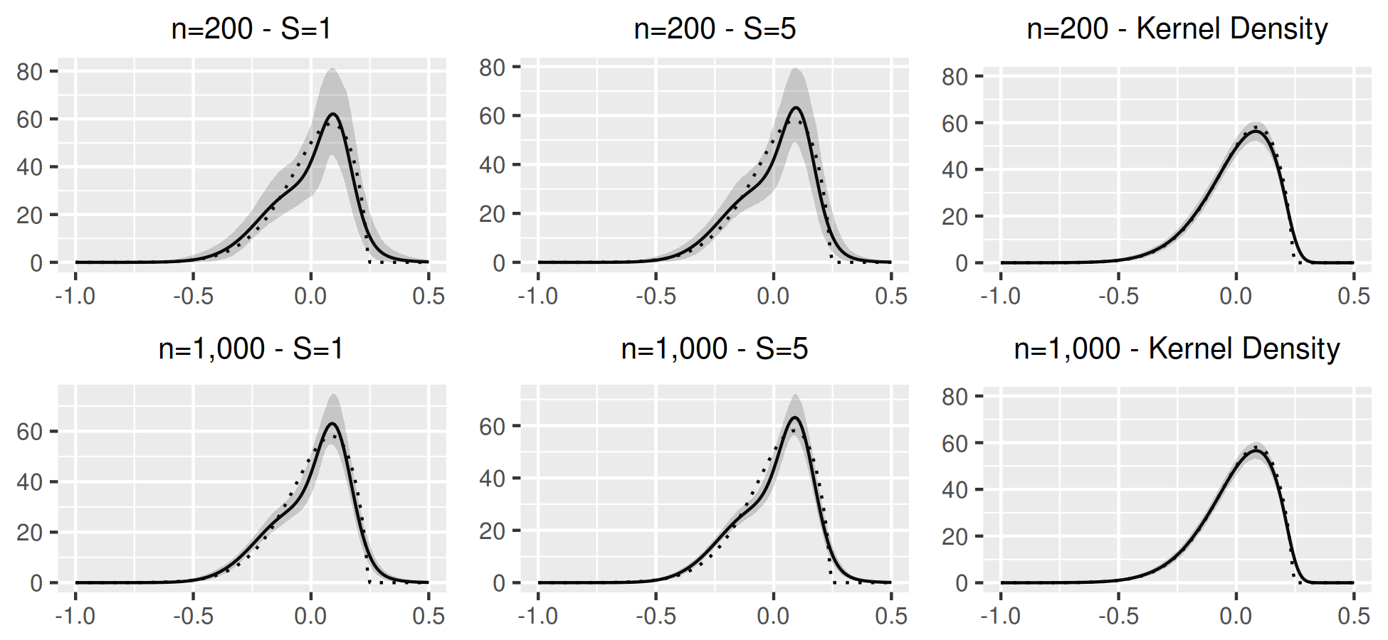 Figure 1
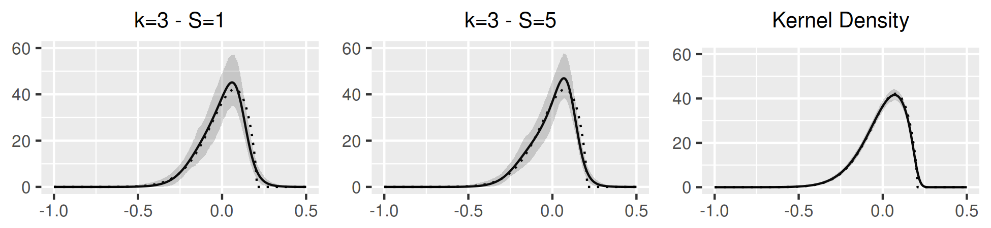 Figure 2
 Figure 3
 Figure 4
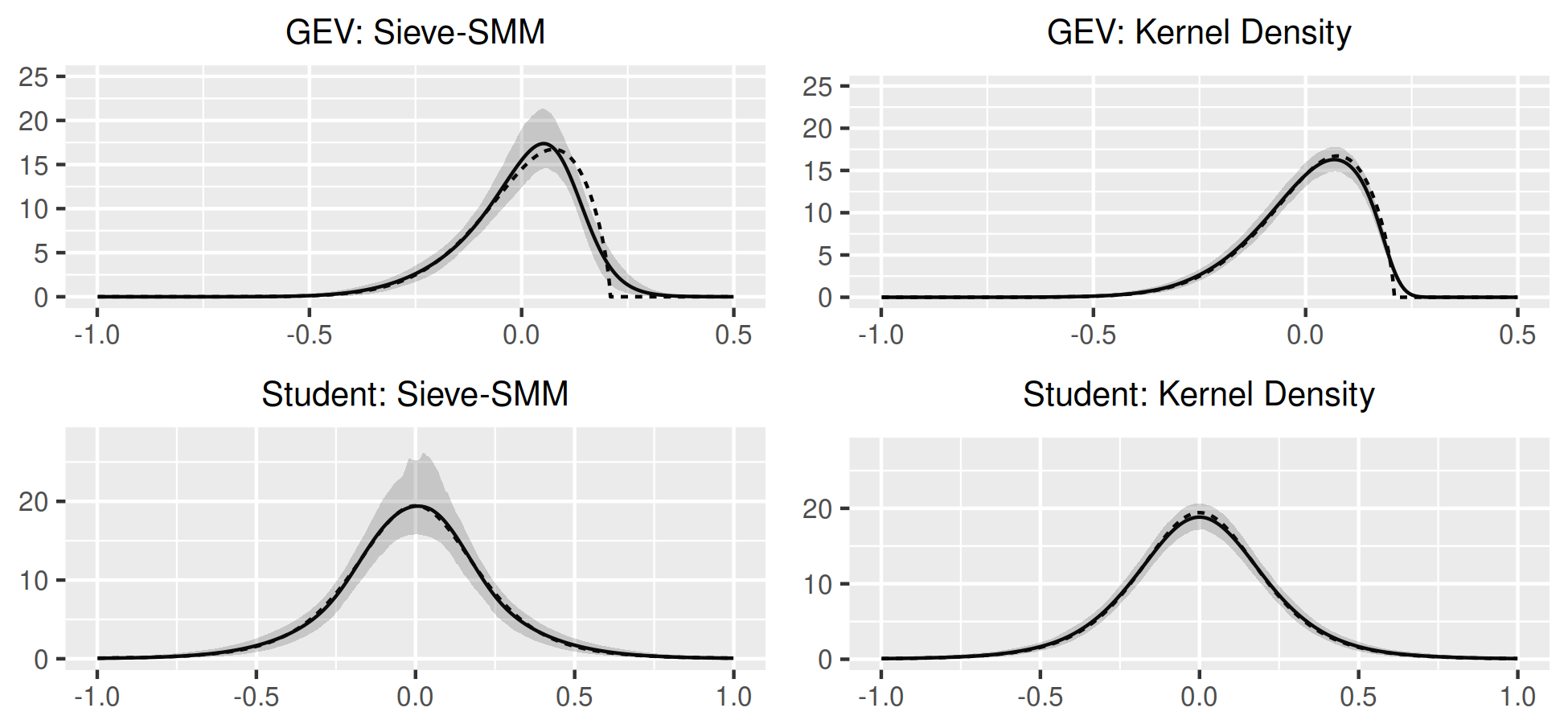 Figure 5
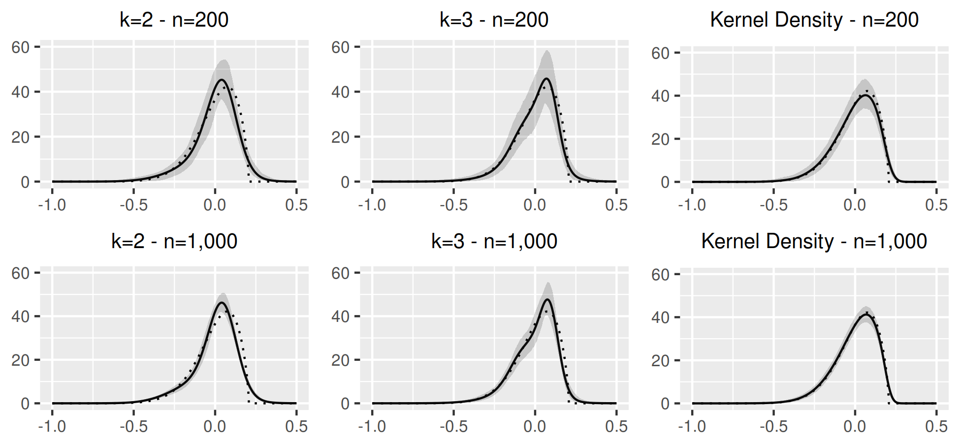 Figure 6
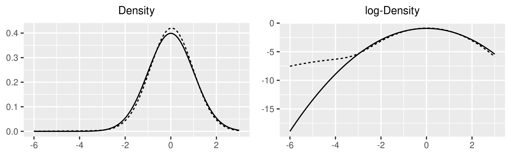 Figure 7
| Sieve-SMM | Bayesian | GMM | ||||||
| 2 | 3 | 2 | 3 | - | ||||
| 1 | 5 | 1 | 5 | - | - | - | ||
| AR(1) | bias | -0.014 | -0.010 | -0.017 | -0.016 | -0.011 | -0.010 | -0.015 |
| std | 0.082 | 0.064 | 0.077 | 0.062 | 0.048 | 0.049 | 0.056 | |
| size | 0.044 | 0.033 | 0.026 | 0.018 | 0.051 | 0.054 | 0.019 | |
| SV | bias | -0.003 | -0.006 | -0.002 | -0.006 | - | - | -0.006 |
| std | 0.014 | 0.012 | 0.015 | 0.012 | - | - | 0.027 | |
| size | 0.200 | 0.170 | 0.190 | 0.140 | - | - | 0.060 | |
| 0.994 | 34.629 | 0.145 | 1000.000 | 0.985 | -0.990 | -0.100 | 0.001 | 0.005 | 3.58 | |
| (0.001) | (15.373) | (0.007) | (3465.036) | (0.004) | (0.051) | (0.012) | (0.011) | (0.003) | ||
| 0.972 | 20.153 | 0.192 | 50.526 | 0.766 | -0.152 | -0.127 | -0.015 | 0.007 | 2.73 | |
| (0.014) | (4.939) | (0.010) | (19.425) | (0.036) | (0.049) | (0.014) | (0.014) | (0.002) | ||
| 0.988 | 12.754 | 0.189 | 54.559 | 0.774 | -0.059 | -0.099 | -0.010 | 0.007 | 2.70 | |
| (0.007) | (3.339) | (0.011) | (18.263) | (0.029) | (0.046) | (0.015) | (0.014) | (0.002) | ||
| 0.992 | 10.476 | 0.165 | 51.906 | 0.711 | 0.005 | -0.112 | -0.004 | 0.007 | 2.58 | |
| (0.006) | (2.692) | (0.012) | (13.748) | (0.039) | (0.048) | (0.014) | (0.014) | (0.002) | ||
| 0.991 | 11.970 | 0.170 | 66.961 | 0.694 | 0.139 | -0.085 | -0.016 | 0.007 | 2.46 | |
| (0.007) | (3.147) | (0.011) | (24.847) | (0.034) | (0.045) | (0.012) | (0.012) | (0.002) | ||
| lb | 0.965 | 0.5 | 0.05 | 0.01 | 0.2 | -0.99 | -0.25 | -0.25 | 0.005 | - |
| ub | 0.999 | 70 | 110 | 1000 | 0.995 | 0.2 | 0.25 | 0.25 | 0.0085 | - |
| Average Yield | Standard Deviations | Corr(,Yield) | ||||||||||||
|---|---|---|---|---|---|---|---|---|---|---|---|---|---|---|
| Sample | 4.57 | 4.71 | 5.03 | 5.24 | 3.19 | 3.18 | 3.31 | 3.25 | 0.57 | 1.96 | 0.07 | 0.07 | 0.08 | 0.09 |
| Gaussian | 2.80 | 2.87 | 2.99 | 3.05 | 2.44 | 2.35 | 2.31 | 2.26 | 0.53 | 1.66 | -0.25 | -0.25 | -0.25 | -0.25 |
| 3.59 | 3.64 | 3.73 | 3.85 | 1.66 | 1.43 | 1.11 | 0.73 | 0.83 | 1.23 | -0.11 | -0.07 | -0.04 | -0.02 | |
| 3.74 | 3.76 | 3.80 | 3.85 | 1.96 | 1.72 | 1.37 | 0.92 | 0.68 | 1.48 | -0.06 | -0.03 | -0.01 | 0.01 | |
| 3.88 | 3.88 | 3.89 | 3.90 | 1.90 | 1.63 | 1.22 | 0.76 | 0.69 | 1.42 | 0.01 | 0.03 | 0.05 | 0.07 | |
| 3.81 | 3.83 | 3.86 | 3.89 | 1.94 | 1.70 | 1.28 | 0.79 | 0.66 | 1.41 | -0.02 | 0.02 | 0.04 | 0.05 | |
| 5.08 | 5.08 | 5.08 | 5.08 | 1.90 | 1.63 | 1.23 | 0.77 | 0.34 | 2.04 | -0.16 | -0.17 | -0.15 | -0.08 | |
| 95% CI for | 95% CI for | |||||
|---|---|---|---|---|---|---|
| 0.001 | 0.004 | 0.029 | 0.013 | |||
| 0.020 | 0.008 | 0.050 | 0.012 | |||
| 0.018 | 0.006 | 0.079 | 0.021 | |||
| 0.019 | 0.005 | 0.096 | 0.025 | |||
| 0.015 | 0.005 | 0.084 | 0.022 |
| Sieve-SMM | Bayesian | GMM | ||||||
| 2 | 3 | 2 | 3 | - | ||||
| 1 | 5 | 1 | 5 | - | - | - | ||
| AR(1) | bias | -0.023 | -0.025 | -0.030 | -0.032 | -0.024 | -0.023 | -0.031 |
| std | 0.119 | 0.092 | 0.112 | 0.090 | 0.073 | 0.072 | 0.083 | |
| size | 0.047 | 0.037 | 0.033 | 0.027 | 0.055 | 0.053 | 0.016 | |
| S | |||||||||||
|---|---|---|---|---|---|---|---|---|---|---|---|
| 1 | bias | 0.000 | -0.003 | 0.005 | -0.167 | -0.092 | -0.000 | -0.001 | 0.010 | -0.078 | -0.105 |
| std | 0.014 | 0.014 | 0.082 | 0.276 | 0.280 | 0.012 | 0.014 | 0.066 | 0.182 | 0.201 | |
| size | 0.315 | 0.200 | 0.100 | 0.100 | 0.155 | 0.215 | 0.140 | 0.060 | 0.020 | 0.085 | |
| 5 | bias | 0.001 | -0.006 | 0.020 | -0.077 | -0.133 | 0.000 | -0.006 | 0.011 | -0.051 | -0.083 |
| std | 0.009 | 0.012 | 0.062 | 0.216 | 0.210 | 0.008 | 0.012 | 0.053 | 0.126 | 0.138 | |
| size | 0.535 | 0.170 | 0.090 | 0.005 | 0.055 | 0.335 | 0.125 | 0.050 | 0.000 | 0.005 | |
| 20 | bias | 0.000 | -0.005 | 0.012 | -0.041 | -0.116 | -0.000 | -0.005 | 0.008 | -0.020 | -0.066 |
| std | 0.008 | 0.011 | 0.060 | 0.177 | 0.193 | 0.007 | 0.011 | 0.056 | 0.071 | 0.113 | |
| size | 0.505 | 0.155 | 0.045 | 0.000 | 0.000 | 0.425 | 0.105 | 0.050 | 0.000 | 0.000 | |
| Baseline | |||||||
|---|---|---|---|---|---|---|---|
| 0.630 | 0.638 | 0.623 | 0.607 | 0.623 | 0.629 | 0.627 |
| true | 0.99 | 4 | 20 | 0.95 | 0.9 | 0.009 | |
|---|---|---|---|---|---|---|---|
| skl | mean | 0.990 | 4.893 | 20.441 | 0.946 | 0.894 | 0.009 |
| median | 0.990 | 4.174 | 20.154 | 0.951 | 0.897 | 0.009 | |
| std | 0.003 | 3.470 | 6.034 | 0.026 | 0.025 | 0.002 | |
| size | 0.036 | 0.216 | 0.076 | 0.152 | 0.536 | 0.200 | |
| mean | 0.990 | 4.233 | 20.456 | 0.950 | 0.901 | 0.009 | |
| median | 0.990 | 4.100 | 20.198 | 0.950 | 0.899 | 0.009 | |
| std | 0.002 | 1.017 | 2.410 | 0.006 | 0.018 | 0.001 | |
| size | 0.112 | 0.100 | 0.172 | 0.084 | 0.008 | 0.004 | |
| mean | 0.990 | 4.183 | 20.351 | 0.950 | 0.902 | 0.009 | |
| median | 0.990 | 4.077 | 20.203 | 0.950 | 0.901 | 0.009 | |
| std | 0.002 | 0.696 | 1.540 | 0.004 | 0.013 | 0.001 | |
| size | 0.064 | 0.104 | 0.176 | 0.072 | 0.000 | 0.000 | |
| ub | 0.9999 | 20 | 60 | 0.99 | 0.99 | 0.02 | |
| lb | 0.95 | 0.01 | 0.01 | 0.7 | 0.6 | 0.003 | |
Peer Reviews
No public reviews on file for this paper yet. If you reviewed it on a platform where reviews are public (OpenReview, ICLR, NeurIPS, ICML), you can paste yours below so the community can read it here.
Videos
No videos yet. Explain this paper in a talk, walkthrough, or lecture? Add one.
\newfloatcommand
capbtabboxtable[][\FBwidth] \floatsetupheightadjust=object \floatsetup[table]capposition=top \floatsetup[figure]capposition=top \usdate
A Sieve-SMM Estimator for Dynamic Models
Jean-Jacques Forneron Department of Economics, Boston University, 270 Bay State Road, Boston, MA 02215.
Email: [email protected]. This paper is based on the third chapter of my doctoral dissertation at Columbia University. I am indebted to my advisor Serena Ng for her continuous guidance and support. I would like to thank the co-editor and three anonymous referees for insightful and helpful comments. I also greatly benefited from comments and discussions with Jushan Bai, Tim Christensen, Benjamin Connault, Gregory Cox, Iván Fernández-Val, Ron Gallant, Eric Gautier, Hiro Kaido, Dennis Kristensen, Sokbae Lee, Kim Long, Nour Meddahi, José Luis Montiel Olea, Zhongjun Qu, Christoph Rothe, Bernard Salanié and the participants of the Columbia Econometrics Colloquium as well as the participants of the econometrics seminar at Boston University, Chicago Booth, UC Berkeley, Bocconi, Georgetown, UPenn and participants at several conferences. All errors are my own.
Abstract
This paper proposes a Sieve Simulated Method of Moments (Sieve-SMM) estimator for the parameters and the distribution of the shocks in nonlinear dynamic models where the likelihood and the moments are not tractable. An important concern with SMM, which matches sample with simulated moments, is that a parametric distribution is required. However, economic quantities that depend on this distribution, such as welfare and asset-prices, can be sensitive to misspecification. The Sieve-SMM estimator addresses this issue by flexibly approximating the distribution of the shocks with a Gaussian and tails mixture sieve. The asymptotic framework provides consistency, rate of convergence and asymptotic normality results, extending existing results to a new framework with more general dynamics and latent variables. An application to asset pricing in a production economy shows a large decline in the estimates of relative risk-aversion, highlighting the empirical relevance of misspecification bias.
JEL Classification: C14, C15, C32, C33.
Keywords: Simulated Method of Moments, Mixture Sieve, Asset Pricing.
1 Introduction
Complex nonlinear dynamic models with an intractable likelihood or moments are increasingly common in economics. A popular approach to estimating these models is to match informative sample moments with simulated moments from a fully parameterized model using SMM. However, economic models are rarely fully parametric since theory usually provides little guidance on the distribution of the shocks. The Gaussian distribution is often used in applications but in practice, different choices of distribution may have different economic implications; this is illustrated below. Yet to address this issue, results on semiparametric simulation-based estimation are few.
This paper proposes a Sieve Simulated Method of Moments (Sieve-SMM) estimator for both the structural parameters and the distribution of the shocks and explains how to implement it. The dynamic models considered in this paper have the form:
[TABLE]
The observed outcome variable is , are exogenous regressors and is a vector of unobserved latent variables. The unknown parameters include , a finite dimensional vector, and the distribution of the shocks . The functions are known, or can be computed numerically, up to and . The Sieve-SMM estimator extends the existing Sieve-GMM literature to more general dynamics with latent variables and the literature on sieve simulation-based estimation of some static models.
The estimator in this paper has two main building blocks: the first one is a sample moment function, such as the empirical characteristic function (CF) or the empirical cumulative distribution function (CDF); infinite dimensional moments are needed to identify the infinite dimensional parameters. As in the finite dimensional case, the estimator simply matches the sample moment function with the simulated moment function. To handle this continuum of moment conditions, this paper adopts the objective function of Carrasco and Florens (2000); Carrasco et al. (2007) in a semi-nonparametric setting.
The second building block is to nonparametrically approximate the distribution of the shocks using the method of sieves, as numerical optimization over an infinite dimension space is generally not feasible. Typical sieve bases include polynomials and splines which approximate smooth regression functions. Mixtures are particularly attractive to approximate densities for three reasons: they are computationally cheap to simulate from, they are known to have good approximation properties for smooth densities, and draws from the mixture sieve are shown in this paper to satisfy the -smoothness regularity conditions required for the asymptotic results. Restrictions on the number of mixture components, the tails and the smoothness of the true density ensure that the bias is small relative to the variance so that valid inferences can be made in large samples. To handle potentially fat tails, this paper also introduces a Gaussian and tails mixture. The tail densities in the mixture are constructed to be easy to simulate from and also satisfy -smoothness properties. The algorithm gives an overview of steps required to compute the estimator, more details are given in Section 2.
To give intuition why the mixture sieve can be useful in economic analyses, consider an endowment economy where consumption growth follows a simple AR(1) process with mean zero innovations . The parameters consist of the AR(1) coefficient and . This simple specification provides a lot of flexibility to model asset prices; for a CRRA utility with risk aversion , the risk-free rate is:
[TABLE]
The first const term involves the AR(1) parameters, , time-preference , and risk-aversion . The last term is the log of the moment generating function (MGF) for evalutated at . Heavy tails imply an infinite MGF so the paper will focus on Gaussian mixtures for which the MGF is finite and asset prices are well defined. Different distributions are associated with different MGF which, for a given , leads to different values of the risk-free rate above. Here, flexibly approximating would allow to better match features of but also of the risk-free rate. In comparison, with Gaussian shocks, the risk-free rate becomes , which requires a relatively large value to match the data (Weil, 1989). The empirical applications look at the asset pricing implications of using a flexible mixture specification for ; first in a very simple endowment model and then in the production economy of Van Binsbergen et al. (2012). Both applications illustrate the discussion above. For the second application in particular, using quarterly US data between 1961 and 2019, baseline Gaussian estimates confirm their conclusion that macro and financial data are difficult to match. Here, with mixture instead of Gaussian shocks, estimates of risk aversion decline from to , with a 95% confidence interval of .
As usual in the sieve literature, this paper provides a consistency result and derives the rate of convergence of the structural and infinite dimensional parameters, as well as asymptotic normality results for finite dimensional functionals of these parameters. While the results apply to both static and dynamic models alike, two important differences arise in dynamic models compared to the existing literature on sieve estimation: proving uniform convergence of the objective function and controlling the dynamic accumulation of the nonparametric approximation bias.
The first challenge is to establish the rate of convergence of the objective function for dynamic models. To allow for the general dynamics (1)-(2) with latent variables, this paper adapts results from Andrews and Pollard (1994) and Ben Hariz (2005) to construct an inequality for uniformly bounded empirical processes which may be of independent interest. It holds under the geometric ergodicity condition found in Duffie and Singleton (1993). The boundedness condition is satisfied by the CF and the CDF for instance. Also, the inequality implies a larger variance than typically found in the literature for iid or strictly stationary data with limited dependence induced by the moments.
The second challenge is that in the model (1)-(2) the nonparametric bias accumulates dynamically. At each time period the bias appears because draws are taken from a mixture approximation instead of the true , this bias is also transmitted from one period to the next since depends on . To ensure that this bias does not accumulate too much, a decay condition is imposed on the data generating process (DGP). For an AR(1) process with coefficient , this condition holds if . The resulting bias is generally larger than in static models and usual sieve estimation problems. Together, the increased variance and bias imply a slower rate of convergence for the Sieve-SMM estimates. Hence, in order to achieve the rate of convergence required for asymptotic normality, the Sieve-SMM requires additional smoothness of the true density . Bias accumulation seems to be generic to sieve estimation of dynamic models: if the computation of the moments or likelihood involves a filtering step then the bias accumulates inside the prediction error of the filtered values. Monte-Carlo simulations illustrate the finite sample properties of the estimator and the effect of dynamics on the bias and the variance properties of the estimator.
While the paper proposes to relax certain parametric assumptions in the estimation, the model can still be misspecified along other dimensions and remain unable to match certain features of the data. This constrasts with more parsimonious choices of moments in indirect inference which could be more robust to misspecification in certain dimensions. This is illustrated in the second application, Table 3, using a sieve improves the fit in some dimensions but not all. To interpret the parameters being estimated here under misspecification, note that the objective function can be re-written using Fubini’s Theorem and direct calculations – under Gaussian weighting with mean [math] and variance – as where and are the distribution of the simulated data and the data, respectively. This implies that the parameters minimize this distance between the joint distributions and weighted by a Gaussian kernel with variance . Notice that it is well defined even if the two distributions have different supports. In light of this, extending the theory to cover estimation and inference under misspecification, as in Ai and Chen (2007), and understanding the impact of using infinite rather than finite dimensional moments and objective function on the pseudo-true parameters are of interest for future research.
Related Literature
The Sieve-SMM estimator presented in this paper combines two literatures: sieve estimation and the Simulated Method of Moments (SMM). This section provides a non-exhaustive review of the existing methods and results.
A key aspect to simulation-based estimation is the choice of moments . The Simulated Method of Moments (SMM) estimator of McFadden (1989) relies on unconditional moments, the Indirect Inference (IND) estimator of Gouriéroux et al. (1993) uses auxliary parameters from a simpler, tractable model and the Efficient Method of Moments (EMM) of Gallant and Tauchen (1996) uses the score of the auxiliary model. To achieve parametric efficiency, a number of papers consider using nonparametric moments but assume the distribution is known.111See e.g. Gallant and Tauchen (1996); Fermanian and Salanié (2004). To avoid dealing with nonparametric moments, Carrasco et al. (2007) use the ECF. This paper uses a similar approach in a semi-nonparametric setting.
General asymptotic results are given by Pakes and Pollard (1989) for SMM with iid data and Duffie and Singleton (1993) for time-series. The models considered in this paper are generative, they are fully specified so that one can generate a full dataset by simulation. A related but different class of problems relies on simulations to compute moment conditions for non-linear IV estimation, but these models are not fully parametrically specified. They cannot be used to simulate artificial datasets without additional modelling assumptions.
Few papers are concerned with sieve simulation-based estimation; Bierens and Song (2012) and Newey (2001) consider specific static models. Blasques (2011) considers generic semi-nonparametric indirect inference. The results rely on generic uniform convergence results which do not apply in the present setting because of the non-standard dependence. His assumptions imply -convergence of which is restrictive. Dridi and Renault (2000) propose a partial encompassing principle where parameters of interest are consistently estimable even if nuisance parameters are inconsistent because of misspecification.
An alternative to using sieves is to model several moments of the distribution with a parametric distribution. Ruge-Murcia (2017) uses the skew Normal and Generalized Extreme Value distributions to model skewness in an asset pricing model. Gospodinov and Ng (2015) use the Generalized Lambda family to estimate a non-invertible Moving Average (MA) model. In applications where the full unknown distribution matters for outcomes, estimates may be sensitive to the choice of distribution. As discussed in the introduction, asset prices depend on the full distribution via the MGF.
Another related literature is the sieve estimation of models defined by moment conditions. These models can be estimated using either Sieve-GMM, Sieve Empirical Likelihood or Sieve Minimum Distance (see Chen, 2007, for a review). Applications include nonparametric estimation of IV and quantile IV regressions, and the semi-nonparametric estimation of asset pricing models,222See e.g. Hansen and Richard (1987); Chen and Ludvigson (2009); Chen et al. (2013); Christensen (2017). for instance. Existing results cover the consistency and the rate of convergence of the estimator as well as asymptotic normality of functional of the parameters for both iid and dependent data. See e.g. Chen and Pouzo (2012, 2015a) and Chen and Liao (2015) for recent results with iid data and dependent data.
In the empirical Sieve-GMM literature, an application closely related to the dynamics encountered in this paper appears in Chen et al. (2013). They estimate an Euler equation with recursive preferences where the value function is approximated using sieves. Norets and Tang (2014) consider semiparametric Gaussian mixture estimation of dynamic discrete choice models. More generally, there is a large literature on Bayesian nonparametric estimation using mixtures. For non-linear state-space models where the likelihood is often intractable, simulations are also used to compute the objective function. This is implemented with the particle filter. Bayesian inference starts with a prior on both the finite dimensional and the non-parametric components, a common choice of prior for mixtures is used in Section 4. Monte-Carlo Markov-Chain methods are then used to sample from the posterior.
To summarize, this paper extends existing results on Sieve and SMM estimation to a framework with non-linear dynamics, latent variables and flexible semi-nonparametric estimation.
Notation
The following notation and assumptions will be used throughout the paper: the parameter of interest is . The finite dimensional parameter space is compact and the infinite dimensional set of densities is possibly non-compact. The sets of mixtures satisfy , is dimension of the sieve set . The dimension increases with the sample size: as . is the mixture approximation of . The vector of shocks has dimension . The total variation (TV) distance between two densities is and the supremum (or sup) norm is . Let and , where and correspond the Euclidian norm of and respectively. is a norm on the mixture components: where is the Euclidian norm and are the mixture parameters. For a functional , its pathwise, or Gâteaux, derivative at in the direction is \frac{d\phi(\beta_{1})}{d\beta}[\beta_{2}]=\frac{d\phi\left(\beta_{1}+\varepsilon\beta_{2}\right)}{d\varepsilon}\Big{|}_{\varepsilon=0}. For two sequences and , implies that there exists such that for all .
Structure of the Paper
The paper is organized as follows: Section 2 provides an overview of the Sieve-SMM estimator and its implementation. Section 3 gives the main asymptotic results. Section 4 illustrates the finite sample properties of the estimator using Bayesian nonparametric estimation as a benchmark. Section 5 applies the methodolgy to asset pricing in a production economy. Section 6 concludes. Appendices A, B consist of preliminary lemmas and the proofs for the main results. The Supplement provides several additional appendices. Appendices A, B and C consist of the proofs for the preliminary lemmas, intermediate results and their proofs. Appendix D provides additional material for the empirical applications and additional results.
2 A Sieve-SMM Estimator
This section describes the estimator and its implementation, including practical aspects such as tuning parameters and optimization, using a simple illustrative AR(1) example:
[TABLE]
where ; is the sample size. The parameters of interest are and the distribution . The latter is approximated by a mixture of Gaussians densities:
[TABLE]
where is the normal pdf. The weights are positive and sum to one. The location and scale parameters are also restricted as discussed below. The sieve dimension increases with to reduce the approximation bias as sampling uncertainty declines.
Simulation-based estimation requires sampling from and then generating data from (3). For a given value of the mixture coefficients , samples of Gaussian mixtures are simulated as follows. First, let , compute the cumulative , draw a uniform and a Gaussian random variable , ; to generate . By construction . The pair is only drawn once so that the optimization problem is well behaved and stochastic equicontinuity conditions hold. Then, to simulate from (3), set fixed and compute recursively for and . In DSGE models, is typically set at the steady-state; another common choice is .
Estimation then requires comparing the sample with the simulated data. In particular, identifying both and requires information about the persistence of and the marginal distribution of . In (3), all of this information is contained in the joint distribution of for any . Following Carrasco et al. (2007), this joint distribution is summarized by the ECF of the sample and simulated data:
[TABLE]
where and is the imaginary number such that . In the general setting (1)-(2), the joint ECF of and will be used. Matching the two ECFs over implies a continuum of moment conditions . The objective function is computed as a weighted distance of the moment functions (Carrasco and Florens, 2000; Carrasco et al., 2007):
[TABLE]
where is a continuous density with full support. In practice, the Gaussian density is used and the integral is computed over a fine grid as discussed below. The estimated parameter is an approximate minimizer of this weighted distance:
[TABLE]
where , , corresponds to numerical optimization and integration errors, assumed negligible. The following provides the detailed steps to implement the estimation and suggestions for the tuning parameters.
Inputs for the mixture:
The sieve dimension and bounds on location/scale parameters should be chosen jointly. Bounds complying with theoretical requirements are and where and are the expected value and variance of the mixture. Both bounds adapt to the density’s mean/variance and are easily handled by the preferred optimizer below. should be large enough to fit the tails of , performs well in the simulations and the applications. For a given , plays a similar role to a bandwidth in kernel density estimation. In particular, the local measure of ill-posedness increases with the inverse of the lower bound on which implies a slower rate of convergence for the estimator. The simulations and the application use and vary .
Inputs for :
Three inputs are required: and an integration grid. If is markovian of order , the first lags contain all of the information on the dependence; a natural choice is then (Carrasco et al., 2007). For non-markovian , finding such that the first (non)linear autocorrelations capture the dependence is necessary. For instance, for models and for a canonical stochastic volatility model with AR(1) volatility. With respect to , using the ECF of and , where are the sample mean and variance of , with Gaussian density weights corresponds (by a change of variable argument) to a choice of which has appealing features. Indeed, expanding the difference in ECF around :
[TABLE]
reveals that a density which puts more weight around [math] gives more weight to lower-order moments. Akin to a GMM weighting scheme, the researcher can put more (or less) weight on lower-order moments (means, co-variances) vs. higher-order moments (skewness, kurtosis) in the estimation by choosing a smaller (or larger) variance for the Gaussian weights. To compute the integral in (4) a finite grid of scrambled Sobol points is used. These can be more accurate than a Monte-Carlo approximation even for relatively large dimensions, unlike quadrature rules. The grid will be assumed to be large enough so that the integration error is negligible. In the second empirical application the integral is computed for based on variables with lags.
Choice of optimizer:
Numerical optimization is required to find a satisfying (5). Since is typically non-convex, has intractable derivatives and the numbers of coefficients is moderately large (between and in the application), a derivative-free global optimizer should be used. The simulations and application rely on particle swarm optimization, a stochastic search algorithm which converges fairly quickly. Matlab’s implementation can evaluate in parallel, speeding up estimation significantly in the application where the policy function is very time-consuming to compute. After terminating the search, run several iterations of a local optimizer to check convergence.
Modelling fat tails:
Gaussian mixtures can only approximate smooth densities sufficiently fast under a thin tail condition (Kruijer et al., 2010). Similar to Gallant and Nychka (1987), adding a parametric tail component to form a Gaussian and tails mixture allows to model asymmetric excess tail behaviour:
[TABLE]
where for and for are the left and right tail components. They have finite variance if which allows to prove -smoothness of the tail draws. To sample from , draw and compute .
3 Asymptotic Properties
3.1 Consistency
Let Q_{n}(\beta)=\int\big{|}\mathbb{E}\big{(}\hat{\psi}_{n}(\tau)-\hat{\psi}_{n}^{S}(\tau,\beta)\big{)}\big{|}^{2}\pi(\tau)d\tau be the population analog of the sample objective . The dependence on arizes from not being covariance stationary since is usually not drawn from the stationary distribution. Since the CF is bounded, under geometric ergodicity, the dominated convergence theorem implies that it has a well-defined limit Q(\beta)=\int\big{|}\lim_{n\to\infty}\mathbb{E}\big{(}\hat{\psi}_{n}(\tau)-\hat{\psi}_{n}^{S}(\tau,\beta)\big{)}\big{|}^{2}\pi(\tau)d\tau. For both and , expectations are taken over the data and the simulated .
The space of true densities satisfying the assumptions will be denoted as and is the corresponding space of Gaussian and tails mixtures .
Assumption 1** (Sieve, Identification, Dependence).**
Suppose the following conditions hold. i) Sieve Space: the true density admits the decomposition where for each . is a smooth density with thin tails and the mixture space satisfying the assumptions of Lemma A1 with as and is compact and . ii) Identification: . is bounded and is integrable. For any and for all , is strictly positive and weakly decreasing in both and . iii) Dependence: is strictly stationary and -mixing with exponential decay, the simulated are uniformly geometrically ergodic in .
Condition i. allows to use the approximation results in Kruijer et al. (2010). Here the shocks are independent from one-another, this is a common assumption for structural shocks but could be restrictive in some settings.333The independence condition can be relaxed by using the results in De Jonge and Van Zanten (2010). The requirement on is stronger than usual. First, the term is due to simulating from the mixture. Second, the fourth-power is due to the non-standard dependence. The dependence properties of vary with so that, even though it is strongly mixing, results from Doukhan et al. (1995); Chen and Shen (1998) do not apply. Lemma B11 provides a more conservative bound for the supremum of the empirical process, of order compared to with iid or strictly stationary data with fixed dependence.
Condition ii. requires large enough and to uniquely identify as discussed for the AR(1) earlier. Condition iii. is common in SMM (Duffie and Singleton, 1993). It implies is strongly-mixing (Liebscher, 2005) and the initial condition bias is negligible, i.e. as shown in Lemma B12.
Further restrictions on the data generating process are required for establishing uniform convergence of the simulated empirical process. Lemma 1 below shows that mixture draws satisfy an -smoothness property. Then, using restrictions on the DGP, Lemma 2 extends this property to the moments. Combined with Assumption 1, these allow to derive consistency and the rate of convergence of .
Lemma 1** (-Smoothness of the Mixture Draws).**
Let and with bounds and as in Lemma A1. If then there exists a finite constant which only depends on such that:
[TABLE]
where .
The -smoothness constant depends on the upper bound and the sieve dimension in the pseudo-norm . As shown in Kruijer et al. (2010), and are bounded above by up to a multiplicative factor which depends on the scales’ lower bound . This implies -smoothness also holds in these norms.
Assumption 2** (Data Generating Process).**
* is simulated according to (1)-(2) where and satisfy the following Hölder conditions for some :*
- y(i).
; 2. y(ii).
; 3. y(iii).
; 4. u(i).
* ; * 5. u(ii).
* ; * 6. u(iii).
* ; *
for any , , and . is either the TV or supremum norm.
Assumption 2 requires a contraction property y(i),u(i) comparable to the unit circle condition in Duffie and Singleton (1993). For an AR(1) model (3) this implies . While restrictive, it is enforced in SMM and particle-filter likelihood estimation of DSGE non-stationary models via de-trending and pruning of the state-space model. De-trending transforms deterministic or stochastic trends into stationary variables, pruning further guarantees stability by essentially enforcing y(i),u(i). For non-smooth models, Assumption 2*′* in the Supplement substitutes Hölder with -smoothness conditions. These assumptions allow to explicitly derive the effect of the approximation bias on , as shown in Lemma A4:
[TABLE]
where is due to approximation bias and its propagation via y(i),u(i), is due to nonstationarity, comes from the Hölder conditions. The main difference with the literature is the propogation and accumulation of the approximation bias due to the dynamics of the model.
Lemma 2** (Assumption 2/2*′* implies -Smoothness of the Moments).**
Suppose Assumption 2 or 2*′* and the conditions of Lemma 1 hold. If is bounded, then there exists such that for all , uniformly in , and :
[TABLE]
where .
The key to establishing -smoothness of the continuum of moments with unbounded support is to involve . By Lispschitz-continuity of the sine and cosine functions: . The simulated data are shown to be -smooth under Lemma 1 and Assumption 2 or 2*′*. With bounded this property holds for the ECF, uniformly in . Further, integrable implies -smoothness of the weighted ECF distance used in . These two conditions are also needed to handle the empirical process over the growing sieve space and the unbounded index . Density weights with fat tails, such as the Cauchy density, do not satisfy the last condition.
Theorem 1** (Consistency).**
Suppose Assumptions 1 and 2 (or 2*′*) hold, is continuous on and the numerical optimization and integration errors are negligible, i.e. . If for all ,
[TABLE]
where is the smoothness of the thin-tail component and its exponential tail index, then:
[TABLE]
Theorem 1 is a consequence of the high-level consistency Lemma in Chen and Pouzo (2012). It is not a direct implication of their theorems due to non-standard dependence, continuum of moments, simulation process and bias propagation.
3.2 Rate of Convergence
Following Ai and Chen (2003), the rate of convergence is derived in a weak-norm given below.
Assumption 3** (Weak Norm, Local Properties).**
Let be a neighborhood of with small. For any :
[TABLE]
is the weak norm of . The derivative is continuous in , linear in . Suppose there exists such that for all : \underline{C}_{w}\|\beta-\beta_{0}\|^{2}_{weak}\leq\int\big{|}\mathbb{E}\left(\hat{\psi}^{S}_{n}(\tau,\beta_{0})-\hat{\psi}^{S}_{n}(\tau,\beta)\right)\big{|}^{2}\pi(\tau)d\tau.
Assumption 3 with the rate discussed above allows to bound the approximation error in the weak norm. Then, standard arguments combined with the results on the empirical process derived for consistency imply the result below.
Theorem 2** (Rate of Convergence).**
Suppose that the assumptions for Theorem 1 hold and Assumption 3 also holds.The convergence rate in weak norm is:
[TABLE]
The convergence rate in either the total variation or supremum norm is:
[TABLE]
where is the local measure of ill-posedness: .
As usual, the rate of convergence involves a bias/variance trade-off. Here, the bias is inflated because of the dynamics. The variance is larger than usual because of the conservative empirical process bound. This implies slower convergence compared to the iid case.
There are two sources of ill-posedness in this setting. First, the distance between two CFs is weaker than the TV or supremum distance: the CF characterizes convergence in distribution while the other two do not. Second, the problem may be fundamentally ill-posed in which case convergence is necessarily slower in the strong than in the weak norm. Lemma A5 relates the convergence in to rate in which is useful for proving asymptotic normality. A by-product of this Lemma is a simple bound on . From Kruijer et al. (2010), and on . Combined with the Lemma, and where measures local curvature and can be approximated numerically. Note that decreasing too fast as deteriorates the rate of convergence. For SMM, a larger implies a smaller asymptotic variance for the estimates. Here, a refinement of the theorem shows that using as can additionally result in faster convergence.
Corollary 1** (Number of Simulated Samples and Rate of Convergence).**
Suppose a long sample can be simulated. Then given , (7) becomes:
[TABLE]
The fastest possible rate in weak norm is then which is attained with . The fastest rate in TV or supremum norm is then: .
Asymptotic normality requires sufficiently fast convergence which usually implies stronger smoothness restrictions on the unknown . Corollary 1 implies that smoothness requirements can be replaced with the computation requirement of making large, allowing to grow more rapidly. Variance reduction techniques are often used in empirical work to reduce simulation noise without taking large. Whether they could also enhance convergence rates here could be an interesting avenue for research.
3.3 Asymptotic Normality
The following provides asymptotic normality results for plug-in estimates where are smooth functionals of the parameters. The main steps to derive the results are fairly standard. As in the finite-dimensional case, stochastic equicontinuity results are needed to derive these results which are derived under in Lemmas A5, A6; the natural norm for handling simulation draws. Let , is the rate of convergence in weak norm above and assumed strictly positive.
Definition 1** (Sieve Representer, Score and Variance).**
Let be such that , let be the closed span of . The inner product of is defined as: The sieve representer is the unique such that . The sieve score is: and the sieve long-run variance The scaled sieve representer is:
Assumption 4** (Equivalence Condition).**
There exists such that for all : Furthermore, suppose that does not increase too fast:
Assumption 5** (Convergence Rate, Smoothness, Bias).**
Suppose that the set is a convex neighborhood of and: i) Rate of convergence: and . ii) Smoothness: a linear expansion of is locally uniformly valid \sup_{\|\beta-\beta_{0}\|\leq M_{n}\delta_{n}}\frac{\sqrt{n}}{\sigma_{n}^{*}}\Big{|}\phi(\beta)-\phi(\beta_{0})-\frac{d\phi(\beta_{0})}{d\beta}[\beta-\beta_{0}]\Big{|}=o(1) and is continuous in , linear in , as well as for the moments \sup_{\|\beta-\beta_{0}\|_{weak}\leq M_{n}\delta_{n}}(\int\big{|}\mathbb{E}(\hat{\psi}_{n}^{S}(\tau,\beta))-\mathbb{E}(\hat{\psi}_{n}^{S}(\tau,\beta_{0}))-\frac{d\mathbb{E}(\hat{\psi}_{n}^{S}(\tau,\beta_{0}))}{d\beta}[\beta-\beta_{0}]\big{|}^{2}\pi(\tau)d\tau)^{1/2}=O([M_{n}\delta_{n}]^{2}). Bounded second derivative: \sup_{\|\beta-\beta_{0}\|_{weak}\leq M_{n}\delta_{n}}\int\Big{|}\frac{d^{2}\mathbb{E}(\hat{\psi}_{n}^{S}(\tau,\beta_{0}))}{d\beta d\beta}[u_{n}^{*},u_{n}^{*}]\Big{|}^{2}\pi(\tau)d\tau=O(1). iii) Bias: negligible approximation bias:
Definition 1 adapts standard quantities to a continuum of complex-valued moments, the sieve variance corresponds to the square of the standard errors used for inference. A simple plug-in estimator is described below. Similarly, Assumptions 4, 5 are commonly used to derive asymptotic linear expansions to then apply a Central Limit Theorem to the leading term. By Corollary 1 above, allowing makes the rate assumptions 5i) easier to verify. Condition ii) automatically holds for linear functionals, like reporting the finite dimensional or pointwise evaluation of the density .
Theorem 3** (Asymptotic Normality).**
Suppose the assumptions of Theorems 1, 2 and Lemmas A5, A6 hold as well as Assumptions 4 and 5, then as goes to infinity:
[TABLE]
Theorem 3 shows that, under the above assumptions, inference on can be conducted using the confidence interval . The standard errors adjust automatically so that gives the correct rate of convergence. If , then is convergent. The dependence conditions are sufficient to apply the Central Limit Theorem of Wooldridge and White (1988) which yields the result.
To compute standard errors in practice, two matrices are computed and multiplied in a sandwich form.444Alternatively, one could build confidence sets by inverting a test based on an Integrated Conditional Moment (ICM) statistic, see Santos (2012) for an application to NPIV. First, the bread is computed using:
[TABLE]
where is the complex conjugate of evaluated at the estimates . Derivatives are computed by finite differences. With a finite integration grid, this is simply a matrix product. Second, the meat is the sum of HAC variance estimates for the following two vector-valued series:
[TABLE]
where real and im take the real and imaginary part. As in the finite-dimensional case : a larger implies more precise estimates. The plug-in estimate of is:
[TABLE]
Supplemental Appendix E.2 derives the formula and provides the assumptions required for consistency of the standard errors. On efficiency, it can be showed that estimating typically affects the estimates for . Further, Yu (2004) shows for the location-scale Gaussian model that minimizing the ECF distance is not efficient because the objective puts weight on all moments. To achieve efficiency, Carrasco and Florens (2000) apply a regularized inverse of the covariance operator to the moment function which extends optimal weighting in GMM. The proofs for the results above allow to apply a bounded operator which implies a non-vanishing regularization in their setting. While this could improve the properties of the estimates in theory, simulations (not reported here) suggest that the estimates are sensitive to the choice of regularization parameter.
4 Monte-Carlo Illustrations
Three simple examples illustrate the properties of the estimator and compare it with a Bayesian nonparametric estimator based on Gaussian mixtures. All examples are conducted in R using the PSO package. Given sample and simulated data, the ECF and ECF distance are computed with RcppArmadillo which is more efficient for standard matrix operations than baseline R. The unknown is the skewed-logistic distribution. To illustrate Theorem 3, rejection rates of confidence intervals for are reported. The DGPs considered are:
[TABLE]
where in (8)-(9) and , in (10). (8) and (9) provide a benchmark to illustrate the effect of the dependence on the estimated and the effect of in Corollary 1. In (8), , and for (9) . The stochastic volatility (SV) model (10) illustrates the first empirical example with a DGP similar to those used in estimations of Long-Run Risks (LRR) models. In (10), is restricted to have mean zero and unit variance. For DGPs (8)-(9), the sample size is ; for (10), similar to the application. The inputs are chosen as described in Section 2, with for (8), (9) respectively. In (10), is used – it is sufficiently large to identify , where . The first two examples use and the third integration points. Monte-Carlo replications are used in (8)-(9), in (10).
Bayesian estimation is conducted using a Metropolis-Hastings algorithm, the proposal is tuned to target an acceptance rate between and accross simulations. For (8), (9) the likelihood is computed analytically. Bayesian estimates are not reported for (10), due to the computational burden of performing many Monte Carlo replications. The prior is uniform for , Dirichlet(1/2) for , for and inverse-Gamma() for . For reference, a semiparametric GMM estimator is also reported for (9), (10); the usual OLS estimator for (9) and moments conditions that identify separately from other parameters in . Figure 1 illustrates estimates of in (8)-(10) for , and compares with Bayesian estimates in (8)-(9) and an infeasible kernel estimator that directly observed in (10).
Table 1 summarizes the simulation results for in (9) and in (10). For the AR(1), biases, standard deviations and sizes are similar across methods. There is size distortion due to small sample bias. There is more size distortion for the SV model (10), but distortion declines with and . Here, using a larger leads to rejection rates of and for respectively which is closer to the nominal level. Figure 1 show the properties of the estimated distribution . Both bias and variance are slightly larger with dynamics (panel b) compared to the static case (panel a). Bias is larger for the SV model (panel c) where the higher-order moments of identify both and .
5 Applications to Asset Pricing
5.1 Non-Gaussian Shocks and Long-Run Uncertainty
The first application considers a reduced-form specification of the consumption process in Bansal and Yaron (2004). They model consumption growth as a persistent AR(1) process plus white noise with a shared stochastic volatility component. The reduced form used here is the same ARMA(1,1) with time-varying volatility process used in the simulations above:
[TABLE]
The data consists of real monthly consumption growth, excluding food and energy, from Feb 1959 to Dec 2019. Parameter estimates and standard errors for are reported in Table 3. Gaussian ARMA QMLE estimates (without SV) are reported for reference. The estimate of is large, in line with calibrations and estimates in the LRR literature. The large negative further confirms that the persistent long-run risk component is small. is multiplied by in the table for readability. Volatility is less persistent than calibrated in Bansal and Yaron (2004), but its magnitude is comparable. Table 3 shows the effect of uncertainty on the risk-free rate by evaluating the last term in conditional on , ; i.e. both are set equal to their long-run average. For the Gaussian ARMA model, the effect is small and negative. The Gaussian SV model finds a positive effect. The symmetry in the distribution implies equal probability for large positive and negative outcomes. This can lead to surprising results such as a higher welfare with time-varying uncertainty than in a deterministic economy (Cho et al., 2015). Using a recursive utility with preference for early resolutions of uncertainty can negate this positive income effect with a intertemporal substitution effect. Without changing the utility function, mixture estimates with find a larger, negative term compared to the other two baseline predictions. This simple exercise suggests can have interesting asset pricing implications which are further explored in the second application.
5.2 Bond Pricing in a Production Economy
This empirical application illustrates the empirical relevance of non-Gaussian shocks for estimates of relative risk-aversion using the model of Van Binsbergen et al. (2012). They estimate a bond pricing model in a production economy with inflation and recursive utility by maximum likelihood using the particle-filter and report large estimates of risk-aversion.
Model:
A representative agent maximizes intertemporal utility over consumption :
[TABLE]
where is the discount factor, measures relative risk aversion and the intertemporal elasticity of substitution (IES). If , the utility becomes CRRA. Leisure is omitted here because the calibrated specification in Van Binsbergen et al. (2012) fits the data very poorly.555See Gourio (2012) Section IV.A and Rudebusch and Swanson (2012) p110 for more detailed discussions. Technology evolves in logs according to a random-walk with drift:
[TABLE]
where has mean zero. The budget and ressource constraints are:
[TABLE]
is investement, capital, hours worked, number of contingent bonds with price , the price of goods and is aggregate output. Capital accumulation evolves according to . is the depreciation rate, with measures adjustment costs as in Jermann (1998). are set to have no adjustement costs in the steady-state. Inflation follows ARMA(1,1) dynamics in logs, where the MA(1) component is the sum of two independent MA(1) processes:
[TABLE]
where has mean zero. The stochastic discount factor (SDF) is:
[TABLE]
where is the value function and is certainty-equivalent future utility. With the SDF, the price of a period bond is computed recursively:
[TABLE]
where . The -period yield is . Ruge-Murcia (2017) estimates a similar model with skewness but in a stationary economy.
Solution method:
Accurate approximations require using as much information from as possible. Perturbation methods of order only use the first moments of . Value function iteration is too computationally costly. Projection methods are not sufficiently stable for estimation. Taylor projection (Levintal, 2018) provides a good compromise between perturbation and projection as shown in Fernández-Villaverde and Levintal (2018). This appears to be the first application of Taylor projection for estimation. Besides solving in logs rather than levels, the equations above should be normalized to ensure the solution is stable and accurate, e.g. for (15).
The model is non-stationary since all variables, except inflation and yields, are driven by a unit-root. It is solved in terms of de-trended variables . Growth rates are computed as . Assumption 2 y(i),u(i) holds for and if . Pruning is then used to stabilize the remaining variables.
Data:
The data consist of observations for quarterly growth rate of consumption (personal expenditure in services plus durables), investment growth (private non-residential fixed), quarterly inflation (growth rate of GDP deflator) and three/six-month Treasury yields between 1961Q2 and 2019Q4, all taken from the FRED database. One and two-year yields are constructed from the Federal Reserve’s daily nominal yield curve database. Van Binsbergen et al. (2012) also use yields at longer horizons.
Estimation results:
Several parameters are calibrated , , . Van Binsbergen et al. (2012) also calibrate which is estimated here. Sample and simulated consumption and investment growth are de-meaned to remove the effect of the calibration on the levels. The model is estimated with for (Gaussian), 2, 3, 4 and 5. Preliminary estimates are computed by first-order projection, which are then added to the initial swarm matrix to compute the final estimates with second-order projection.
Table 2 below reports the estimates for . The main pattern of interest is the decline of with . This is reminiscent of the long-run risks and rare disasters literature which essentially find that a better representation of risk allows to match the asset prices with lower levels of risk aversion. Empirically however, Backus et al. (2011) find that rare disasters are not large and frequent enough in the data to solve the equity premium puzzle. Here, the focus is on business cycle frequency risks, with a sample that excludes world wars and the great depression but still includes several recessions and inflationary events. The interesting finding is that these risks accomodate much lower levels of relative risk aversion in an estimation setting. Standard errors also decrease with since the objective has more curvature for smaller . As in Van Binsbergen et al. (2012), the model is very hard to estimate with Gaussian shocks. Here, several coefficients are close to the optimization bounds (lb, ub). The choice of seems to best balance bias and variance: estimates are similar with but standard errors are greater. In a 12 core cluster environment, estimation takes 14h15m, 8h34m, 7h24m, 7h19m and 6h2m for respectively. The main bottleneck is in solving the model. Taylor projection is initialized with a third-order perturbation, which is more accurate for smaller . For and some corner values, the default solver may fail to converge, using exceptions to switch for a slower more robust solver after a failed convergence works but makes estimation very time-consuming. This mostly affects for which is closer to the bounds.
The estimated is greater than in all specifications. The null hypothesis of a CRRA utility is rejected, , with t-statistics of 2.2, 4.1, 3.8, 3.8 and 3.7 for respectively. For reference, in their calibration Bansal and Yaron (2004) favour . Using aggregate consumption, Chen et al. (2013) report a confidence interval ranging from to . Van Binsbergen et al. (2012) estimate with a very large and a small . On the latter, they exclude investment from the estimation and report a poor fit in that dimension. Here, estimates a small , not significantly different from zero.666The model is solved in terms of making these quantities readily available. The delta-method used to produce Table 2 is invalid at , using the continuous mapping theorem to a CI for yields a more robust CI for itself: . For , , is statistically different from zero at the 1% significance level and less problematic. Table D4 in the Supplement provides additional results for as well as .
Table 3 below compares selected sample with simulated moments. The fit is generally better with larger . To better understand the estimated IES, the last row changes the IES to , keeping the other coefficients at the estimates. The smaller IES increases average yields but reduces the slope of the yield curve and the variance of consumption. The correlation between consumption growth and yields is slightly positive in the data but very negative for and . For larger , these correlations are closer to the sample.
Figure 4 compares sample with simulated distributions and shows the estimated densities . The latter two are normalized to have variance equal to . For , estimates of have skewnesses of and kurtoses of which indicate excess downside risks for technology shocks and upwards risks for inflation. While mixtures improve the fit for consumption and inflation, investment and 3m yields are more challenging to match. In the sample, investment has smaller kurtosis than consumption, and respectively, while in simulations, the converse is true: investment has larger kurtosis than consumption, and with . In the model, investment is the only source of endogenous variation for output, adding labor would provide another. Also, varying capital utilization could provide more realistic fluctuations in output and investment (King and Rebelo, 1999). 3m yields were above 10% only between 1979Q3 and 1984Q3 and below 0.5% only between 2008Q4 and 2016Q3, i.e. both tails are associated with specific monetary policy regimes. This suggests that modelling monetary policy regimes is needed to improve the fit of yields in the tails.
There are two main takeways from this application. First, allowing for a flexible distribution in the shocks allows to better capture risks and leads to much smaller estimates of relative risk aversion. This highlights the empirical relevance of using a semi-nonparametric approach in this setting. Second, the model is very simple and has limitations that show in the results. It cannot match the variance of consumption without a large IES, as shown in Table 3. Overall, the flexible estimation fits the data better in some dimensions using more reasonable parameters values that also seem to be more accurately estimated. However, the flexible distribution does not improve the fit in all dimensions and issues remain such as the zero lower bound on interest rates, the joint dynamics of consumption and investment, among others. Going forward, estimating the distribution of the shocks in a more realistic model that can capture these feature would be of interest.
6 Conclusion
Simulation-based estimation is a powerful approach to estimate intractable models. Using a mixture sieve with the empirical characteristic function, this paper provides an approach to estimate semi-nonparametric models by simulation. Estimation using the ECF can be unstable depending on the choice of the weight function , see e.g. Chen et al. (2019) section 2.1.1 for a discussion. The approach suggested in Section 2 provides a simple way to give more or less weight to lower-order moments and then to check the fit for selected moments as in Table 3. Alternatively, the conditional cdf or pdf can be used as moments. Approximation results in De Jonge and Van Zanten (2010), Norets (2010) can be used to consider joint or conditional densities. Estimating other objects nonparametrically, such as a utility or production function, can also be of interest. Another direction of research would be to develop general theory for sieve indirect inference estimation.
Appendix A Preliminary Results
Lemma A1** (Approximation Properties of the Gaussian and Tails Mixture).**
Suppose that the shocks are independent with density . Suppose that each marginal can be decomposed into a smooth density and the two tails density :
[TABLE]
Let each satisfy the assumptions of Kruijer et al. (2010): i) Smoothness: is -times continuously differentiable with bounded -th derivative. ii) Tails: has exponential tails, i.e. there exists such that iii) Monotonicity in the Tails: is strictly positive and there exists such that is weakly decreasing on and weakly increasing on and for all . Then there exists a Gaussian and tails mixture satisfying the restrictions of Kruijer et al. (2010): iv) Bandwidth: . v) Location Parameter Bounds: with such that as :
[TABLE]
where or .
The following Lemma is needed to verify the -smoothness condition when using the Gaussian and tails mixture.
Lemma A2** (Properties of the Tails Distributions).**
Let . Let and be uniform draws and:
[TABLE]
The densities of satisfy as , as . There exists a finite bounding the second moments and . Furthermore, the draws and are -smooth in and respectively:
[TABLE]
Where the constant only depends on and .
Lemma A3** (Covering Numbers).**
Under the -smoothness of the DGP (as in Lemma 2), the bracketing number satisfies for and some :
[TABLE]
For , let be the set of functions . The bracketing entropy of each set satisfies for some :
[TABLE]
Using the above, for some :
[TABLE]
Lemma A4** (Nonparametric Approximation Bias).**
Suppose Assumptions 1 and 2 (or 2*′*) hold. Furthermore suppose that and are bounded for and for all , then:
[TABLE]
where is the mixture approximation of , the Hölder coefficient in Assumption 2, and are the exponential tail index and the smoothness of the density in Lemma A1.
Lemma A5** (Convergence Rate in ).**
Let and . Suppose the following undersmoothing assumptions hold: i) Rate of Convergence: . ii) Negligible Bias: . Furthermore, suppose that the population CF is smooth in and satisfies: iii) Rate 1: uniformly over : \int\big{|}\frac{d\mathbb{E}(\hat{\psi}_{n}^{S}(\tau,\beta_{0}))}{d\beta}[\beta-\beta_{0}]-\frac{d\mathbb{E}(\hat{\psi}_{n}^{S}(\tau,\Pi_{k(n)}\beta_{0}))}{d\beta}[\beta-\beta_{0}]\big{|}^{2}\pi(\tau)d\tau=O(\delta_{n}^{2}). iv) Rate 2: satisfies \int\Big{|}\frac{d\mathbb{E}(\hat{\psi}_{n}^{S}(\tau,\Pi_{k(n)}\beta_{0}))}{d\beta}[\Pi_{k(n)}\beta_{0}-\beta_{0}]\Big{|}^{2}\pi(\tau)d\tau=O(\delta_{n}^{2}). Suppose is strictly positive and then:
[TABLE]
The following stochastic equicontinuity result, together with a longer version presented in Lemma B13, is needed to prove asymption normality (Theorem 3).
Lemma A6** (Stochastic Equicontinuity).**
Let , . If the assumptions in Lemma A5 hold and , then:
[TABLE]
Also, suppose that \beta\rightarrow\int\mathbb{E}\Big{|}\hat{\psi}_{t}^{s}(\tau,\beta_{0})-\hat{\psi}_{t}^{s}(\tau,\beta)\Big{|}^{2}\pi(\tau)d\tau is continuous with respect to at , uniformly in , then a second stochastic equicontinuity result holds:
[TABLE]
Appendix B Proofs for the Main Results
The proofs for the main results allow for a bounded linear operator , as in Carrasco and Florens (2000), to weight the moments. The operator is assumed to be fixed:
[TABLE]
Since is bounded linear there exists a such that for any two CFs:
[TABLE]
As a result, the rate of convergence for the objective function with the weighting is the same as the rate of convergence without the operator .777For results on estimating the optimal see Carrasco and Florens (2000); Carrasco et al. (2007). Using their method would lead to as resulting in a slower rate of convergence for . Having sufficiently slow would not alter the main results besides having a different, possibly more efficient, asympotic variance.
B.1 Consistency
Proof of Lemma 1.
:
The difference between and can be split into two terms:
[TABLE]
To bound the term (B.16) in expectation, combine the fact that and and are independent so that:
[TABLE]
The last term is bounded above by Next, note that
so that:
[TABLE]
Also, for any : Following a similar approach to Chen et al. (2003):
[TABLE]
Overall the term (B.16) is bounded above by . The term (B.17) can be bounded above by using and:
[TABLE]
Without loss of generality assume that so that:
[TABLE]
which concludes the proof. ∎
Proof of Lemma 2:.
First note that the cosine and sine functions are uniformly Lispchitz on the real line with Lipschitz coefficient . This implies for any two and any :
[TABLE]
As a result, the moment function is also Lipschitz in :
[TABLE]
Since is chosen to be the Gaussian density, it satisfies and which has finite integral. The Lispschitz properties of the moments combined with the conditions properties of imply that the -smoothness of the moments is implied by the -smoothness of the simulated data itself. As a result, the remainder of the proof focuses on the -smoothness of . First note that since :
[TABLE]
To bound the term in above, it suffices to bound the expression for each term with arbitrary . Assumptions 2, 2*′* imply that, for some :
[TABLE]
The term comes from the fact that and on . Without loss of generality, suppose that .888Recall that by assumption goes to zero. Applying this inequality recursively, and using the fact that are the same regardless of , yields:
[TABLE]
Using Lemmas 1 and A2 and the same approach as above:
[TABLE]
Again, applying this inequality recursively yields:
[TABLE]
Putting everything together:
[TABLE]
Without loss of generality, suppose that . Then, for some positive constant :
[TABLE]
∎
Proof of Theorem 1:.
The main idea is to show that the Assumptions for Lemma B8 hold. The proof proceeds in in four steps:
First, geometric ergodicity and uniform boundedness of implies:
[TABLE] 2. 2.
Then Lemma 2 combined with Lemmas A3, B11 imply that uniformly over :
[TABLE]
where is given below. 3. 3.
The triangle inequality and the previous steps imply that, uniformly over :
[TABLE]
And, because is a bounded linear operator:
[TABLE] 4. 4.
By the inequality and the previous step, uniformly over :
[TABLE]
and
This will help show that condition d) in Lemma B8 holds.
First, consider steps 1. and 2:
Step 1.: For , a convergence rate and Markov’s inequality:
[TABLE]
The last two inequalities come from Lemma B9. If the data is iid then the mixing coefficients for all . is a constant that only depends on the mixing rate , and the bound on . For and the probability goes to zero. As a result: .
Step 2.: The proof is similar to the proof of Lemma C.1 in Chen and Pouzo (2012). It also begins similarly to Step 1, for , a convergence rate ; using Markov’s inequality:
[TABLE]
Suppose that there is an upper bound such that for all :
[TABLE]
If the following also holds then:
[TABLE]
Take , then for the probability goes to zero. As a result:
[TABLE]
The bounds are now computed, first in the iid case. By theorem 2.14.5 of van der Vaart and Wellner (1996):
[TABLE]
Also, by theorem 2.14.2 of van der Vaart and Wellner (1996) there exists a universal constant such that for each :
[TABLE]
with \Psi_{k(n)}=\big{\{}\psi:\mathcal{B}_{k(n)}\to\mathbb{C},\beta\to\psi_{t}^{S}(\tau,\beta)\pi(\tau)^{1/(2+\eta)}\big{\}}, is the covering number with bracketing. Because of the -smoothness, it is bounded above by:
[TABLE]
Let , together with the previous inequality, it implies:
[TABLE]
To conclude, divide by on both sides to get the bound:
[TABLE]
For the dependent case, Lemma B11 implies that if is -mixing at an exponential rate, the moments are bounded and the sieve spaces are compact:
[TABLE]
with, for any such that the integral exists:
[TABLE]
Lemma A3 then derives bounds for in terms of .
Step 3.: follows from the triangle inequality and the assumption that is a bounded linear operator.
Step 4.: The following two inequalities can be derived from the inequality , which is symmetric in and :
[TABLE]
and
[TABLE]
Taking integrals on both sides and given that
[TABLE]
uniformly in , the desired result follows: and
Lemma A3 implies that in the dependent case, and in the iid case. Combining this, condition (6) in the Theorem, the rate for which is derived in Lemma A4 together implies the conditions for Lemma B8 hold so that the estimator is consistent. ∎
B.2 Rate of Convergence
Proof of Theorem 2:.
Let be as in the proof of Theorem 1, let and
[TABLE]
Proving the result amounts to showing that there exists and such that :
[TABLE]
First, under the stated assumptions, the following inequalities hold:
, 2. 2.
, 3. 3.
.
The first was derived in the proof of Theorem 1, the second is due to Lemma A4 and the third comes from Assumption 3 with Lemma B12. Applying them in order to (B.18):
[TABLE]
For defined above, this probability becomes: This concludes the first part of the proof. By definition of the local measure of ill-posedness:
[TABLE]
Applying Lemma A4 again to concludes the proof. ∎
Proof of Corollary 1:.
The proof is immediate by taking the size of the simulated sample to be instead of , which implies in the proof of Theorem 2, and noting that converges at a -rate so that convergence is no faster than . ∎
B.3 Asymptotic Normality
Proof of Theorem 3:.
Assumption 5 ii-iii. allows the following linearization:
[TABLE]
Using Lemma B14 a) and b), replace the term under the integral with so that:
[TABLE]
Now Lemma B14 c) implies that can be replaced with up to a so that the above becomes:
[TABLE]
To conclude, apply a Central Limit Theorem to the real-valued random variable variable:
[TABLE]
Because of and the geometric ergodicity of the simulated data, a CLT for non-stationary mixing triangular arrays is required. The results in Wooldridge and White (1988) can be applied, the following verifies that the sufficient conditions hold. For any :
[TABLE]
By definition of and :
[TABLE]
Because is bounded linear and : \left[\mathbb{E}\left(\int\Big{|}BZ_{t}^{S}(\tau)\Big{|}^{2}\pi(\tau)d\tau\right)\right]^{\frac{2+\delta}{2}}\leq[2M_{B}]^{2+\delta}. Eventually, it implies:
[TABLE]
Given the mixing condition and the definition of :
[TABLE]
By geometric ergodicity and because the characteristic function is bounded , hence:
[TABLE]
This concludes the proof. ∎
Appendix A Proofs for the Preliminary Results
Proof of Lemma A1.
The proof proceeds by recursion. Denote the mixture approximation of from Lemma B7. For , Lemma B7 implies and Suppose the result holds for . Let ; let:
[TABLE]
The difference can be re-written recursively:
[TABLE]
Since , the total variation distance is: And the supremum distance is:
[TABLE]
∎
Proof of Lemma A2.
:
To reduce notation, the and subscripts will be dropped in the following. The proof is similar for both and so the proof is only given for .
First, the densities of and are derived, the first two results follow. Noting that the draws are defined using quantile functions, inverting the formula yields: . This is a proper CDF on since is increasing and has limits [math] at and at [math]. Its derivative is the density function: . It is continuous on and has an asymptote at : as . Since with then for some finite . Similar results hold for which has density on .
Second, is shown to be -smooth. Let , using the mean value theorem, for each there exists an intermediate value such that:
[TABLE]
The first term is bounded by , the second is bounded by , and the last term is bounded above, in absolute value, by .
Finally, in order to conclude the proof, the integral needs to be finite. By a change of variables, it can be re-written as: Since , the integral is always finite and thus:
[TABLE]
∎
Proof of Lemma A3:.
Since is contained in a ball of radius in under , the covering number for can be computed under the norm using a result from Kolmogorov and Tikhomirov (1959). As a result, the covering number satisfies: The rest follows from Lemmas 2 and B11. ∎
Proof of Lemma A4:.
First, using the assumption that is a bounded linear operator:
[TABLE]
Each term can be bounded above individually. Re-write the first term in terms of distribution: \Big{|}\mathbb{E}\left(\hat{\psi}_{n}(\tau)-\hat{\psi}_{n}^{S}(\tau,\beta_{0})\right)\Big{|}=\Big{|}\frac{1}{n}\sum_{t=1}^{n}\int e^{i\tau^{\prime}(\mathbf{y}_{t},\mathbf{x_{t}})}[f_{t}^{*}(\mathbf{y}_{t},\mathbf{x_{t}})-f_{t}(\mathbf{y}_{t},\mathbf{x_{t}})]d\mathbf{y}_{t}d\mathbf{x}_{t}\Big{|}, where is the distribution of and the stationary distribution of . Using the geometric ergodicity assumption, for all :
[TABLE]
for some and . This yields a first bound:
[TABLE]
The mixture norm is not needed here to bound the second term since it involves population CFs. Some changes to the proof of Lemma 2 allows to find bounds in terms of and for which Lemma A1 gives the approximation rates.
To bound the second term, re-write the simulated data as:
[TABLE]
with , and . Under Assumption 2 or 2*′*, using the same sequence of shocks : \mathbb{E}\left(\Big{\|}g_{obs,t}(\mathbf{x}_{t:1},\beta_{0},\mathbf{e}_{t:1}^{s})-g_{obs,t}(\mathbf{x}_{t:1},\Pi_{k(n)}\beta_{0},\mathbf{e}_{t:1}^{s})\Big{\|}\right)\leq\overline{C}\|\Pi_{k(n)}f_{0}-f_{0}\|^{\gamma}_{\mathcal{B}}. This is similar to the proof of Lemma 2, first re-write the difference as:
[TABLE]
Using Assumptions 2-2*′*, the following recursive relationship holds:
[TABLE]
The last term also has a recursive structure:
[TABLE]
Together these inequalities imply:
[TABLE]
Recall that is bounded above and is integrable so that:
[TABLE]
To conclude the proof, the difference due to needs to be bounded. In order to do so, it suffice to bound the following integral:
[TABLE]
A direct bound on this integral yields a term of order of which increases with , which is too fast to generate useful rates. Rather than using a direct bound, consider Assumptions 2-2*′*. The time-series can be approximated by another time-series term which only depends on a fixed and finite for a given integer . Making grow with at an appropriate rate allows to balance the bias (computed from a direct bound) and the approximation due to .
The -approximation rate of is now derived. Let , and such that and then for . Each observation is approximated by its own time-series. For observation , by construction: \mathbb{E}\left(\Big{\|}y_{t-m}^{s}-\tilde{y}_{t-m}^{s}\Big{\|}\right)=\mathbb{E}\left(\Big{\|}y_{t-m}^{s}\Big{\|}\right)\leq\left[\mathbb{E}\left(\Big{\|}y_{t-m}^{s}\Big{\|}^{2}\right)\right]^{1/2} and \mathbb{E}\left(\Big{\|}u_{t-m}^{s}-\tilde{u}_{t-m}^{s}\Big{\|}\right)=\mathbb{E}\left(\Big{\|}u_{t-m}^{s}\Big{\|}\right)\leq\left[\mathbb{E}\left(\Big{\|}u_{t-m}^{s}\Big{\|}^{2}\right)\right]^{1/2}. Then, for any :
[TABLE]
The previous two results and a recursion arguments leads to the following inequality:
[TABLE]
For since the expectations are finite and bounded by assumption,
\mathbb{E}\left(\Big{\|}y_{t}^{s}-\tilde{y}_{t}^{s}\Big{\|}\right)\leq\overline{C}\max(\overline{C}_{1},\overline{C}_{4})^{\gamma m} with and some . For the first observations the data is unchanged, , so that the bound still holds. The integral can be split and bounded:
[TABLE]
The last inequality is due to the cosine and sine functions being uniformly Lipschitz continuous and equations (A.19)-(A.20). Recall that . To balance the two terms, pick: . Then and
[TABLE]
Combining all the bounds above yields:
[TABLE]
where or so that . The term due to the non-stationarity is of order so it can be ignored. This concludes the proof. ∎
Proof of Lemma A5:.
Using the inequality for any :
[TABLE]
By assumption the term on the left is , by condition ii. the middle term is and condition i. implies that the term on the right is also . It follows that:
[TABLE]
Now note that both and belong to the finite dimensional space parameterized by . To save space, will be represented by and by . Using this notation, equation (A.21) becomes:
[TABLE]
It follows that so that the rate of convergence in mixture norm is: ∎
Proof of Lemma A6.
Using the rate assumptions and Lemma B13 implies the desired result. ∎
Appendix B Intermediate Results
Lemma B7** (Kruijer, Rousseau and van der Vaart, 2010).**
Suppose that is a continuous univariate density satisfying: i) Smoothness: is -times continuously differentiable with bounded -th derivative. ii) Tails: has exponential tails, i.e. there exists such that: iii) Monotonicity in the Tails: is strictly positive and there exists such that is weakly decreasing on and weakly increasing on . Let be the sieve space consisting of Gaussian mixtures with the following restrictions. iv) Bandwidth: . v) Location Parameter Bounds: . vi) Growth Rate of Bounds: . Then there exists a mixture sieve approximation of , , such that as : , where or .
Lemma B8** (Chen and Pouzo, 2012).**
Let be such that , where is a positive real-valued sequence such that . Let be a sequence of non-random measurable functions and let the following conditions hold: a. i) ; ii) there is a positive function such that: and for all . b. i) is an infinite dimensional, possibly non-compact subset of a Banach space ; ii) for all , and there is a sequence such that . c. is jointly measurable in the data and the parameter . d. i) for some and a finite constant ; ii) uniformly over for some and a finite constant ; iii) for all . Then for all :
Lemma B9**.**
Let mean zero, -mixing with rate such that for some , and for all . Then we have .
Lemma B10**.**
Let be a sequence of real-valued, centered random variables and be the sequence of strong mixing coefficients. Suppose that is uniformly bounded and there exists such that then there exists that depends only on the mixing coefficients such that for any :
[TABLE]
where is the quantile function of , .
Lemma B11**.**
Suppose that is a real valued, mean zero random process for any . Suppose that it is -mixing with exponential decay: for and bounded . Let \mathcal{X}=\big{\{}X:\mathcal{B}\to\mathbb{C},\beta\to X_{t}(\beta)\big{\}} and suppose that then: for all and:
[TABLE]
Assumption 2′ (Data Generating Process - -Smoothness).**
* is simulated according to the dynamic model (1)-(2) where and satisfy the following -smoothness conditions for some and any :*
- .
For some :
\big{[}\mathbb{E}\big{(}\sup_{\|\beta_{1}-\beta_{2}\|_{\mathcal{B}}\leq\delta}\|g_{obs}(y_{t}^{s}(\beta_{1}),x_{t},\beta_{1},u_{t}^{s}(\beta_{1}))-g_{obs}(y_{t}^{s}(\beta_{2}),x_{t},\beta_{1},u_{t}^{s}(\beta_{1}))\|^{2}\big{|}y_{t}^{s}(\beta_{1}),y_{t}^{s}(\beta_{2})\big{)}\big{]}^{1/2}\leq\bar{C}_{1}\|y_{t}^{s}(\beta_{1})-y_{t}^{s}(\beta_{2})\|** 2. .
For some :
\big{[}\mathbb{E}\big{(}\sup_{\|\beta_{1}-\beta_{2}\|_{\mathcal{B}}\leq\delta}\|g_{obs}(y_{t}^{s}(\beta_{1}),x_{t},\beta_{1},u_{t}^{s}(\beta_{1}))-g_{obs}(y_{t}^{s}(\beta_{1}),x_{t},\beta_{2},u_{t}^{s}(\beta_{1}))\|^{2}\big{)}\big{]}^{1/2}\leq\bar{C}_{2}\delta^{\gamma}** 3. .
For some :
\big{[}\mathbb{E}\big{(}\sup_{\|\beta_{1}-\beta_{2}\|_{\mathcal{B}}\leq\delta}\|g_{obs}(y_{t}^{s}(\beta_{1}),x_{t},\beta_{1},u_{t}^{s}(\beta_{1}))-g_{obs}(y_{t}^{s}(\beta_{1}),x_{t},\beta_{1},u_{t}^{s}(\beta_{2}))\|^{2}\big{|}u_{t}^{s}(\beta_{1}),u_{t}^{s}(\beta_{2})\big{)}\big{]}^{1/2}\leq\bar{C}_{3}\|u_{t}^{s}(\beta_{1})-u_{t}^{s}(\beta_{2})\|^{\gamma}** 4. .
For some :
\big{[}\mathbb{E}\big{(}\sup_{\|\beta_{1}-\beta_{2}\|_{\mathcal{B}}\leq\delta}\|g_{latent}(u_{t-1}^{s}(\beta_{1}),\beta,e_{t}^{s}(\beta_{1}))-g_{latent}(u_{t-1}^{s}(\beta_{2}),\beta,e_{t}^{s}(\beta_{1}))\|^{2}\big{)}\big{]}^{1/2}\leq\bar{C}_{4}\|u_{t-1}^{s}(\beta_{1})-u_{t-1}^{s}(\beta_{2})\|** 5. .
For some :
\big{[}\mathbb{E}\big{(}\sup_{\|\beta_{1}-\beta_{2}\|_{\mathcal{B}}\leq\delta}\|g_{latent}(u_{t-1}^{s}(\beta_{1}),\beta_{1},e_{t}^{s}(\beta_{1}))-g_{latent}(u_{t-1}^{s}(\beta_{1}),\beta_{2},e_{t}^{s}(\beta_{1}))\|^{2}\big{)}\big{]}^{1/2}\leq\bar{C}_{5}\delta^{\gamma}** 6. .
For some :
\big{[}\mathbb{E}\big{(}\sup_{\|\beta_{1}-\beta_{2}\|_{\mathcal{B}}\leq\delta}\|g_{latent}(u_{t-1}^{s}(\beta_{1}),\beta_{1},e_{t}^{s}(\beta_{1}))-g_{latent}(u_{t-1}^{s}(\beta_{1}),\beta_{1},e_{t}^{s}(\beta_{2}))\|^{2}\big{|}e_{t}^{s}(\beta_{1}),e_{t}^{s}(\beta_{2})\big{)}\big{]}^{1/2}\leq\bar{C}_{6}\|e_{t}^{s}(\beta_{1})-e_{t}^{s}(\beta_{2})\|**
for or .
Lemma B12**.**
Suppose that is geometrically ergodic for and the moments are bounded for all then
Lemma B13** (Stochastic Equicontinuity).**
Let and . Let . Suppose that the assumptions of Lemma A5 and the conditions for Theorem 3 hold then for any , uniformly over :
[TABLE]
Where is defined as:
[TABLE]
For the mixture sieve the integral is a so that:
[TABLE]
Now suppose that . The first stochastic equicontinuity result is:
[TABLE]
Also, suppose that \beta\rightarrow\int\mathbb{E}\Big{|}\hat{\psi}_{t}^{s}(\tau,\beta_{0})-\hat{\psi}_{t}^{s}(\tau,\beta)\Big{|}^{2}\pi(\tau)d\tau is continuous at under the norm , uniformly in . Then, the second stochastic equicontinuity result is:
[TABLE]
Lemma B14**.**
Suppose that . Under the Assumptions of Theorem 3:
- a)
** 2. b)
** 3. c)
**
Appendix C Proofs for the Intermediate Results
Proof of Lemma B9:.
The proof follows from Davydov (1968)’s inequality: let , for any random variables : , where is the mixing coefficient between and . As a result:
[TABLE]
∎
Proof of Lemma B10:.
Theorem 6.3 Rio (2000) implies the following inequality:
[TABLE]
where and , and
. Since is uniformly bounded, using the results from Appendix C in Rio (2000): Because the strong-mixing coefficients are exponentially decreasing, it implies:
[TABLE]
And Corollary 1.1 of Rio (2000) yields: Altogether:
[TABLE]
with , . Note that since , , etc. The constants do not depend on . only depends on the constants and . ∎
Proof of Lemma B11:.
Let , by Lemma B10:
[TABLE]
The term comes from Hölder’s inequality, for any :
[TABLE]
The last inequality follows from assuming . To simplify notation, use rather than . Also since has exponential decay, so the first term is a constant which only depends on and . To derive the inequality, construct bracketing pairs with the minimal number of brackets needed to cover . By definition of there exists brackets such that: 1) for all . 2) For all and , there exists an index such that . Note that brackets constructed the usual way need not be -mixing, a construction which preserve the dependence properties is given at the end of the proof.
Assume that, without loss of generality, for all . Let be a bracketing pair for . Let be positive integers such that and let . Using the following identity:
[TABLE]
and the triangle inequality, decompose the identity into three groups:
[TABLE]
The following inequality is due to Pisier (1983), for any random variables:
Now that has at most elements by construction. Some terms can be simplified:
for For using both Hölder and Pisier’s inequalities:
[TABLE]
By the definition of : This is also valid for . Using Rio’s inequality for -mixing dependent processes:
[TABLE]
For and , the inequality becomes:
[TABLE]
Choosing implies:
[TABLE]
Applying these bounds to the previous inequality:
[TABLE]
Note that Hence:
[TABLE]
Pick the smallest integer such that so that and . Only remains to be bounded, using Rio’s inequality again:
[TABLE]
For any pick then: Then conclude that:
[TABLE]
Hence, there exists a constant which only depends on such that:
[TABLE]
Let , then for all .
Bracketing:
Because of the dynamics, the dependence of can vary with , which is not the case in Ben Hariz (2005) or Andrews and Pollard (1994). The following details the construction of the brackets in the current setting. Suppose that is -smooth. Let be such that then for and some : Let then by Hölder’s inequality which is smaller than by construction. by construction. However, there is no guarantee that as constructed above is -mixing. Another construction for the bracket which preserves the mixing property is now suggested. Let a non-empty compact set in . Note that since the cover , they also cover . Let be such that . Because is compact, the supremum is attained at some . For all , take . For each the sequence is -mixing by construction. Furthermore, by construction: and thus These brackets, built in rather than , preserve the mixing properties. The rest of the proof applied to implies:
[TABLE]
For an increasing sequence of compact sets dense in , there is an increasing and bounded sequence:
[TABLE]
This sequence is thus convergent with limit less or equal than the upper-bound. Hence, it must be that the supremum over is also bounded. It can thus be assumed that are -mixing. ∎
Proof of Lemma B12:.
Since is geometrically ergodic, the joint density converges to the stationary distribution at a geometric rate: , . Because is bounded linear and the moments are bounded above by , uniformly in :
[TABLE]
∎
Proof of Lemma B13.
Lemma B11 implies that for some :
[TABLE]
Next, apply the inequality of Lemma B11 to generate the bound:
[TABLE]
for some and
[TABLE]
Since , the term on the left-hand side of the inequality can be squared and multiplied by . Then, taking the integral:
[TABLE]
where . Note that .
To prove the final statement, notation will be shortened using . Note that, by applying Davydov (1968)’s inequality:
[TABLE]
The last inequality is due to . By the continuity assumption the last term is a when . As a result: \int\mathbb{E}\Big{|}\Delta\hat{\psi}_{n}^{S}(\tau,\Pi_{k(n)}\beta_{0})-\mathbb{E}[\Delta\hat{\psi}_{n}^{S}(\tau,\Pi_{k(n)}\beta_{0})]\Big{|}^{2}\pi(\tau)d\tau=o(1/n). To conclude the proof, apply a triangle inequality and the results above:
[TABLE]
∎
Proof of Lemma B14:.
Let .
- a)
Since bounded linear, the Cauchy-Schwarz inequality implies:
[TABLE]
By definition of and the inequality above:
[TABLE]
regardless of . Furthermore, Assumption 5 ii. implies:
[TABLE]
Assumption 5 i. implies that , and thus: \mathbb{P}\big{(}\Big{|}\int\psi_{\beta}(\tau,u_{n}^{*})\big{(}\overline{BR_{n}(\hat{\beta}_{n},\beta_{0})}\big{)}\pi(\tau)d\tau\Big{|}>\frac{\varepsilon}{\sqrt{n}}\big{)}=o(1) regardless of . Hence: \int\psi_{\beta}(\tau,u_{n}^{*})\big{(}\overline{BR_{n}(\hat{\beta}_{n},\beta_{0})}\big{)}\pi(\tau)d\tau=o_{p}(1/\sqrt{n}). 2. b)
Let . By the second stochastic equicontinuity result of Lemma B13 and the Cauchy-Schwarz inequality:
[TABLE]
where the last inequality holds with probability going to by definition of . 3. c)
Let . For define . Since . Recall that is the approximate minimizer of so that: Hence the following holds:
[TABLE]
To prove Lemma B14 c), (C.23)-(C.24) are expanded individually and shown to be and (C.25) is bounded, shown to be negligible under the assumptions.
The first step deals with (C.25):
[TABLE]
By the triangle inequality and the stochastic equicontinuity results from Lemma B13:
[TABLE]
Also, note that , so that the Mean Value Theorem applies to last term:
[TABLE]
for some intermediate value . Also, by assumption: \big{(}\int\Big{|}\frac{d\mathbb{E}[\hat{\psi}_{n}^{S}(\tau,\hat{\beta}(\tilde{h}))}{d\beta}[u_{n}^{*}]\Big{|}^{2}\pi(\tau)d\tau\big{)}^{1/2}=O_{p}(1). Together these two imply: \big{(}\int\Big{|}\mathbb{E}[\hat{\psi}_{n}^{S}(\tau,\hat{\beta}(0))-\hat{\psi}_{n}^{S}(\tau,\hat{\beta}(1))]\Big{|}^{2}\pi(\tau)d\tau\big{)}^{1/2}=O(\varepsilon_{n}). This yields the bound for (C.25):
[TABLE]
The remaining terms, (C.23)-(C.24), are conjugates of each other. A bound for (C.23) is also valid for (C.24). Expanding (C.23) yields:
[TABLE]
Applying the Cauchy-Schwarz inequality to (C.26) implies:
[TABLE]
The term (C.28) can be bounded above using the triangle inequality:
[TABLE]
An application of Lemma B9 and the geometric ergodicity of yields:
\left(\int\Big{|}\hat{\psi}_{n}(\tau)-\hat{\psi}_{n}^{S}(\tau,\beta_{0})\Big{|}^{2}\pi(\tau)d\tau\right)^{1/2}=O_{p}(1/\sqrt{n}). Then, expanding the term in :
[TABLE]
Note that Assumption 5 ii. implies that:
[TABLE]
By definition of the weak norm: \left(\int\Big{|}B\frac{d\mathbb{E}(\hat{\psi}_{n}^{S}(\tau,\beta_{0}))}{d\beta}[\beta_{0}-\hat{\beta}(0)]\Big{|}^{2}\pi(\tau)d\tau\right)^{1/2}=\|\hat{\beta}_{n}-\beta_{0}\|_{weak}. Furthermore, by assumption. Overall, the following bound holds for (C.27): \left(\int\Big{|}B\hat{\psi}_{n}(\tau)-B\hat{\psi}_{n}^{S}(\tau,\hat{\beta}(0))\Big{|}^{2}\pi(\tau)d\tau\right)^{1/2}\leq O_{p}\left(\frac{1}{\sqrt{n}}\right)+O_{p}\left(\delta_{n}\right)+O_{p}\left(\frac{(M_{n}\delta_{mn})^{\gamma^{2}/2}I_{m,n}}{\sqrt{n}}\right). Re-arranging (C.29) to apply the stochastic equicontinuity result again yields:
[TABLE]
Using the bounds for (C.27) and (C.29) yields the bound for (C.26):
[TABLE]
To bound (C.27), apply the Mean Value theorem up to the second order:
[TABLE]
Where the term is due to the Cauchy-Schwarz inequality and Assumption 5 ii.:
[TABLE]
It was shown above that:
[TABLE]
Also, by Assumption 5 ii.: \left(\int\Big{|}B\frac{d^{2}\mathbb{E}(\hat{\psi}_{n}^{S}(\tau,\hat{\beta}(\tilde{t})))}{d\beta d\beta}[u_{n}^{*},u_{n}^{*}]\Big{|}^{2}\pi(\tau)d\tau\right)=O_{p}(1).
Finally, applying the Cauchy-Schwarz inequality to the last term of the expansion of (C.27) yields:
[TABLE]
Using inequality (C.22) together with the bounds above and the expansions of (C.23) and (C.24) yields:
[TABLE]
Since , dividing by both keeps and flips the inequality so that:
[TABLE]
By construction, and Assumption 5 i. implies that so that all terms above are . To conclude the proof, note that:
[TABLE]
∎
Appendix D Additional Results for the Applications
D.1 Verifying the Primitive Conditions in the First Application
Recall the data generating process used in Sections 4 and 5:
[TABLE]
The following verifies 1) the identification condition, that is for any , to be determined, Assumption 1 ii holds if has sub-exponential tails, as required in Assumption 1 i, and 2) that Assumption 2 is satisfied. Geometric ergodicity can be verified by checking if Assumption 2.1 and the additional condition in Theorem 3.1 of Cline and Pu (1999) hold. Using their notation, is linear and is a product so the required conditions are verified.
Identification:
Assume with and a non-negative, known distribution with finite moment of order for any , and . Assume , and . For , let and , note that so that is identified. Similar any joint moments of can be recovered from the CF . It suffices to show that moments spanned by can be used to identify . The coefficient is identified by the moment condition . Take , we have: .
Compute two more moments: , and Unlike the MA(1) with time-invariant volatility, these two moments alone are not sufficient to identify because , strictly with time-varying volatility.
Consider three additional moments: , , and the main idea here is to lag twice each time to only measure dependence in , lagging once would pick-up autocorrelations due to the MA(1) component. Let , we have: , , and Taking a ratio, we can identify by assumption: We will assume in the following. Similarly, using moments of can compute: since is known, this identifies the ratio since the indivial terms are non-negative. Now: identifies the product . The moment does not have a closed-form expression but can be approximated by expanding around the mean : The coefficients are then separately identified using the system of equation: , , and , using the same approach as for identifying the parameters of an MA(1) model with time-invariant volatility. This implies that lags are sufficient to identify . If the unknown distribution has sub-exponential tails, then its moment generating function is analytic on some interval and the distribution is determined by its moments. The idea is to solve for the moments of recursively from moments of . We already assume that . The third moment , where the last two terms can be computed from knowledge of . Using the Binomial Theorem: . With , this pins down the third moments, for the only unknown is the fourth moment, etc. Hence, once is known identifies for any . Since is determined by its moments, it uniquely determines the distribution itself so that is jointly identified. With ergodicity, this implies , if, and only if, .
Data Generating Process:
Condition y(i): , which implies the strict contraction property if . For condition y(ii), which satisfies the desired bound if , , and have bounded second moments. This is implied by restrictions on the parameters and the distribution . For condition y(iii), note that the function is Hölder continuous with exponent so that , and if and . Hence, the assumptions on the DGP are satisfied.
D.2 Additional Results for the Second Application
Table D4 below reports estimates for instead of in Table 2. CIs are reported for , by transforming .
Appendix E Additional Results
E.1 Convergence rate in the MA(1) model
The following derives the rate of convergence for the MA(1) process: , , first when . Here . Take , then the joint distribution uniquely identifies . Let . The CF of is: for where . Let and be an exact minimizer of , then by triangular inequalities in :
[TABLE]
The last term is plus because the exponential has modulus and the density appears times in the CF. This is related to the bias accumulation discussed in the main text. From this we deduce the convergence rate under the distance implied by the CF:
[TABLE]
which is a , since under the smoothness and tails assumptions. Because here , we can use which gives: \int|\psi(\tau;\hat{\beta}_{n})-\psi(\tau;\beta_{0})|^{2}\pi(\tau)d\tau\Big{)}^{1/2}=O_{p}(n^{-1/2}), in line with Corollary 1. For , this implies , up to log-terms. Asymptotically, which implies the convergence rate in weak norm. It involves the derivative , i.e. and , for . The local measure of ill-posedness is not closed-form, making the rate in stronger norm intractable. For , the term also affects the rate of convergence. Here geometric ergodicity automatically holds; an MA(1) being m-dependent regardless of the MA coefficient.
E.2 Sieve Long-Run Variance
The following derives the formula for the sieve long-run variance . For brevity of notation, let and . Let: , the sieve score is , and the sieve long-run variance is: . For any , we have:
[TABLE]
Let be a linear operator such that: K_{j}f(\tau_{1})=\frac{1}{2}\int\Big{\{}\mathbb{E}[\overline{Z_{t}(\tau_{1})}\overline{Z_{t-j}(\tau_{2})}]f(\tau_{2})+\mathbb{E}[\overline{Z_{t}(\tau_{1})}Z_{t-j}(\tau_{2})]\overline{f(\tau_{2})}\Big{\}}\pi(\tau_{2})d\tau_{2}, with the associated inner-product in : .111 Notice that is also . Compactly re-write the autocovariance: Then, by linearity: , where is the long-run variance operator. Their sample counterparts are: , , such that for any . Let , , and . Using an estimate of , we have: . Now, to estimate the long-run variance operator , take and let be such that: \hat{K}_{j}f(\tau_{1})=\frac{1}{2}\int\Big{\{}\frac{1}{n}\big{[}\sum_{t=j+1}^{n}\overline{\hat{Z}_{t}(\tau_{1})}\overline{\hat{Z}_{t-j}(\tau_{2})}\big{]}f(\tau_{2})+\frac{1}{n}\big{[}\sum_{t=j+1}^{n}\overline{\hat{Z}_{t}(\tau_{1})}\hat{Z}_{t-j}(\tau_{2})\big{]}\overline{f(\tau_{2})}\Big{\}}\pi(\tau_{2})d\tau_{2}; then , where and are the HAC kernel and bandwidth.
Assumption E6**.**
Suppose i. , ii. for each , any , and any , , , iii. , iv. .
Where is the operator norm in . Assumption E6 i-iii is based on Assumption 4.1 in Chen and Pouzo (2015a). Given Assumption 1 iii, Proposition 3.3 in Carrasco et al. (2007) imply Assumption E6 iv holds under Assumption E7 below.
Assumption E7**.**
Suppose i. , , , , , is continuous at [math] and all, but finitely many, values of ; ii. for some for which and , and are the -th derivative of and , the spectral density of at [math].
Proposition E1**.**
Suppose Assumption E6 holds, then \big{|}\hat{\sigma}_{n}^{\star}/\sigma_{n}^{\star}-1\big{|}=o_{p}(1).
Proposition E1 follows from Theorem 4.2 in Chen and Pouzo (2015a), where now Step 2A in their proof (Chen and Pouzo, 2015b, p9) requires as in Assumption E6 iv. The formula used in the main text is easier to implement, but equivalent. For each : . Because , and real are linear operators, they arrange into:
[TABLE]
Then replace . Next, let denote the parameter in the sieve basis. For any , so . Now, substitude into to get the sandwich formula. The same derivations applied to the sample quantities yield the formula in the main text.
Appendix F Additional Monte-Carlo Results
F.1 Main Examples:
F.2 Sensitivity to the Estimation Inputs
F.3 Asset Pricing in a Stationnary Production Economy
Model:
The model is a simplified version of Ruge-Murcia (2017) with CRRA preferences. Log-productivity and inflation follow AR(1) processes instead of a VAR(1). The main equations are summarized below. Utility is CRRA, using the notation of the empirical application: Productivity evolves according to: where has mean zero. Inflation evolves according to: where has mean zero. Production is Cobb-Douglas , capital evolves according to with quadratic adjustment costs . The bond pricing equation is: where . Only the m yield is computed. Two parameters are calibrated as in Ruge-Murcia (2017). Consumption and investment growth are de-meaned to remove the effect of calibration on the levels. Estimation is performed as in the empirical application but with . For reference, estimates with parametric skewed-logistic (skl) shocks are also reported. The settings for the optimizer are the same for all three estimations. The average time is 20mn for the parametric estimates, 31mn for and 49mn for in a 12-core cluster environment. Table F8 reports average, median estimates and their standard deviations. skl estimates for and are very skewed upwards, mixtures estimates appear to be more robust and closer to their large sample approximation. Figure F6 reports the average and interquantile range of the density estimates .
The reference list from the paper itself. Each links out to its DOI / PubMed record.
- 1Ai and Chen (2003) Ai, C. and X. Chen (2003): “Efficient Estimation of Models with Conditional Moment Restrictions Containing Unknown Functions,” Econometrica , 71, 1795–1843.
- 2Ai and Chen (2007) ——— (2007): “Estimation of possibly misspecified semiparametric conditional moment restriction models with different conditioning variables,” Journal of Econometrics , 141, 5 – 43, semiparametric methods in econometrics.
- 3Andrews and Pollard (1994) Andrews, D. W. K. and D. Pollard (1994): “An Introduction to Functional Central Limit Theorems for Dependent Stochastic Processes,” International Statistical Review / Revue Internationale de Statistique , 62, 119.
- 4Backus et al. (2011) Backus, D., M. Chernov, and I. Martin (2011): “Disasters implied by equity index options,” The journal of finance , 66, 1969–2012.
- 5Bansal and Yaron (2004) Bansal, R. and A. Yaron (2004): “Risks for the Long Run: A Potential Resolution of Asset Pricing Puzzles,” The Journal of Finance , 59, 1481–1509.
- 6Ben Hariz (2005) Ben Hariz, S. (2005): “Uniform CLT for empirical process,” Stochastic Processes and their Applications , 115, 339–358.
- 7Bierens and Song (2012) Bierens, H. J. and H. Song (2012): “Semi-nonparametric estimation of independently and identically repeated first-price auctions via an integrated simulated moments method,” Journal of Econometrics , 168, 108–119.
- 8Blasques (2011) Blasques, F. (2011): “Semi-Nonparametric Indirect Inference,” Ph D Thesis, Maastricht University , 1–221.