TL;DR
This review discusses the advantages and challenges of fully numerical electronic structure calculations for atoms and diatomic molecules, highlighting recent developments and potential for high-accuracy computations exploiting symmetry.
Contribution
It provides a comprehensive overview of fully numerical methods for atoms and diatomic molecules, emphasizing their benefits, challenges, and recent progress in exploiting symmetry for high-accuracy calculations.
Findings
Fully numerical methods can perform all-electron calculations at the basis set limit.
Symmetry in atoms and diatomic molecules enables more efficient numerical approaches.
Fully numerical approaches are promising for high-accuracy electronic structure calculations.
Abstract
The need for accurate calculations on atoms and diatomic molecules is motivated by the opportunities and challenges of such studies. The most commonly-used approach for all-electron electronic structure calculations in general - the linear combination of atomic orbitals (LCAO) method - is discussed in combination with Gaussian, Slater a.k.a. exponential, and numerical radial functions. Even though LCAO calculations have major benefits, their shortcomings motivate the need for fully numerical approaches based on, e.g. finite differences, finite elements, or the discrete variable representation, which are also briefly introduced. Applications of fully numerical approaches for general molecules are briefly reviewed, and their challenges are discussed. It is pointed out that the high level of symmetry present in atoms and diatomic molecules can be exploited to fashion more efficient fully…
Click any figure to enlarge with its caption.
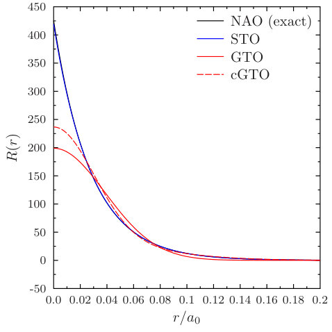 Figure 1
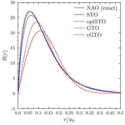 Figure 2
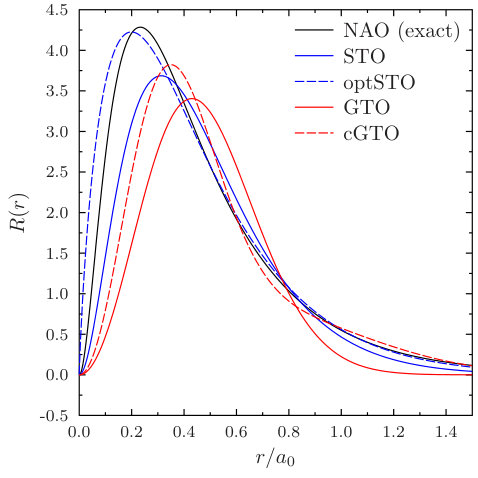 Figure 3
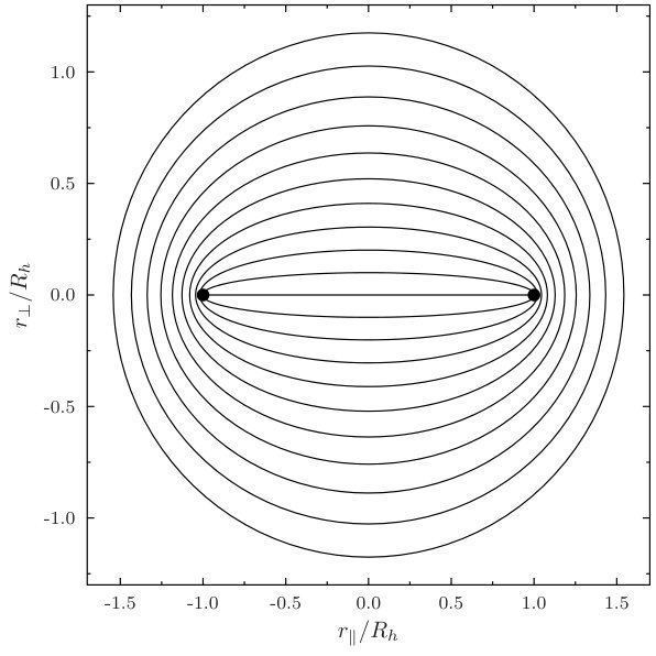 Figure 4
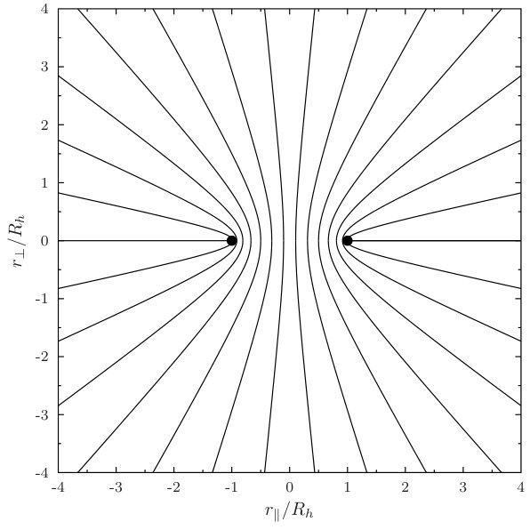 Figure 5
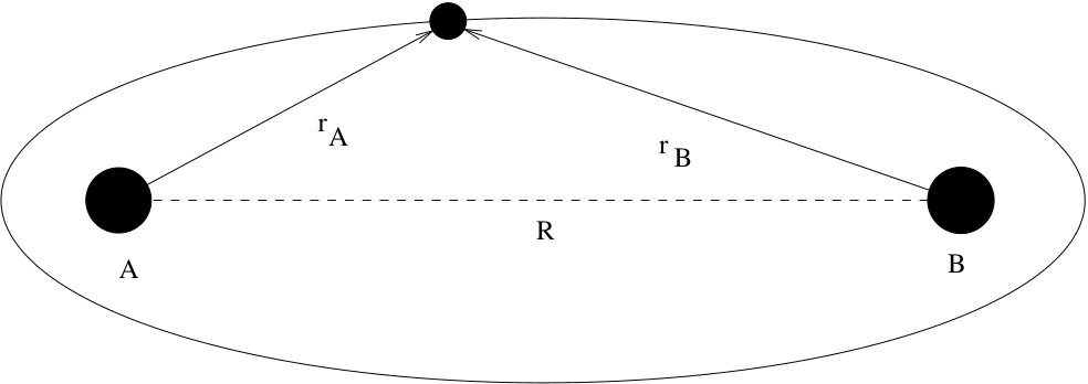 Figure 6
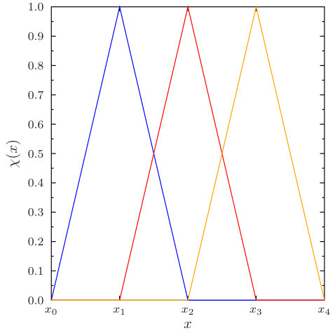 Figure 7
 Figure 8
Peer Reviews
No public reviews on file for this paper yet. If you reviewed it on a platform where reviews are public (OpenReview, ICLR, NeurIPS, ICML), you can paste yours below so the community can read it here.
Code & Models
Videos
No videos yet. Explain this paper in a talk, walkthrough, or lecture? Add one.
\RS@ifundefined
subsecref \newrefsubsecname = \RSsectxt
\RS@ifundefinedthmref \newrefthmname = theorem
\RS@ifundefinedlemref \newreflemname = lemma
\newrefsecname = section , names = sections , Name = Section , Names = Sections
\newrefsubsecname = section , names = sections
A review on non-relativistic, fully numerical electronic structure
calculations on atoms and diatomic molecules
Susi Lehtola
Abstract
The need for accurate calculations on atoms and diatomic molecules is motivated by the opportunities and challenges of such studies. The most commonly-used approach for all-electron electronic structure calculations in general – the linear combination of atomic orbitals (LCAO) method – is discussed in combination with Gaussian, Slater a.k.a.* *exponential, and numerical radial functions. Even though LCAO calculations have major benefits, their shortcomings motivate the need for fully numerical approaches based on, e.g. finite differences, finite elements, or the discrete variable representation, which are also briefly introduced.
Applications of fully numerical approaches for general molecules are briefly reviewed, and their challenges are discussed. It is pointed out that the high level of symmetry present in atoms and diatomic molecules can be exploited to fashion more efficient fully numerical approaches for these special cases, after which it is possible to routinely perform all-electron Hartree–Fock and density functional calculations directly at the basis set limit on such systems. Applications of fully numerical approaches to calculations on atoms as well as diatomic molecules are reviewed. Finally, a summary and outlook is given.
Department of Chemistry, University of Helsinki, P.O. Box 55 (A. I. Virtasen aukio 1), FI-00014 University of Helsinki, Finland
[TABLE]
1 Introduction
Thanks to decades of development in approximate density functionals and numerical algorithms, density functional theory1, 2 (DFT) is now one of the cornerstones of computational chemistry and solid state physics.3, 4, 5 Since atoms are the basic building block of molecules, a number of popular density functionals6, 7, 8, 9, 10 have been parametrized using ab initio data on noble gas atoms; these functionals have been used in turn as the starting point for the development of other functionals. A comparison of the results of density-functional calculations to accurate *ab initio *data on atoms has, however, recently sparked controversy on the accuracy of a number of recently published, commonly-used density functionals.11, 12, 13, 14, 15, 16, 17, 18, 19, 20, 21 This underlines that there is still room for improvement in DFT even for the relatively simple case of atomic studies.
The development and characterization of new density functionals requires the ability to perform accurate atomic calculations. Because atoms are the simplest chemical systems, atomic calculations may seem simple; however, they are in fact sometimes surprisingly challenging. For instance, a long-standing discrepancy between the theoretical and experimental electron affinity and ionization potential of gold has been resolved only very recently with high-level ab initio calculations.22 Atomic calculations can also be used to formulate efficient starting guesses for molecular electronic structure calculations via either the atomic density23, 24 or the atomic potential as discussed in ref. 25.
Diatomic molecules, in turn, again despite their apparent simplicity offer a profound richness of chemistry; ranging from the simple covalent bond in \ceH2 to the sextuple bonds in \ceCr2, \ceMo2, and \ceW2;26 and from the strong ionic bond in \ceNa+Cl- to the weak dispersion interactions in the noble gases such as \ceNe\bond…Ar. Even the deceivingly simple \ceBe2 molecule is a challenge to many theoretical methods, due to its richness of static and dynamic correlation effects.27 Counterintuitive non-nuclear electron density maxima can also be found in diatomic molecules, both in the homonuclear and heteronuclear case,28 again highlighting the surprising richness in the electronic structure of diatomic molecules. Going further down in the periodic table, diatomic molecules can be used to study relativistic effects to chemical bonding29, 30 as well as the accuracy of various relativistic approaches.31, 32, 33, 34, 35, 36, 37, 38, 39, 40, 41, 42, 43, 44, 45, 46, 47, 48, 49, 50, 51, 52 Although much of the present discussion applies straightforwardly to relativistic methodologies as well, they will not be discussed further in this manuscript. Instead, in the present work, I will review basic approaches for modeling the non-relativistic electronic structure of atoms and diatomic molecules to high accuracy *i.e. *close to the complete basis set (CBS) limit.
The organisation of the manuscript is the following. In 2, I will give an overview of commonly-used linear combination of atomic orbitals (LCAO) approaches. I will discuss both the advantages as well as the deficiencies of LCAO methods, the latter of which motivate the need for fully numerical alternatives, which are then summarized in 3. \SecrefApplications discusses applications of fully numerical approaches, starting out with a summary review on approaches for general molecules in 4.1, and continuing with a detailed review on the special approaches for atoms and diatomic molecules in LABEL:subsec:Atoms,_Diatomic-molecules, respectively. A summary and outlook is given in 5. Atomic units are used throughout the work.
2 LCAO approaches
In order to perform an electronic structure calculation, one must first specify the degrees of freedom that are allowed for the one-particle states a.k.a. orbitals of the many-electron wave function; that is, a basis set must be introduced. An overwhelming majority of the all-electron quantum chemical calculations that have been, and still are being reported in the literature employ basis sets constructed of atomic orbitals (AOs) through the LCAO approach.53, 54 As the name suggests, in LCAO the electronic single-particle states i.e. molecular orbitals of spin are expanded in terms of AO basis functions as
[TABLE]
where the index runs over all shells of all atoms in the system, denotes the distance , and is the center of the basis function that typically coincides with a nucleus. The matrix contains the molecular orbital coefficients, its rows and columns corresponding to the basis function and molecular orbital indices, respectively. The quantities , , and in (LABEL:LCAO) are the principal, azimuthal, and magnetic quantum numbers, respectively, of the AO basis functions
[TABLE]
where are radial functions, choices for which are discussed below in 2.2, and are spherical harmonics that are usually chosen in the real form.
The variational solution of the Hartree–Fock (HF) or Kohn–Sham2 equations within the LCAO basis set leads to the Roothaan–Hall or Pople–Nesbet equations55, 56, 57 for the molecular orbitals
[TABLE]
where is the (Kohn–Sham–)Fock matrix, is the overlap matrix, and is a diagonal matrix containing the orbital energies. Due to the interdependence of the Fock matrix and the molecular orbitals, (LABEL:Roothaan) has to be solved self-consistently, leading to the self-consistent field (SCF) approach. The iterative solution of (LABEL:Roothaan) starts from an initial guess for the orbitals, choices for which I have reviewed recently in ref. 25.
2.1 Benefits of LCAO approaches
LCAO calculations allow all electrons to be explicitly included in the calculation – even if it includes heavy atoms – without significant additional computational cost, as the necessary number of basis functions scales only in proportion to the number of electrons; the prefactor furthermore being very small. Moreover, since the AO basis functions tend to look a lot like real AOs, LCAO basis set truncation errors are often systematic, i.e. the error is similar at different geometries or spin states, for example. In such a case, even if the errors themselves are large, the relative error between different geometries or electronic states is usually orders of magnitude smaller, meaning that qualitatively correct estimates can typically be achieved with just a few basis functions per electron.
Due to the systematic truncation error, LCAO basis sets often allow good compromises between computational speed and accuracy, as basis sets of various sizes and accuracies are available. Single- basis sets may be used for preliminary studies where a qualitative level of accuracy suffices; for instance, for determining the occupation numbers in different orbital symmetry blocks, or the spin multiplicity of the ground state of a well-behaved molecule. Polarized double- or triple- basis sets are already useful for quantitative studies within DFT: thanks to the exponential basis set convergence of SCF approaches and to the fortunate cancellation of errors mentioned above, these basis sets often afford results that are sufficiently close to the CBS limit. Quadruple- and higher basis sets are typically employed for benchmark DFT calculations, for the calculation of molecular properties that are more challenging to describe than the relative energy, as well as for post-HF calculations which require large basis sets to reproduce reliable results.
Again allowed by the small number of basis functions, post-HF methods such as Møller–Plesset perturbation theory58, configuration interaction (CI) theory and coupled-cluster (CC) theory59 can often be applied in the full space of molecular orbitals in LCAO calculations. Because of this, the use of post-HF methods becomes unambiguous, allowing the definition of trustworthy model chemistries60 and enabling their routine applications to systems of chemical interest.
Finally, once again facilitated by the small number of basis functions, several numerically robust methods are tractable for the solution of the SCF equations of (LABEL:Roothaan) within LCAO approaches. As the direct iterative solution of (LABEL:Roothaan) typically leads to oscillatory divergence, the solution of the SCF problem is traditionally stabilized with techniques such as damping,61 level shifts,62, 63, 64 or Fock matrix extrapolation65, 66 in the initial iterations. Once the procedure starts to approach convergence, the solution can be accelerated with e.g. the direct inversion in the iterative subspace (DIIS) method,67, 68 or approached with true69, 70, 71, 72, 73, 74, 75, 76, 77, 78 or approximate79, 80, 81, 82 second-order orbital rotation techniques that converge even in cases where DIIS methods oscillate between solutions. For more information on recently suggested Fock matrix extrapolation techniques, I refer to refs. 83, 84, 85 and references therein.
2.2 Variants of LCAO
Three types of LCAO basis sets are commonly used. First, consider the Slater-type orbitals86, 87, 88 (STOs), which are also commonly known as exponential type orbitals (ETOs)
[TABLE]
STOs were especially popular in the early days of quantum chemistry, since they represent analytical solutions to the hydrogenic Schrödinger equation. The STO atomic wave functions tabulated by Clementi and Roetti89 should especially be mentioned here due to their wealth of applications. For instance, their wave functions are still sometimes used for non-self-consistent benchmarks of density functionals.90, 91, 9
STOs have the correct asymptotic form both at the nucleus – the Kato cusp condition92 can be satistied – as well as far away, where the orbitals should exhibit exponential decay.93, 94, 95 However, STOs are tricky for integral evaluation in molecular calculations, typically forcing one to resort to numerical quadrature.96, 97, 98, 99 Note that even though STO basis sets with non-integer values100, 101, 102, 103 have been shown to yield significantly more accurate absolute energies than analogous basis sets that employ integer values for ,104, 105, 106, 107, 108, 109 they have not become widely used. Closely related to STOs, Coulomb Sturmians110, 111 have recently gained renewed attention but have not yet become mainstream, see e.g. refs. 112 and 113 and references therein.
Second, Gaussian-type orbitals (GTOs)
[TABLE]
enjoy overwhelming popularity thanks to the Gaussian product theorem114 that facilitates the computation of matrix elements, which is especially beneficial for the two-electron integrals,115, 116, 117 the calculation of which is typically the rate determining step in SCF calculations. The importance of efficient, analytical evaluation of molecular integrals can hardly be overstated. Efficient integral evaluation makes calculations affordable: it has long been possible to use large atomic basis sets and/or study large systems with Gaussian basis sets. Analytical integral evaluation guarantees accuracy: it is straightforward to calculate e.g. geometric derivatives and reliably estimate force constants and vibrational frequencies, because the matrix elements are numerically stable.
Another reason for the popularity of GTOs was the recognition early on that STOs can in principle be expanded exactly in GTOs;118 thus, for instance, the hydrogenic atom can be solved with GTO expansions with controllable accuracy, highlighting the flexibility of Gaussian basis sets.119 Indeed, most commonly-used quantum chemistry programs, such as refs. 120, 121, 122, 123, 124, 125, 126, 127, 128, 129, 130 to name a few, employ Gaussian basis sets such as the Pople 6-31G131, 132, 133, 134, 135, 136, 137, 138, 139, 140 and 6-311G series,141, 142 the Karlsruhe def143, 144 and def2 series,145, 146 the correlation consistent cc-pVXZ series by Dunning, Peterson, and coworkers,147, 148, 149, 150, 151, 152, 153, 154, 155, 156, 157, 158 the polarization consistent pc- and pcseg- series by Jensen,159, 160, 161, 162, 163, 164, 165, 166 the ZaPa sets by Petersson and coworkers,167, 168 as well as the atomic natural orbital (ANO) basis sets by Almlöf, Roos, and coworkers;169, 170, 171, 172, 173, 174, 175, 176, 177, 178, 179, 180 see e.g. refs. 181, 182, 183 for reviews on Gaussian basis sets.
Third, numerical atomic orbitals (NAOs)
[TABLE]
are the most recent addition to the field.184, 185, 186, 187 Unlike GTOs and STOs, NAOs have no analytical form; instead, NAOs are typically pretabulated on a radial grid. (Note that adaptive approaches employing flexible NAOs have also been suggested but have not become commonly used;188, 189, 190, 191, 192 the atomic radial grid approach should also be mentioned in this context.193, 194)
The NAO form is by definition superior to GTOs or STOs: a suitably parametrized NAO basis set is able to represent GTOs and STOs exactly, while the opposite does not hold. Thanks to this great flexibility, unlike GTOs or STOs, a minimal NAO basis set can be an exact solution to the noninteracting atom at the SCF level of theory: a single NAO can simultaneously satisfy both the Kato cusp condition at the nucleus and have the correct exponential asymptotic behavior.
In further contrast to primitive i.e. uncontracted STO and GTO basis sets, single-center NAOs can be defined at no additional cost to be orthonormal, which leads to better conditioned equations even for the molecular case. These features make NAOs the most accurate LCAO basis set, as has been recently demonstrated in multiple studies both at the SCF and post-HF levels of theory.195, 196, 197, 198 Alike STOs, NAOs require quadrature for molecular integral evaluation, but this does not appear to be a problem on present-day computers.199, 195 NAOs are typically constructed from SCF calculations on atoms, which will be reviewed in the next section.
2.3 Case study: Kr atom; contracted basis sets
A comparison of the three types of basis functions for an exchange-only local density calculation on the krypton atom is shown in 1 for the atomic , , and orbitals. Here, the NAOs are chosen as the exact , , and orbitals, whereas the STO and GTO functions have been optimized for best overlap with the exact orbital.
The STO form clearly allows an accurate expansion of the orbital. The , however, is a special case, as it experiences the least screening by the other electrons. These screening effects deform the orbital from the hydrogenic STO form, and become more visible for the and orbitals: for , the STO orbital is already quite dissimilar from the exact one. But, as was discussed above in 2.2, relaxing the restrictions in the STO form from and for the and orbitals, respectively, to also allow fractional leads to significant improvements in the accuracy of the STO orbitals, as can be seen in 1.
There are large differences between the GTO and the exact orbitals, which are especially clear for the orbital which should have a cusp at the origin. However, the accuracy of the GTO basis set can be radically improved by adding more functions. \Figrefbasis-comparison also shows results for contracted GTO (cGTO) basis functions, which have been formed from two GTO primitive functions by optimizing the primitives and their expansion coefficients for the best overlap with the exact orbital. The cGTO basis set can be made more and more accurate by adding more and more primitives to the expansion.
However, it is worth pointing out here that in a sense, cGTOs are also a form of a NAO basis. Employing general contractions,200 the single-center basis functions can be chosen to be strictly orthonormal, and non-interacting atoms can be solved to high accuracy in a minimal basis set that is assembled from a large number of primitive Gaussians. Alike NAOs, efficient integral evaluation in generally contracted GTO (gcGTO) basis sets is significantly more complicated than in primitive or segmented Gaussian basis sets, since a primitive integral can contribute to several contracted integrals.
gcGTO basis sets are typically formed from ANOs, and they are well-known to yield faster convergence to the basis set limit with respect to the number of basis functions than uncontracted basis sets or basis sets employing segmented contractions.169, 170, 171, 201, 172, 173, 202, 174, 175, 176, 177, 178, 179, 180, 203 Even though gcGTOs are similar to NAOs, the number of degrees of freedom in any Gaussian basis set expansion is much smaller than what is possible with a true NAO basis set: large Gaussian basis sets for heavy atoms typically contain up to 30 or 40 primitives per angular momentum shell, whereas NAOs are often tabulated with hundreds to thousands of radial points. As NAOs allow for a more accurate description of atomic orbitals than Gaussian expansions do, while ANOs yield faster convergence in post-HF calculations than basis sets constructed from HF orbitals do, it is clear that it should be possible to form extremely efficient numerical ANO (NANO) basis sets for post-HF studies. The generation of NANO basis sets could follow pre-established procedures to generate ANOs from Gaussian expansions; suitable fully numerical implementations of the multiconfigurational approaches that are typically used to construct ANOs have been described in the literature, as is discussed below in 4.2.
2.4 Deficiencies of LCAO approaches
In the case of atomic calculations, it is relatively straightforward to obtain near-CBS limit energies even with LCAO basis sets: since only a single expansion center is involved, the basis set is relatively well-conditioned even if large basis set expansions are used. However, the basis set requirements depend not only on the level of theory and property; they may also depend on the studied state.
For some properties, it is possible to explicitly identify the regions of the basis set that require extra focus: for instance, the Fermi contact term for a nucleus A is proportional to , where is the distance from nucleus, so an accurate reproduction of the electronic structure at the nucleus is necessary. Because only orbitals are non-zero at the nucleus, the accuracy of the description of the contact term is mostly dependent on the tight functions.
Other examples include the polarization induced by weak electric and/or magnetic field perturbations, for which analytic expressions can be derived for the change in the atomic orbitals. Equipped with this knowledge, one can parametrize perturbation-including basis sets both in the case of STOs204, 205, 206 and GTOs207, 208, 209, 210, 211, 212, 213, 214, 215, 216, 217, 205, 218, 219, 220, 221 which achieve faster convergence to the basis set limit than the non-perturbation-including basis sets. Similarly, knowledge on the asymptotic long-range behavior of the wave function94, 95 can be used to construct GTO basis sets with improved asymptotic behavior.222
Completeness-optimization223, 224 is a general approach that may be used to parametrize basis sets that yield near-CBS values for the energy and/or whatever molecular properties. The approach does not make any assumptions on the level of theory or specific properties that are calculated; instead, the only assumption is that the property can be converged with a sufficiently large basis set. The approach relies on an iterative approach where new basis functions are added one by one, until the property has converged. Completeness-optimization has been demonstrated so far for electric and magnetic properties,223, 225, 226, 227, 228, 229, 230, 231, 232, 233, 234, 235, 224 electron momentum densities,236, 237 as well as NAO simulations of nanoplasmonics.238
However, getting to the CBS limit can still be painstaking, as several sets of tight and/or diffuse functions may be necessary to achieve converged results.239, 150, 240, 241, 242 For instance, Gaussian primitives with exponents as small as have been found necessary to make \ceF- properly bound at the DFT level.243 Basis sets with a fixed analytic form also pose intrinsic limits to their accuracy because of their incorrect asymptotic behavior. This has been shown in the case of Gaussian basis sets e.g. for the moments of the electron momentum density,244, 236, 237 the electron density,245, 246, 247, 248 as well as nuclear magnetic properties.249 Reaching the CBS limit for such properties may be untractable unless more flexible basis sets are employed.
Molecular calculations are even more difficult than atomic ones. Although it is straightforward to establish a hierarchy between NAO, STO, and GTO basis sets in the case of atoms and optimize basis sets for them, atomic symmetries are broken by the molecular environment, requiring the addition of polarization functions into the atomic basis set. It is generally acknowledged that the optimal form of polarization functions is not known, and that the ranking of GTOs *vs *STOs *vs *NAOs is not clear in the case of polarization functions. Indeed, GTO and STO polarization functions are commonly employed in NAO calculations.250, 195
Another complication is that the set of AO basis functions placed on the various nuclei may develop linear dependencies. Linear dependencies are especially problematic for diffuse basis functions, whereas tight functions are less problematic since they are highly localized. Thus, it is especially difficult to accurately reproduce molecular properties that are sensitive to the diffuse part of the wave function with LCAO approaches; further complications may also be caused by the limitations in the form of the AO basis functions discussed above.245, 244, 246, 247, 248, 236, 237, 249
Any linear dependencies that exist in the basis set are typically removed via the canonical orthonormalization procedure251 in order to make the basis unambiguous. In such a case, a calculation with a smaller basis set can reproduce the same or a lower energy than the one predicted by the calculation with the linearly dependent basis.
There are workarounds to this problem for some cases. Instead of using a large basis set on each of the nuclei, one can employ bond functions: use a smaller basis on the nuclei while placing new basis functions in the middle of chemical bonds; such a procedure can yield faster convergence to the basis set limit.252 Moreover, one can replace diffuse functions placed on every atom with ones placed only on the molecular center of symmetry. However, in either case, the optimal division and placement of functions to recover the wanted property yet keep linear dependencies at bay may be highly nontrivial for a general system, and is clearly dependent on the molecular geometry.
A general approach for avoiding the problems with linear dependencies that arise from diffuse functions in a molecular setting has, however, been suggested. In this approach, diffuse functions are modeled by a large number of non-diffuse functions placed all around the system.253, 254 The use of such lattices of Gaussian functions is an old idea, originally proposed as the “Gaussian cell model” by Murrell and coworkers.255 The Gaussian cell model was later revisited by Wilson and coworkers, who showed that much better results can be obtained by supplementing the lattice basis set with AO functions on the nuclei.256, 257, 258 The authors of refs. 253 and 254 appear to have been unaware of the work by Murrell, Wilson, and coworkers. Nonetheless, the Gaussian cell model is but an imitation of proper real-space methods: the use of a grid of spherically symmetric Gaussians clearly cannot yield the same amount of accuracy or convenience as a true real-space approach that employs a set of systematically convergent basis functions with finite support. In one dimension, however, arrays of Gaussian functions called gausslets have been recently shown to yield useful completeness properties.259 But, it is not yet clear how well the gausslet approach can be generalized to atoms heavier than hydrogen, or to general three-dimensional molecular structures.
The accurate calculation of *e.g. *potential energy surfaces is also complicated in the LCAO approach due to the so-called basis set superposition error (BSSE). can be underestimated with respect to and , because the locality of the electrons onto the basis functions belonging to the fragments is not enforced. Although BSSE can be approximately removed with the Jansen–Ros–Boys–Bernardi counterpoise correction260, 261 or developments thereof,262, 263, 264, 265, 266, 267 and although BSSE becomes smaller when going to larger atomic basis sets, it is not always clear how accurate the obtained interaction energies are. The geometry-dependence of the molecular basis set also complicates the calculation of molecular geometries and vibrational frequencies, as Pulay terms268 appear.
Finally, it is difficult to improve the description of the wave function in an isolated region of space in the LCAO approach. The addition of a new function to describe *e.g. *the wave function close to the nucleus requires changing the solution globally to maintain orbital orthonormality, because the basis functions are non-orthogonal and have global support. Could these problems be circumvented somehow?
3 Real-space methods
An alternative to the use of LCAO basis sets is to switch to real-space methods, where the basis functions no longer have a form motivated purely by chemistry. Instead of expanding the orbitals in terms of AOs as in (LABEL:LCAO), the expansion is generalized to
[TABLE]
where the real-space basis set can be chosen based on convenience for the problem at hand. For illustration, a simple option is to form the three-dimensional basis set as a tensor product of one-dimensional basis functions as
[TABLE]
where the can in turn be chosen as *e.g. *the hat functions shown in 2. In many dimensions, also other kinds of choices for the three-dimensional basis functions can be made instead of the rectangular elements of (LABEL:tensorbasis): for instance, triangles in two dimensions, or tetrahedra, hexahedra, or prisms in three dimensions; more information on these can be found in any standard finite element textbook such as ref. 269.
The present work focuses on fully numerical calculations on atoms and diatomic molecules. As will be reviewed below in 4, a one-dimensional treatment is sufficient for atoms, whereas diatomic molecules require a two-dimensional solution. Almost all the diatomic approaches reviewed below use a rectangular basis similar to (LABEL:tensorbasis):
[TABLE]
where and are prolate spheroidal coordinates introduced below in 4.3. The only exception is the program by Heinemann, Fricke and Kolb which employs triangular elements as discussed in ref. 270; the present discussion can thus be restricted to the case of (LABEL:tensorbasis) or (LABEL:2Dbasis). Now, as the basis factorizes in the coordinates, it is sufficient to restrict the discussion to one dimension, as the generalization to many dimensions is obvious.
Four kinds of numerical approaches are commonly used for the one-dimensional basis functions : finite differences, finite elements, basis splines, and the discrete variable representation. The common feature in all the approaches is that a function is represented in terms of the basis functions as
[TABLE]
As will be seen below, the first three methods rely on a local piecewise polynomial representation for , whereas the last one can also be formulated in terms of non-polynomial basis functions . All approaches should yield the same value at the CBS limit – this is what makes fully numerical approaches enticing in the first place.
However, as will be discussed below, the speed of convergence to the CBS limit depends heavily on the order of the used numerical approximation, with higher-order methods affording faster convergence in the number of basis functions than lower-order methods. This means that comparing the accuracy of the various approaches is not trivial, as even the same approach can manifest different convergence properties when implemented at different orders.
Furthermore, the speed of convergence also depends in each case on the system, the studied property, and the level of theory used in the calculation: HF and DFT afford exponential converge in the basis set, whereas post-HF methods only exhibit polynomial convergence if the orbital space is not fixed. For this reason, for numerical results I refer the reader to the individual references listed in 4.
3.1 Finite differences
The finite difference method is arguably the oldest and the best-known method for numerically solving differential equations. The method is based on a Taylor expansion of as
[TABLE]
where it is assumed that is tabulated on a grid as , where is the grid spacing; that is, . From the Taylor expansion, (LABEL:taylor), one can obtain approximations for the derivatives of , for instance, using central differences as
[TABLE]
these are known as the two-point and three-point stencils, respectively. The procedure can also be done at higher orders, leading to *e.g. *the four- and five-point rules
[TABLE]
which carry a smaller error, as evidenced by the smaller remainder term. Finite difference formulas can be easily generated to arbitrary order by recursion, even on nonuniform grids.271
An important feature of the finite difference method is that relaxation approaches can be formulated for Schrödinger-type equations. For instance, applying (LABEL:df-twop) onto
[TABLE]
one obtains
[TABLE]
which can be rearranged into the relaxation equation
[TABLE]
that can be solved by iteration. Furthermore, the iteration can be made faster by the use of the successive overrelaxation method
[TABLE]
where corresponds to relaxation and to overrelaxation.
Although the relaxation approach is straightforward and readily applicable to high-performance computing, the drawback is that a good initial guess is necessary for the solution as well as the eigenvalue . Another drawback is that, as can be seen from (LABEL:fi-relax), information is passed only locally, and so the relaxation becomes extremely slow in fine meshes; this can be, however, circumvented with multigrid approaches272 that pass information simultaneously at multiple length scales, thus avoiding the slowdown.
It is also possible to avoid using relaxation approaches altogether: finite difference calculations can be written as matrix eigenvalue problems, e.g. (LABEL:fd-schr-threep) can be rewritten as
[TABLE]
and the finite-difference Hamiltonian is given by the banded-diagonal matrix
[TABLE]
where and are vectors of the values of the wave function and the potential, respectively; however, this is rarely done in practice, as the basis spline and finite element methods described below naturally lead to matrix equations.
Having obtained approximate derivatives of the function in the vicinity of the current point using *e.g. *(LABEL:df-twop,_d2f-threep) or (LABEL:df-fourp,_d2f-fivep), (LABEL:taylor) expands the description of the function beyond the known values to how the function behaves in-between the grid points. From the form of (LABEL:taylor), it is clear that the finite difference method in fact corresponds to a local, piecewise polynomial basis for . However, the Taylor rule of (LABEL:taylor) implies that a different polynomial is used for every grid point , which leads to a discontinuous representation for . This is the puzzle of the finite difference method: it is not obvious how the approximated function behaves in-between grid points.
Applications to quantum mechanics require matrix elements that involve spatial integrals; thus, a quadrature rule is necessary, but due to the aforementioned ambiguity, it is not possible to derive one from the finite difference formulation. Instead, the typical solution is to just use quadrature formulas such as Newton–Cotes, which can be derived from Lagrange interpolating polynomials, yielding e.g. the two-point trapezoid rule, the three-point Simpson’s rule, and the five-point Boole’s rule. Although these quadrature formulas imply using the same fitting polynomial for all points in the fitting integral – contrasted to using different polynomials at every point to get the derivatives according to \eqrangerefdf-twopd2f-fivep – there is a solid mathematical argument for using such a hybrid scheme:* *the error bounds. For instance, the trapezoid and Simpson’s rules have errors of and , respectively, which can be contrasted with the and errors for the derivatives in (LABEL:df-twop,_d2f-threep) or (LABEL:df-fourp,_d2f-fivep), respectively. Because of this, the mismatch between the rules for derivation and integration is not a problem in practice: numerical integration is more accurate than numerical differentiation, and an arbitrary level of accuracy is anyhow achievable by using a finer grid .
Still, getting to the CBS limit is complicated by the lack of variationality in finite difference calculations:273 when the variational principle does not hold, calculations with a smaller can yield an increased energy, even though a better basis set is used. This error is caused by the underestimation of the kinetic energy by the finite difference representation of the Laplace operator.274, 275
But, finite difference electronic structure calculations often have also another, even larger source of non-variationality than the kinetic energy approximation: aliasing error in the Coulomb and exchange potentials. This error arises whenever the electron density is expressed in the same grid as the molecular orbitals
[TABLE]
because an order- polynomial wave function yields a density that has an order- polynomial expansion, which ends up being truncated. The aliasing error is analogous to the error of resolution-of-the-identity approaches of LCAO methods:276, 277, 278, 279, 280 it makes the classical Coulomb interaction between the electrons less repulsive, and the exchange interaction less attractive. The latter error yields a slight increase of the energy, but the former error makes the energy too negative, resulting in energies that are underestimated i.e. anti-variational until the grid is made fine enough.
One more limitation in the finite difference method is that if an equispaced grid is used, higher-order rules which are based on high-order polynomials become unstable due to Runge’s phenomenon.281 For this reason, for instance the x2dhf program282, 283, 284 discussed below in 4.3 employs eight-order *i.e. *9-point central difference expressions for computing second derivatives with error, and a 7-point rule for quadrature with error.283
3.2 Explicit basis set methods
Instead of invoking a local piecewise polynomial basis only implicitly like in the finite difference method, the finite element method (FEM) explicitly uses a piecewise polynomial basis set to represent the function like in interpolation theory. Because of this, it can be remarked that finite differences approximate the Schrödinger equation, while finite elements – as well as basis splines and the discrete variable representation – approximate its solution. The nice thing about these three approaches is that the basis is fully defined: evaluating the function or its derivatives at an arbitrary point is completely unambiguous, meaning e.g. that adaptive quadrature rules, or rules relying on points other than the discretization nodes can be easily employed. Moreover, because an unambiguous basis set has now been defined, instead of relying on an (over)relaxation approach as in the finite difference method, one may use the same variational techniques as in LCAO approaches to solve for the wave functions, e.g. the Roothaan–Hall equation of (LABEL:Roothaan).
In the finite element method, the domain for is divided into into line segments called elements , and a separate, local polynomial basis is defined within each element. The basis functions within an element, commonly known also as shape functions, are determined by choosing points called nodes within the element, .
In the most commonly used finite element variant, one demands that the value of at each node is given by a specific basis function
[TABLE]
Employing a polynomial expansion for , one sees that the shape functions for nodes are order polynomials. Especially, the condition in (LABEL:fem) is fulfilled by Lagrange interpolating polynomials (LIPs)
[TABLE]
which are well-known to yield the error estimate
[TABLE]
Nodes are typically placed also at the element boundaries. Because the node at the element boundary is shared by the rightmost function in the element on the left, and the leftmost function in the element on the right, these two basis functions have to be identified with each other, guaranteeing continuity of across the element boundary. For instance, the hat functions in 2 correspond to two-node elements, where both nodes are on element boundaries.
Because all shape functions are fully localized within a single element, it is very easy to take advantage of this locality in computer implementations. Moreover, the correspondence of functions belonging to nodes at element boundaries can be easily handled in computer implementations by index manipulations, i.e. overlaying.
In this formulation, because all basis functions are smooth, will also be smooth within each element, and the function is guaranteed to be continuous over element boundaries. However, while all derivatives are guaranteed to be continuous within an element, discontinuities in the first derivative may be seen at the element boundaries.
Although the continuity of the derivative(s) can be strictly enforced by straightforward extension of the approach in (LABEL:fem), in which the description of the values of and at the nodes are each identified to arise from a single shape function, this does not appear to be necessary in typical applications to quantum mechanics. The reason for this is the variational principle: discontinuities in the derivative imply a higher kinetic energy. The derivatives of the Lagrange interpolating polynomials, (LABEL:LIP), do not vanish at the nodes, and this flexibility gives the variational principle room to try to match the derivatives across element boundaries.
Although the Runge phenomenon281 is also a problem for the finite element method with uniformly spaced nodes within the element, the method can be made numerically stable to high orders if one employs non-uniformly spaced nodes; suitable choices include Gauss–Lobatto nodes, or Chebyshev nodes as in the spectral element method.285 The benefit of high-order elements is apparent in 25: the errors become small rapidly in increasing element order.286 If in addition to defining the shape functions, the same rule is also used for quadrature, one obtains a discrete variable representation (DVR) which will be discussed in more detail below.
In addition to varying the location of the nodes within each element to make high-order rules numerically stable, it is possible to use elements of different sizes and orders within a single calculation, granting optimal convergence to the basis set limit with the least possible number of basis functions; this is the origin for the popularity of FEM across disciplines. For more discussion on the finite element method, including other kinds of shape functions than Lagrange interpolating polynomials, I refer to my recent discussion in ref. 286.
Like the finite element method, basis splines (B-splines) are piecewise polynomials, with an order spline corresponding to a polynomial function of order . B-splines were originally developed by Schoenberg,287 and were introduced in the context of atomic calculations by Gilbert and Bentoncini,288, 289, 290, 291 based on earlier work on their application to single-particle problems by Shore.292, 293, 294, 295, 296 B-splines are defined by knots , which need not be uniformly spaced, with the Cox–de Boor recursion
[TABLE]
thus, are piecewise constants, are hat functions (2), and so on. On each interval , only B-splines are non-zero. This means that computational implementations of B-splines and finite elements share similar aspects: matrix elements are computed in batches on the individual knot intervals; only the indexing of the basis functions is different. B-splines and their applications to atomic and molecular physics have been reviewed by Bachau in ref. 297, to which I refer for further details.
The DVR,298, 299, 300, 301, 302, 303, 304 in turn, is conventionally based on orthogonal polynomial bases and their corresponding quadrature rules,300, 301 underlining a strong connection to the finite element and B-spline approaches. Generalizations of DVR to non-polynomial bases have been suggested by Szalay305, 306, 307, 308 and Littlejohn, Cargo and coworkers309, 310, 311, 312, 313, 314. The DVR community discerns between a variational basis representation (VBR), in which all operator matrix elements i.e. integrals are computed exactly i.e. analytically, a finite basis representation (FBR), in which a quadrature rule is employed to approximate the integrals like in FEM, and the DVR itself in which a unitary transformation of the FBR basis set, which is often delocalized, is used to obtain an effectively localized basis which affords a diagonal approximation for matrix elements as
[TABLE]
this is the famous “discrete property” of DVR. Although the DVR approach offers few benefits for one-dimensional problems over the full, variational treatment, since cost of the additional transformation has similar scaling to the savings, the approach becomes extremely powerful in many dimensions due to the diagonality of potential operators, (LABEL:O-diag).
The DVR is commonly used on top of a finite element treatment, yielding the FEM-DVR method, as discussed e.g. by Rescigno and McCurdy.315 Indeed, the DVR approaches discussed in the rest of the manuscript all employ Lobatto elements, which use a basis of Lagrange interpolating polynomials defined by a set of Gauss–Lobatto quadrature nodes, as was discussed above in relation to FEM. It is easy to see that if the same Gauss–Lobatto quadrature rule is used both to define the finite element basis and for evaluating matrix elements, then the property of the interpolating polynomials, (LABEL:fem), directly leads to the diagonal approximation of matrix elements, (LABEL:O-diag).
However, this is an approximation: reliable computation of the matrix elements in 28 may require using more than quadrature points, which in turn may introduce off-diagonal elements in the matrix representation of . Because of this quadrature error, which is analogous to the aliasing error discussed above in the case of finite-difference calculations, DVR calculations can be non-variational; however, the error can be made smaller and smaller by going to a larger DVR basis sets.
4 Applications
4.1 Overview on general approaches for arbitrary molecules
With the ability to use varying levels of accuracy for different parts of the system in the real-space basis set, even challenging parts of the wave function, such as at the nucleus or far away from it, can be straightforwardly converged to arbitrary accuracy. Real-space methods thereby grant straightforward access even to properties that are difficult to calculate accurately with *e.g. *Gaussian basis sets, such as nuclear magnetic properties, the electron density close to, or at the nucleus, as well as the electron momentum density. A further benefit of real-space methods is that the locality of the real-space basis set allows for easy and efficient use of the algorithms even on massively parallel architectures, whereas LCAO calculations are not as nearly straightforward to parallellize to thousands of processes.
Achieving the CBS limit is simple in real-space methods. Due to the local support of the basis functions, the basis set never develops linear dependencies, so the CBS limit can be achieved simply by increasing the accuracy of the real-space basis set until the result does not change anymore. The drawback to the arbitrary accuracy is that the number of basis functions necessary for achieving even a qualitative level of accuracy in real-space approaches is significantly larger than in the LCAO approach; the crossover typically happens only at high precision.
The number of basis functions in real-space methods is especially large in all-electron calculations, as disparate length scales are introduced by the core orbitals. The description of the tightly bound core orbitals necessitates an extremely robust basis near the nuclei, whereas a much coarser basis is sufficient for the valence electrons. One option to circumvent this problem is to forgo all-electron calculations and to approximate the core electrons with pseudopotentials316, 317, 318, 319, 320, 321, 322 or projector-augmented waves323 (PAWs), making the problem accessible to a number of fully numerical approaches; see e.g. refs. 324, 273, 325, 326, 327 for references. However, as the present review focuses on all-electron calculations, the use of projector-augmented waves and pseudopotentials will not be considered in the rest of the manuscript.
In order to make all-electron a.k.a. full-potential calculations feasible, a suitable representation has to be picked for the description of the core electrons. As was stated above, LCAO calculations have problems especially with diffuse parts of the wave function, wheras core orbitals don’t pose significant complications. Vice versa, real-space methods tend to struggle with core orbitals, but are well-adapted to the description of diffuse character. This has lead to approaches that hybridize aspects of LCAO and real-space calculations.193, 328, 329, 330, 331, 191, 332, 333, 334, 335, 336, 337, 338, 339, 340 By representing the core electrons using an atom-centric radial description, a significantly smaller real-space basis set may suffice, making the approaches scalable to large systems while still maintaining a very high level of accuracy. In a somewhat similar spirit, the multi-domain finite element muffin-tin and full-potential linearized augmented plane-wave + local-orbital approaches have also been recently shown to afford high-accuracy all-electron calculations for molecules.341, 342
However, several methods that are able to solve the all-electron problem without using an LCAO component exist as well. First, the FEM allows for calculations at arbitrary precision even at complicated molecular geometries by employing spatially non-uniform basis functions. A number of FEM implementations for all-electron HF or DFT calculations on molecules or solids with arbitrary geometries have been reported in the literature.343, 344, 345, 346, 347, 348, 349, 350, 351, 352, 353, 354, 355, 356, 357, 358, 359, 360, 361 Another solution is to use grids with hierarchical precision362, 363 or adaptive multiresolution multiwavelet approaches324, 364, 365, 366, 367, 368, 249, 198 that are under active development and which have recently achieved microhartree-accuracy in molecular calculations, even at the post-HF level of theory.369, 370, 371, 372 Regularization of the nuclear cusp373, 374, 375 and approaches employing adaptive coordinate systems376 also have been suggested.
The considerably larger number of basis functions in real-space approaches compared to LCAO calculations means not only that more computational resources – especially memory and disk space – are needed, but also that alternative approaches for e.g. the solution of the SCF equations have to be used. For instance, employing 100 degrees of freedom such as grid points per Cartesian axis yields basis functions in total. The corresponding Fock matrix would formally have a dimension , requiring a whopping 8 terabytes of memory (assuming double precision), and making its exact diagonalization untractable. Naturally, these challenges become even worse for molecules for which orders of magnitude more points are necessary.
Furthermore, the calculation of properties may be complicated in real-space methods. If the numerical basis set is independent of geometry, there is no basis set superposition error as in LCAO calculations. Instead, one has to deal with the infamous “egg-box effect”,377 which is caused by the use of a finite spatial discretization that breaks the translational and rotational symmetries of the system. Then, the numerical accuracy depends on the relative position of the nuclei to the discretization, which can manifest as *e.g. *spurious forces.377 The egg-box effect can be made small by going to larger and larger basis sets; other alternatives have been discussed in ref. 378, but the best approach may depend on the form of the numerical basis set.
Typical real-space approaches employ local basis functions such as the ones in 2, making most matrices extremely sparse. Large-scale computational implementations are possible only via the exploitation of this sparsity. For instance, the Coulomb interaction as well as local and “semilocal” density functionals require only local information, namely, the Coulomb potential at every grid point, as well as the exchange-correlation potential that is built from the density (and possibly its gradient) at every grid point. In contrast, the exact Hartree–Fock exchange interaction is non-local; however, it can be truncated to finite range in large systems, especially if exact exchange is only included within a short range, as in the popular Heyd–Scuseria–Ernzerhof functional.379, 380 Alternatively, the evaluation of exact exchange can be sped up with projection operators;381, 382 or the Krieger–Li–Iafrate (KLI) approximation383, 384 can be used to build a fully local exchange potential, also allowing exact-exchange calculations on large systems.385, 386, 387, 388 Further necessary steps in the implementation of large-scale real-space approaches involve replacing the full matrix diagonalization in the conventional Roothaan orbital update of (LABEL:Roothaan) with an iterative approach such as the Davidson method389 that is used to solve only for the new occupied subspace, or avoiding diagonalization altogether by using e.g. Green’s function methods to solve for the new occupied orbitals, as in the Helmholtz kernel method.390, 391, 392, 335
So far, the discussion has been completely general. Next, I shall discuss calculations on atoms and diatomic molecules. Although it is possible to obtain accurate results for atoms or diatomic molecules by employing general three-dimensional real-space approaches as the ones discussed above – see e.g. refs. 393 and 394 for tetrahedral-element calculations on \ceH2+, and \ceH- and \ceHe, respectively – they carry a higher computational cost. A specialized implementation is able to treat some dimensions analytically or semianalytically, whereas these dimensions need to be fully described in the general three-dimensional programs, necessitating orders of magnitude more degrees of freedom to achieve the same level of accuracy as is possible in the specialized algorithms.
For instance, while a grid can be assumed to yield a decent HF or KS energy for any atom, an atomic solver will likely give a much better energy with just basis functions, as the angular expansion for to electrons requires but 16 spherical harmonics, while 60 radial functions afford sub-microhartree accuracy even for xenon.286 Furthermore, the smaller basis set afforded by the use of the symmetry inherent in the problem allows (di)atomic calculations to use a diversity of powerful approaches – such as the use of (LABEL:Roothaan) with full diagonalization for the orbital update – which are not tractable in the general three-dimensional approach.286, 395
4.2 Atoms
At the non-relativistic level of theory, the electronic Hamiltonian for an atom with nuclear charge
[TABLE]
commutes with the total angular momentum operator , its component , as well as the total spin operator . As a result, electronic states are identified with the term symbol , where the total electronic angular momentum is one of . In cases where the term symbol is not , the wave function is in principle strongly correlated due to the degeneracy of partially filled shells. Unlike the molecular case, in which the treatment of strong correlation effects is still under active research, for atoms strong correlation effects are much more docile due to the limited number of accessible orbitals. For example, in the ground state configuration of boron the shell only has a single electron, which should be distributed equally between the , and orbitals, yielding a multiconfigurational (MC) wave function. A good symmetry-compatible ansatz for the wave function can be constructed with Russell–Saunders LS-coupling,396 yielding e.g. the MCHF method. Such calculations can also be formulated as an average over the energies of the individual configurations.397, 398, 399, 400, 401
Fully numerical calculations are possible for atoms, because the two-electron interaction has a compact representation, as shown by the Legendre expansion
[TABLE]
The numerical representation of the atomic orbitals was already given in (LABEL:NAO), which yields the boundary value for all values of . It is seen that the two-electron integrals
[TABLE]
reduce to an angular part times a radial part in such a basis set. The angular part can be evaluated analytically using the algebra of spherical harmonics, whereas the radial parts involve but one- and two-dimensional integrals, which can be readily evaluated by quadrature.
Indeed, real-space calculations on atoms in the (MC)HF approach have a long history, starting out with finite-difference approaches.402, 403, 404, 405, 406, 407, 408, 409, 410, 411, 412 By employing large grids, the atomic energies and wave functions can be straightforwardly converged to the complete basis set limit. The MCHF energies for atoms have been known to high precision for a long time;413, 414, 415, 416, 417, 418, 419 reproduction of the exact ground state energy, however, is a hard problem even for the Li atom.420 Ivanov and Schmelcher have employed finite differences to study atoms in weak to strong magnetic fields.421, 422, 423, 424, 425, 426, 427
More recently, finite difference calculations have been complemented with FEM428, 429 as well as B-spline approaches.288, 289, 290, 291, 430, 431, 432, 433, 434, 435, 436, 437, 438, 439, 440, 441 In addition to real-space methods, also momentum space approaches have been suggested,442, 443, 444, 445, 446, 447, 448, 449, 450 but they have not become widely used. As was discussed in 3, the finite element and B-spline methods are similar to each other: either one can be used for a systematic and smooth approach to the complete basis set limit; also the implementations of the two approaches are similar. In addition to enabling variational calculations – approaching the converged value strictly from above – and making sure orbital orthonormality is always honored, the use of an explicit radial basis set instead of the implicit basis set of the finite-difference method also enables the straightforward use of post-HF methods.451 For instance, Flores et al. have calculated correlation energies with Møller–Plesset perturbation theory58 truncated at the second order,452, 453, 454, 455, 456, 457, 458, 459, 460, 461, 462, 463, 464 while Sundholm and coworkers have relied on highly accurate multiconfigurational SCF methods465 to study the ground state of the beryllium atom,466 electron affinities,467, 468, 469, 470, 471 excitation energies and ionization potentials,472, 473, 474 hyperfine structure,475, 476, 477 nuclear quadrupole moments,478, 477, 479, 480, 481, 482, 483, 484, 485, 486, 487, 488, 489, 490, 491, 492 the extended Koopmans’ theorem,493, 494, 495 and the Hiller–Sucher–Feinberg identity.496 Braun497 and by Engel and coworkers498, 499, 500 have in turn reported finite-element calculations of atoms in strong magnetic fields. Approaches based on FEM-DVR have also been developed: Hochstuhl and Bonitz have implemented a restricted active space procedure for modeling photoionization of many-electron atoms.501 For more details and references on multiconfigurational calculations on atoms, I refer to the recent review by Froese Fischer and coworkers in ref. 451.
As is obvious from the above references, multiple programs are available for atomic calculations at the HF and post-HF levels of theory. However, the situation is not as good for DFT. Note that unlike wave function based methods such as MCHF, in theory a single-determinant approach should suffice for DFT also in the case of significant strong correlation effects.2 Unfortunately, this is true only for the (unknown) exact exchange-correlation functional, while approximate functionals typically yield unreliable estimates for strongly correlated molecular systems;3, 4, 5 this is an active research topic within the DFT community.502, 503, 504, 505, 506, 507, 508, 509
Before gaining acceptance among chemists, DFT was popular for a long time within the solid state physics community. As was already stated above, solid state calculations typically employ pseudopotentials316, 317, 318, 319, 320, 321, 322 or projector-augmented waves323 (PAWs) to avoid explicit treatment of the highly localized and chemically inactive core electrons.510 Even though DFT calculations on atoms are the starting point for the construction of pseudopotentials and PAW setups – meaning that a number of atomic DFT programs such as fhi98PP,511 atompaw,512 APE,513 as well as one in GPAW250 are commonly available – the scope of these programs appears to be limited, restricting their applicability for general calculations.
Especially, atomic DFT programs typically employ spherically averaged occupations
[TABLE]
which allows for huge performance benefits, since now calculations employing the local spin density approximation2 (LDA) or the generalized gradient approximation514 (GGA) can be formulated as a set of coupled one-dimensional radial Schrödinger equations that can be solved in a matter of seconds even in large grids. Using such an approach, for instance Andrae, Brodbeck, and Hinze have investigated closed-shell states for to study differences between HF and DFT approaches.515
Unfortunately, the restriction to spherical symmetry prevents the application of such programs to e.g. the prediction of electric properties, as electric fields break spherical symmetry. Furthermore, due to the computational and theoretical challenges of using exact exchange in solid state calculations, support for hybrid exchange-correlation functionals is limited in the existing atomic DFT programs. To my best knowledge, only one atomic program that supports both HF and DFT calculations has been described in the literature,516 but it only supports calculations at LDA level, lacks hybrid functionals, and employs but cubic Hermite basis functions. Another program employing higher-order basis functions has been reported, but it is again restricted to LDA calculations and also lacks support for HF.517, 518, 519, 520 However, as discussed in 5.1, I have recently solved this issue in ref. 286.
4.3 Diatomic molecules
At the non-relativistic level of theory, the Hamiltonian for the electrons in a diatomic molecule composed of nuclei with charges and separated by is given by
[TABLE]
and the electronic states are identified in analogy to atomic states with the term symbol , where the total electronic angular momentum quantum number measured along the internuclear axis is one of , with strong correlation again arising via degenerate levels especially when the term symbol is not . Although diatomic molecules are not as straightforward for numerical treatment as atoms due to the existence of two nuclei with two nuclear cusps, it was noticed early on by McCullough that a fully numerical treatment is tractable via the choice of a suitable coordinate system.521, 522, 523
Analogously to atoms, where the orbitals can be written in the form of (LABEL:atorb), placing the nuclei along the axis the orbitals for a diatomic molecule become expressible as
[TABLE]
the same blocking by holds for any linear molecule. The quantum number describes the orbital character (see Appendix A for a brief discussion), and the prolate spheroidal coordinates are given by
[TABLE]
with measuring the angle around the bond axis. The coordinate system given by (LABEL:xi,_eta) is illustrated in LABEL:fig:coordsys,_isosurface-mu,_isosurface-nu. Even though the and coordinates in the prolate spheroidal coordinate system don’t have as clear roles as in spherical polar coordinates, as can be seen from LABEL:fig:isosurface-mu,_isosurface-nu, the prolate spheroidal coordinate can still be roughly identified as a “radial” coordinate, whereas can be identified as an “angular” coordinate that describes variation along the bond direction.
As in the spherical polar coordinate system for atoms, the nuclear attraction integrals have no singularities in the coordinate system in the case of diatomic molecules, allowing for smooth and quick convergence to the CBS limit. As in the case of atoms, where the volume element cancels the divergence of the nuclear Coulomb attraction, the volume element of the prolate spheroidal coordinate system524
[TABLE]
can be rewritten in the form
[TABLE]
where the product kills off the divergences of and in attraction integrals. Equally importantly, the two-electron integrals have a compact representation in the prolate spheroidal coordinate system due to the Neumann expansion524
[TABLE]
As is obvious from \eqrangerefxineumann, the coordinate system depends on the internuclear distance. This means that there are no egg-box effects in the diatomic calculations; however, the accuracy of the description now depends on the geometry of the system, as discussed in ref. 395.
In McCullough’s pioneering approach, the orbitals are expanded as521
[TABLE]
where are unknown functions determined on a grid using finite differences, and are normalized associated Legendre functions. Alternatively, rearranging (LABEL:diatom,McCullough) the expansion can be written as522
[TABLE]
where . McCullough called the approach “the partial-wave self-consistent field method” (PW-SCF), as in practice only a finite number of partial waves can be included in the expansion. Pioneering work by McCullough and coworkers applied the PW-SCF method to the study of parallel polarizabilities525, 526, 527 and the accuracy of LCAO calculations.528 The work on the approach continued with multiconfigurational self-consistent field (MCSCF) calculations529, 530 and excited states,531, 532 quadrupole moments,533 post-HF methods,534, 535 the extended Koopmans’ theorem,536 hyperfine splitting constants,537 the chromium538 and copper dimers,539 as well as magnetic hyperfine parameters.540 Adamowicz and coworkers used the program for post-HF methods541, 542, 543 and electric polarizabilities,544 and Chipman used it for calculating spin densities.545
Contemporaneously, motivated by McCullough’s initial work, Laaksonen, Sundholm and Pyykkö pursued an approach in which in (LABEL:diatom) is determined directly with a finite difference procedure.546, 547 At the same time, Becke developed a program for LDA calculations on diatomic molecules,548, 549, 550, 551, 552 proposing the use of a further coordinate transform
[TABLE]
which eliminates nuclear cusps in the wave function. This can be easily seen by solving (LABEL:xi,eta) for the distances from the nuclei and by substituting Taylor expansions of (LABEL:mu,nu) around , and around with :
[TABLE]
Thus, while an exponential function centered on atom A has a cusp in both and in the coordinate system, there is no cusp in the coordinate system. Thanks to (LABEL:ra-exp), the exponential turns into a Gaussian function, which is much easier to represent numerically in both and .
The coordinate transform of (LABEL:mu,nu) was instantly adopted by Laaksonen, Sundholm, and Pyykkö for HF,553, 554, 555, 556, 557, 558, 559, 560 MC-SCF,561 and density functional calculations.562, 563 Laaksonen, Sundholm, Pyykkö, and others also presented applications of the method to the calculation of electric field gradients,564, 565 nuclear quadrupole moments,566, 567, 568 as well as repulsive interatomic potentials.569 Note, however, that Becke’s own work employed a further transform from the coordinates, see ref. 548.
The development of the program originally written by Laaksonen, Sundholm and Pyykkö was taken over by Kobus,282, 570, 283 who proposed an alternative relaxation approach for solving the self-consistent field equations,571 and extensively studied deficiencies of LCAO basis sets,572, 573, 574, 575, 576, 577, 578, 579, 580, 581, 582, 583, 584, 585, 586, 587, 588, 252 hydrogen halides,589, 588 multipole moments and parallel polarizabilities,590, 591 and molecular orbitals in a Xe-C ion-target system.592
The x2dhf program is open source and is still maintained, and publicly available on the internet.284 x2dhf has been used e.g. by Jensen in the development of polarization consistent basis sets,159, 160, 593, 161, 594, 163 which suggested that some numerical HF energies in the literature were inaccurate due to an insufficient value for the practical infinity .595 Namely, as the Coulomb and exchange potentials are determined in x2dhf557, 282, 283 by relaxation approaches that start from asymptotic multipole expansions,553 the practical infinity may need to be several hundred atomic units away to reach fully converged results, even if the electron density itself typically vanishes in a fraction of this distance.
The x2dhf program was also used by Grabo and Gross for optimized effective potential calculations within the KLI approximation,596, 597 by Karasiev and coworkers for density functional development,598, 599, 600, 601, 602, 603, 604, 605, 606 by Halkier and Coriani for computing molecular electric quadrupole moments,607 Roy and Thakkar who studied MacLaurin expansions of the electron momentum density for 78 diatomic molecules,608 Weigend, Furche, and Ahlrichs for studying total energy and atomization energy basis set errors in quadruple- basis sets,609 Shahbazian and Zahedi who studied basis set convergence patterns,610 Pruneda, Artacho, and Kuzmin for the calculation of range parameters,611, 612, 613 Madsen and Madsen for modeling high-harmonic generation,614 Williams et al. who reported numerical HF energies for transition metal diatomics,615 Madsen and coworkers who calculated structure factors for tunneling,616, 617, 618, 619 Kornev and Zon who studied anti-Stokes-enhanced tunneling ionization of polar molecules,620 and Endo and coworkers who studied laser tunneling ionization of NO.621
Based on the results of Laaksonen et al., Kolb and coworkers developed a FEM program for HF and density functional calculations employing triangular basis functions, again in the coordinate system.622, 623, 624, 270, 625, 626, 627, 628, 629, 630 A finite element variant employing rectangular elements was also developed by Sundholm and coworkers for MCSCF calculations,631, 465 whereas a multigrid conjugate residual HF solver for diatomics has been described by Davstad.632 Makmal, Kümmel, and Kronik studied fully numerical all-electron solutions to the optimized effective potential equation with and without the KLI approximation, also employing a finite difference approach.633, 634 Morrison et al. have also discussed various numerical approaches for diatomic molecules.635, 636, 637 Artemyev and coworkers have reported an implementation of the partial-wave approach based on B-splines.638
Apparently unaware of the unanimous agreement between Becke, Laaksonen, Sundholm, Pyykkö, Kobus, Kolb, and others in the quantum chemistry community on the supremacy of the coordinate system, several works utilizing the original coordinates defined by (LABEL:xi,eta) have been published in the molecular physics literature. For instance, a B-spline configuration interaction program has been reported by Vanne and Saenz,639 whereas FEM-DVR expansions have been employed by Tao and coworkers640, 641 as well as Guan and coworkers642, 643 for studying dynamics of the \ceH2 molecule, as well as by Tolstikhin, Morishita, and Madsen for studying \ceHeH^2+.644 Haxton and coworkers have reported multiconfiguration time-dependent HF calculations of many-electron diatomic molecules with FEM-DVR basis sets,645 whereas Larsson and coworkers646 and Yue and coworkers647 have studied correlation effects in ionization of diatomic molecules employing restricted-active space calculations also with FEM-DVR. A FEM-DVR -based program supporting HF calculations for diatomics has been published by Zhang and coworkers.648 All of these programs employ a product grid in and . Momentum space approaches have also been developed for diatomic molecules649, 650, 651, 652 as well as larger linear molecules,653, 649, 654 but they have not become widely used.
5 Summary and outlook
I have reviewed approaches for non-relativistic all-electron electronic structure calculations based on the linear combination of atomic orbitals (LCAO) employing a variety of radial functions, and discussed their benefits and drawbacks. The shortcomings of LCAO calculations were used to motivate a need for fully numerical approaches, which were also briefly discussed along with their good and bad sides. I pointed out that fully numerical approaches can be made more affordable for atoms and diatomic molecules by exploiting the symmetry inherent in these systems, and reviewed the extensive literature on fully numerical quantum chemical calculations on atoms and diatomic molecules.
5.1 Self-consistent field approaches
The development of novel density functionals might especially benefit from access to affordable, fully numerical electronic structure approaches for atoms and diatomic molecules. As evidenced by the existence of several numerically ill-behaved functionals,655, 656, 657, 658, 659 it has not been common procedure to assess the behavior of new functionals with fully numerical calculations. The flexibility of fully numerical basis sets guarantees that any numerical instabilities in a functional are instantly seen in the results of a calculation, in contrast to calculations in small LCAO basis sets.
I have recently published a program for fully numerical electronic structure calculations on atoms286 and diatomic molecules395 for HF and DFT called HelFEM.660 In the atomic program,286 finite elements are used for the radial expansion, whereas the diatomic program395 employs the partial wave approach of McCullough521, 522 to represent the angular and directions using spherical harmonics, while one-dimensional finite elements are again used in the radial direction as in the atomic case.286
The freely available, open-source HelFEM program introduces support for hybrid density functionals, as well as meta-GGA functionals, which have not been publicly available in other fully numerical program packages for calculations on atoms or diatomic molecules; hundreds of functionals are supported via an interface to the Libxc library.661 In addition to calculations in a finite electric field,286, 395 HelFEM has been recently extended to calculations in finite magnetic fields that are especially challenging to model with popular LCAO approaches.662 Due to the close coupling of HelFEM to Libxc, my hope is that the program will be adopted for the development of new density functionals, as both atoms and diatomic molecules can be calculated easily and efficiently directly at the basis set limit.
Unlike previous programs relying on relaxation approaches to solve the Poisson and HF/KS equations, the approach used in HelFEM is fully variational, guaranteeing a monotonic convergence from above to the ground state energy. Extremely fast convergence to the radial grid limit is observed both for the atomic and diatomic calculations, with less than 100 radial functions typically guaranteeing full convergence even in the case of heavy atoms.
The angular expansions are typically small in the case of atoms, even in the presence of finite electric fields that break spherical symmetry.286 However, in the case of diatomics, the angular expansions may converge less slowly. Still, I have shown in ref. 395 that a non-uniform expansion length in affords considerably cheaper calculations with no degradation in accuracy. Although ref. 395 shows that the partial wave expansion yields extremely compact expansions for a large number of molecules as compared to finite-difference calculations with x2dhf of the same quality, going beyond fourth period elements may require further optimizations and parallellization in the HelFEM program.
The approach used in HelFEM is fast for light molecules that do not require going to high partial waves , but the calculations slow down considerably for heavy atoms due to two reasons. First, the core orbitals become smaller and smaller going deeper in the periodic table, thus requiring smaller length scales to be represented in the partial wave expansion. Second, heavier atoms are also bigger, which makes the bond lengths larger, further decreasing the angular size of the core orbitals. Going to heavier atoms will also require the treatment of relativistic effects, which have not been discussed in the present work.
While the Coulomb matrix can be formed in little time even in large calculations, the exchange contributions in both HF and DFT scale as the cube of the number of basis functions, . However, as the program is still quite new, it is quite likely that these problems can be circumvented via optimizations to the code and/or further parallellization.
5.2 Post-HF approaches
Although fully numerical calculations on atoms and diatomic molecules afford arbitrary precision for atoms and diatomic molecules within Hartree–Fock (HF) or density functional theory (DFT), the accuracy of these methods themselves is insufficient for many applications. More accurate estimates can be obtained by switching to a post-HF level of theory, such as multiconfigurational theory,663, 664 density matrix renormalization group theory,665 or coupled-cluster theory.59 However, going to the post-HF level causes further complications.
As is commonly known from Gaussian-basis calculations, the basis set convergence of the correlation energy is very slow.152, 666, 667, 668, 669, 670 In fact, the problem appears already for two-electron systems,671 e.g. in configuration interaction calculations on the state of He as discovered in the late 1970s in seminal work by Silverstone and coworkers.432, 433 Because of this, even atomic fully numerical calculations have to rely on extrapolation approaches.461, 463, 464 Although extrapolation techniques are commonly used even for SCF energies in the context of LCAO calculations, as the SCF energy affords exponential convergence such approaches are usually not necessary except for highly accurate benchmark calculations. Regardless of the used basis set, the key to obtaining accurate post-HF energetics, however, is the extrapolation to the CBS limit, which has been studied extensively in the literature using a wealth of extrapolation formulas.672, 673, 674, 675, 676, 677, 668, 669, 678, 679, 680, 681, 682, 683, 684, 685, 686, 687, 688, 689, 690, 691, 692, 693, 694, 695, 696
Moreover, although it is extremely simple to obtain large sets of virtual orbitals for both atoms and diatomic molecules,286, 395 it is unlikely that they can be fully used in correlation treatments. Even calculating and storing the two-electron integrals, which is a rank-4 tensor, may rapidly become challenging in large numerical basis sets. For instance, the number of operations in configuration interaction (CI) and coupled-cluster theory scales as , where and are the the number of occupied and virtual orbitals, respectively, where is the maximum level of substitutions included in the calculation. Taking the case for doubles, the scaling quickly makes calculations infeasible, meaning that only a small subset of virtual obitals can be included in the treatment. If all excitations are included, as in the full CI approach, the scaling becomes even more prohibitive: per common knowledge, one is limited to studying problem sizes of at most 20 electrons in 20 orbitals due to the exponential scaling algorithm. While the density matrix renormalization group665 approach is a more efficient parametrization of the correlation problem, it too is exponentially scaling in general, and is limited in such cases to problem sizes of about 50 electrons in 50 orbitals.697
Although post-HF calculations on atoms and diatomic molecules have been reported by several authors in the literature, as discussed above, specialized algorithms for atoms and diatomic molecules have fewer advantages over general three-dimensional programs at post-HF levels of theory, since a large set of virtual orbitals becomes necessary. It may then be less important to be able to treat the mean-field problem to arbitrary precision, when significant errors may still be made in the correlation treatment due the intrinsic limitations therein caused by the computational scaling.
Despite this slightly disconcerting analysis, there is still room for specialized calculations on atoms and diatomic molecules. In cases where HF or DFT is sufficient, a specialized numerical approach is more cost-effective than a general one. Furthermore, the development and verification of novel, general three-dimensional programs benefits from extremely accurate benchmark data which is achievable through the specialized atomic and diatomic approaches. The specialization of post-HF to the case of atoms or diatomic molecules may allow for a more efficient use of symmetries as well, enabling one to perform slightly larger calculations than within a completely general approach.
Funding information
This work has been supported by the Academy of Finland (Suomen Akatemia, Luonnontieteiden ja Tekniikan Tutkimuksen Toimikunta) through project number 311149.
Acknowledgments
I thank Dage Sundholm and Jacek Kobus for discussions, and Dage Sundholm, Lukas Wirz, Jacek Kobus, and Pekka Pyykkö for comments on the manuscript.
Appendix A: orbitals in linear symmetry
To ensure general readability of the manuscript, I remind here that orbitals in linear molecules with , , , and are commonly known as , , , and orbitals, respectively. Orbitals beyond are not necessary for SCF calculations in the known periodic table, although they may be necessary for post-HF approaches. A fully filled orbital can fit two electrons, whereas fully filled , , and orbitals can fit four electrons, as both the and subshells fit two electrons.
It is worthwhile to point out here that a diatomic orbital includes the components from all atomic orbitals: in addition to the orbitals, contributions may also arise from atomic , , , etc. orbitals which describe polarization effects in LCAO calculations; similar remarks can be also made about the , , and orbitals.
The other way around, an atomic orbital yields a orbital, whereas an atomic orbital yields one and two orbitals, corresponding to the and components of the function. Similarly, atomic orbitals yield one , two , and two functions, whereas atomic orbitals yield one , two , two , and two orbitals.
Author Biography
Susi Lehtola completed his PhD in theoretical physics in 2013 at the University of Helsinki. After a one-year postdoc with Hannes Jónsson at Aalto University and a three-year postdoc with Martin Head-Gordon at University of California, Berkeley, he was awarded the Löwdin postdoctoral award at the Sanibel meeting 2017, as well as a three-year Academy of Finland Postdoctoral Researcher scholarship in 2017 for methods development at the University of Helsinki.
The reference list from the paper itself. Each links out to its DOI / PubMed record.
- 1Hohenberg and Kohn 1964 Hohenberg, P.; Kohn, W. Inhomogeneous Electron Gas. Phys. Rev. 1964 , 136 , B 864–B 871.
- 2Kohn and Sham 1965 Kohn, W.; Sham, L. J. Self-Consistent Equations Including Exchange and Correlation Effects. Phys. Rev. 1965 , 140 , A 1133–A 1138.
- 3Becke 2014 Becke, A. D. Perspective: Fifty years of density-functional theory in chemical physics. J. Chem. Phys. 2014 , 140 , 18A 301.
- 4Jones 2015 Jones, R. O. Density functional theory: Its origins, rise to prominence, and future. Rev. Mod. Phys. 2015 , 87 , 897–923.
- 5Mardirossian and Head-Gordon 2017 Mardirossian, N.; Head-Gordon, M. Thirty years of density functional theory in computational chemistry: an overview and extensive assessment of 200 density functionals. Mol. Phys. 2017 , 115 , 2315–2372.
- 6Becke 1986 Becke, A. D. On the large-gradient behavior of the density functional exchange energy. J. Chem. Phys. 1986 , 85 , 7184.
- 7Becke 1988 Becke, A. D. Density-functional exchange-energy approximation with correct asymptotic behavior. Phys. Rev. A 1988 , 38 , 3098–3100.
- 8Becke 1997 Becke, A. D. Density-functional thermochemistry. V. Systematic optimization of exchange-correlation functionals. J. Chem. Phys. 1997 , 107 , 8554.
