Fine-Grained Temporal Relation Extraction
Siddharth Vashishtha, Benjamin Van Durme, Aaron Steven White
TL;DR
This paper introduces a new semantic framework for modeling detailed temporal relations and durations between events, supported by a large dataset and effective prediction models, advancing temporal understanding in NLP.
Contribution
It proposes a novel framework for fine-grained temporal relation modeling, creates the largest related dataset, and demonstrates effective joint prediction methods.
Findings
Strong predictive results on the dataset
Effective transfer-learning approach for categorical relations
Largest dataset covering the entire UD English Web Treebank
Abstract
We present a novel semantic framework for modeling temporal relations and event durations that maps pairs of events to real-valued scales. We use this framework to construct the largest temporal relations dataset to date, covering the entirety of the Universal Dependencies English Web Treebank. We use this dataset to train models for jointly predicting fine-grained temporal relations and event durations. We report strong results on our data and show the efficacy of a transfer-learning approach for predicting categorical relations.
Click any figure to enlarge with its caption.
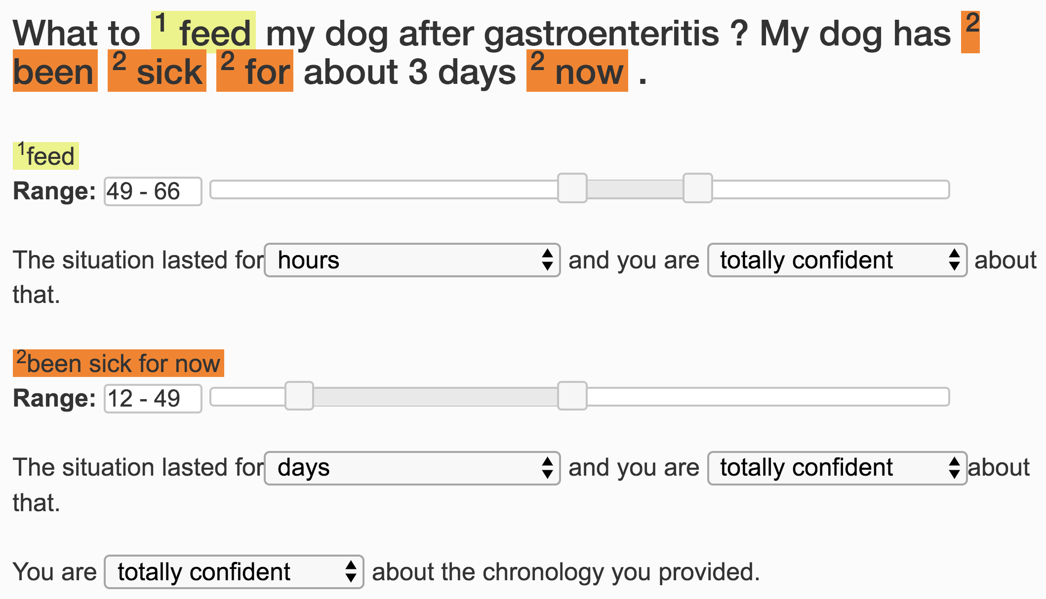 Figure 1
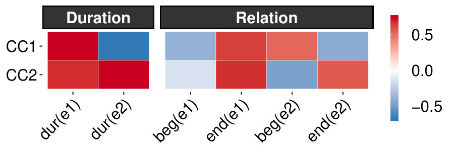 Figure 2
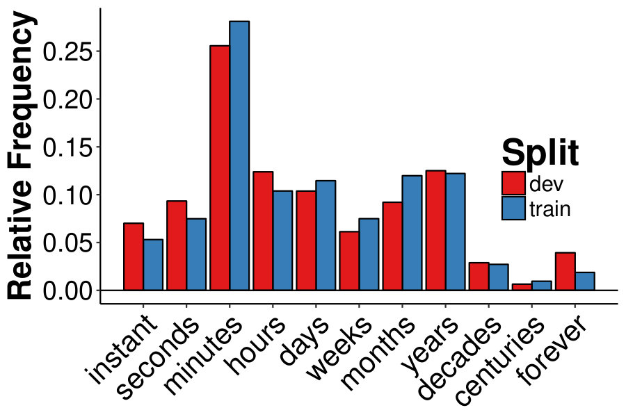 Figure 3
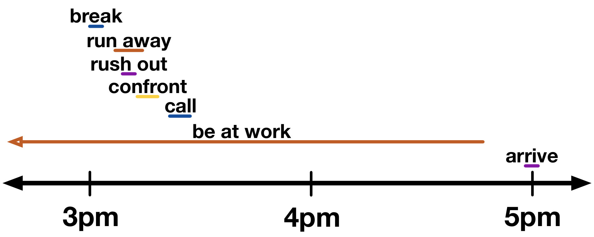 Figure 4
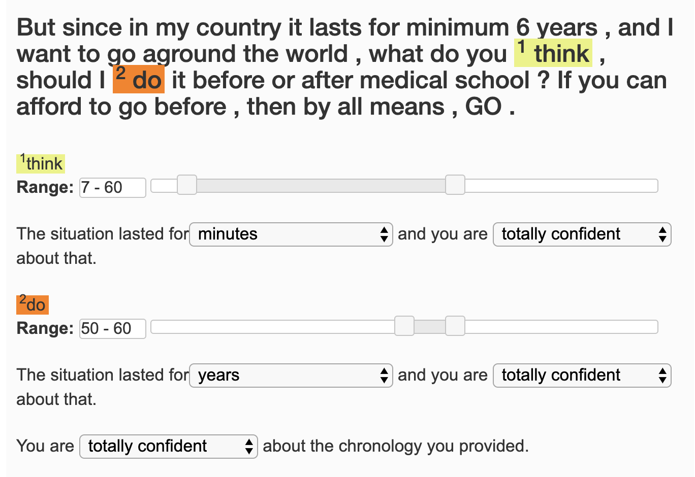 Figure 5
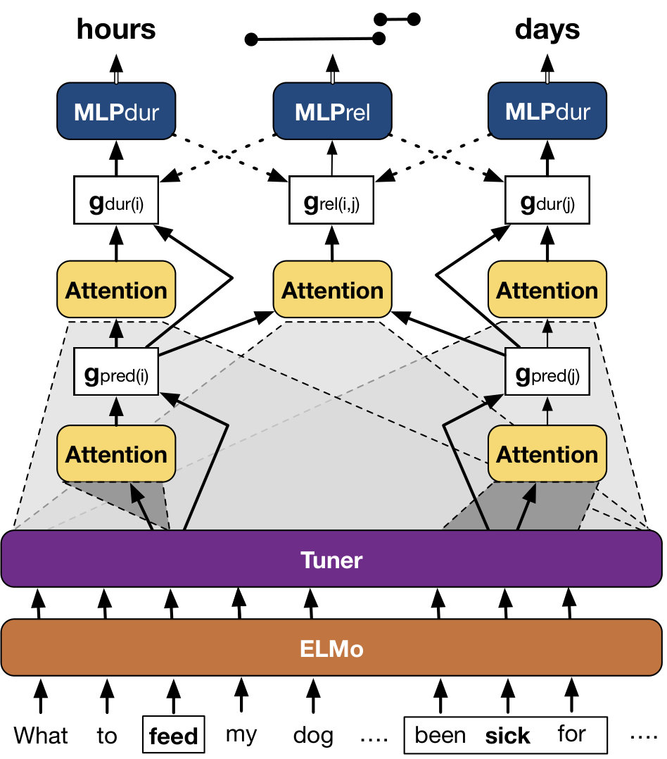 Figure 6
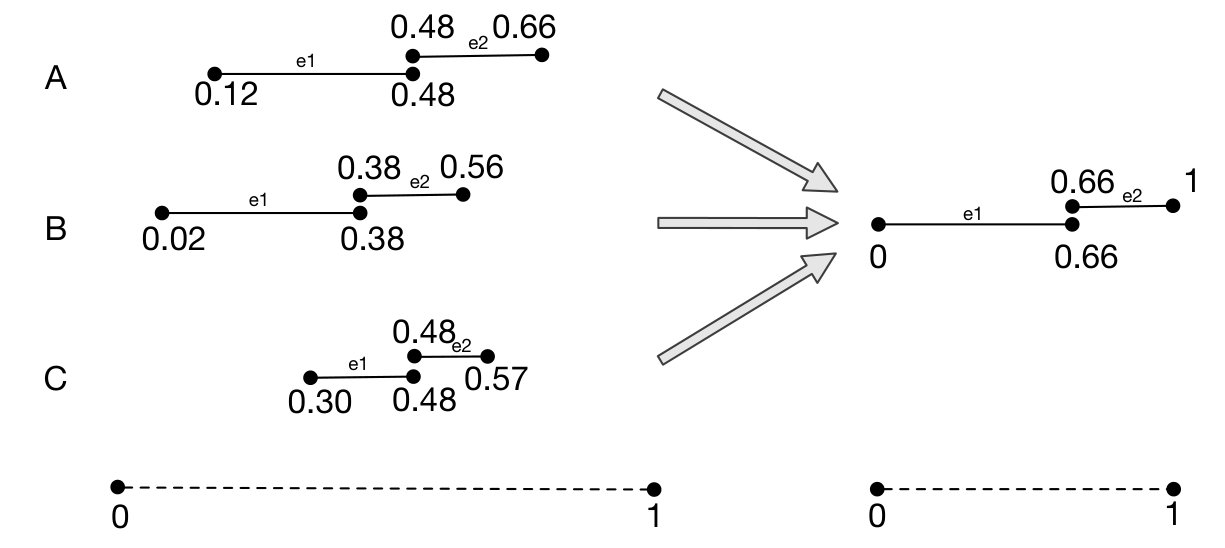 Figure 7
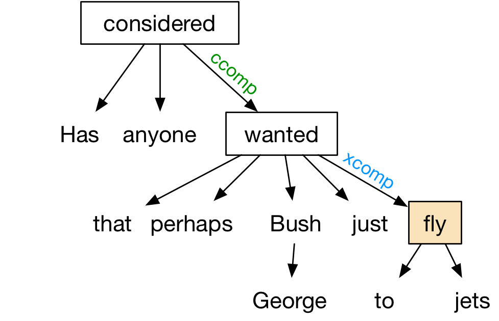 Figure 8
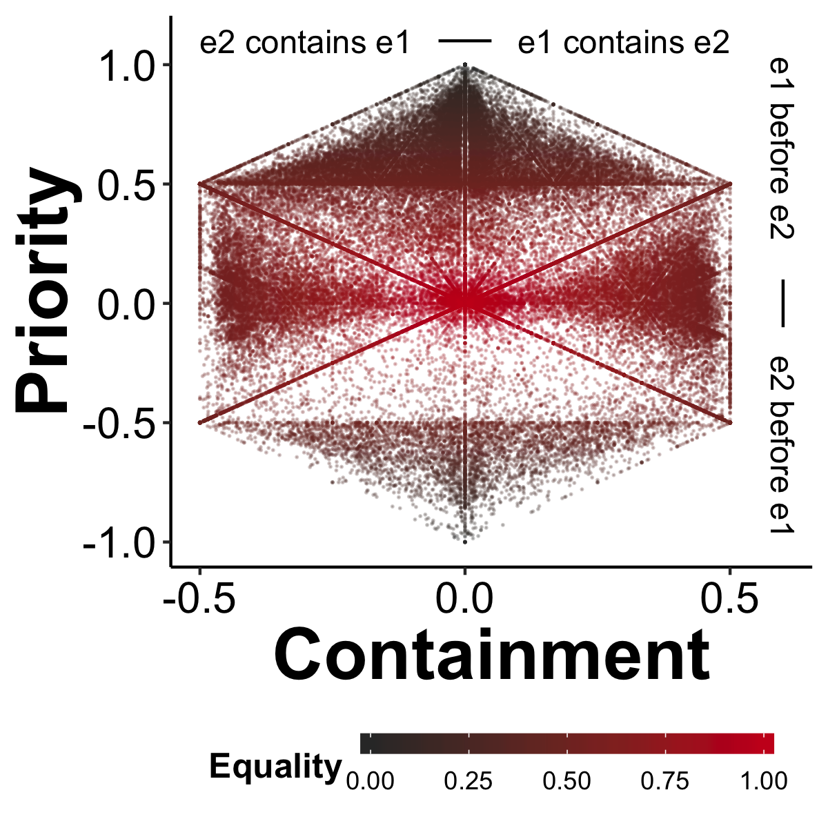 Figure 9
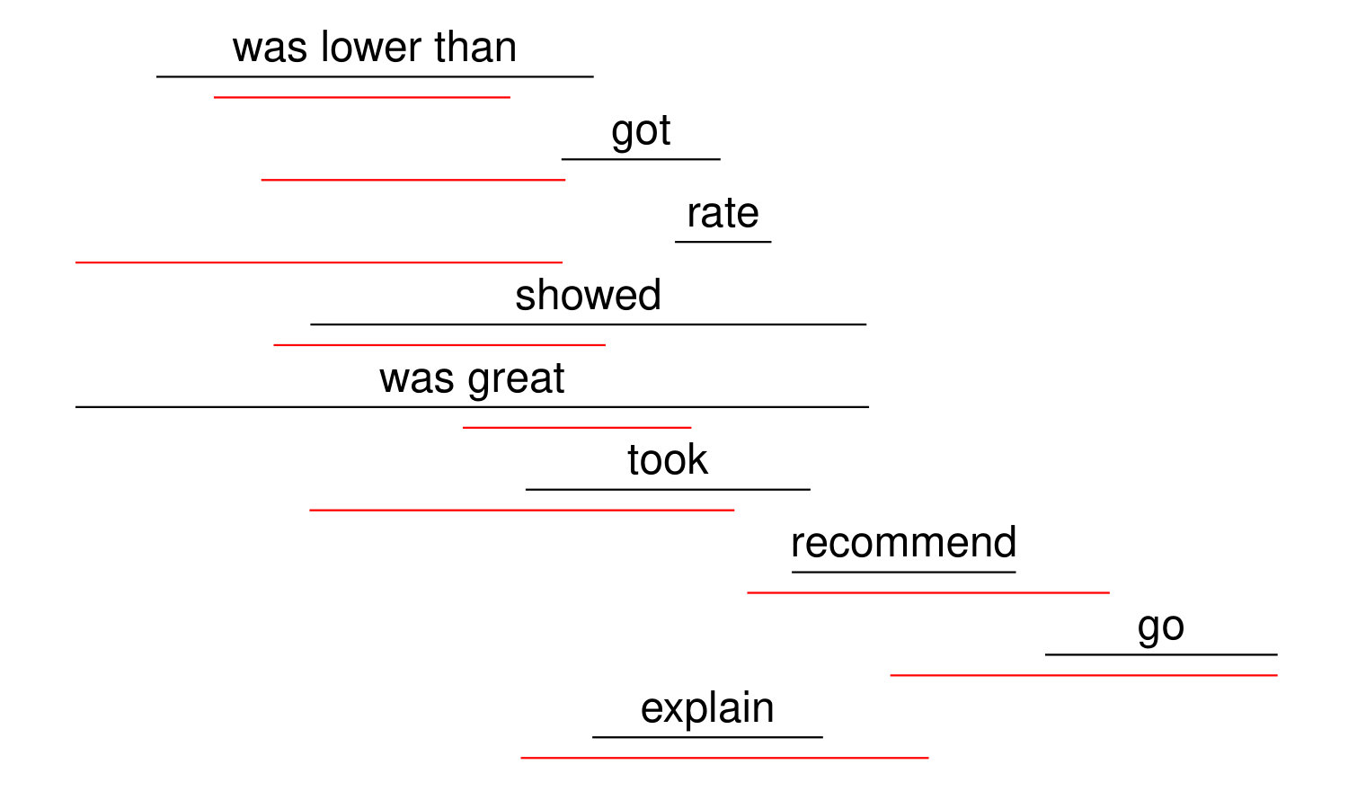 Figure 10
| Dataset | #Events | #Event-Event Relations |
|---|---|---|
| TimeBank | 7,935 | 3,481 |
| TempEval 2010 | 5,688 | 3,308 |
| TempEval 2013 | 11,145 | 5,272 |
| TimeBank-Dense | 1,729 | 8,130 |
| Hong et al. (2016) | 863 | 25,610 |
| UDS-T | 32,302 | 70,368 |
| Model | Duration | Relation | ||||||
|---|---|---|---|---|---|---|---|---|
| Duration | Relation | Connection | rank diff. | R1 | Absolute | Relative | R1 | |
| softmax | ✓ | - | 32.63 | 1.86 | -8.59 | 77.91 | 68.00 | -2.82 |
| binomial | ✓ | - | 37.75 | 1.75 | -13.73 | 77.87 | 67.68 | -2.35 |
| - | ✓ | Dur Rel | 22.65 | 3.08 | -51.68 | 71.65 | 66.59 | -6.09 |
| binomial | - | Dur Rel | 36.52 | 1.76 | -13.17 | 77.58 | 66.36 | -0.85 |
| binomial | ✓ | Dur Rel | 38.38 | 1.75 | -13.85 | 77.82 | 67.73 | -2.58 |
| binomial | ✓ | Dur Rel | 38.12 | 1.75 | -13.68 | 78.12 | 68.22 | -2.96 |
|
|
||||||||||||||||||||||||||||||||||||||||||||||||||||||||||||||||||||||||||||||||||||||||||||||||||||||||||||||||||||||||||||||||||||||||
| Systems | Evaluation Data | F1 |
| (E-E) | ||
| CAEVO | TD-test | 0.494 |
| CATENA | TD-test | 0.519 |
| Cheng and Miyao (2017) | TD-test | 0.529 |
| This work | TD-test | 0.566 |
Peer Reviews
No public reviews on file for this paper yet. If you reviewed it on a platform where reviews are public (OpenReview, ICLR, NeurIPS, ICML), you can paste yours below so the community can read it here.
Videos
No videos yet. Explain this paper in a talk, walkthrough, or lecture? Add one.
Fine-Grained Temporal Relation Extraction
Siddharth Vashishtha
University of Rochester
&Benjamin Van Durme
Johns Hopkins University
&Aaron Steven White
University of Rochester
Abstract
We present a novel semantic framework for modeling temporal relations and event durations that maps pairs of events to real-valued scales. We use this framework to construct the largest temporal relations dataset to date, covering the entirety of the Universal Dependencies English Web Treebank. We use this dataset to train models for jointly predicting fine-grained temporal relations and event durations. We report strong results on our data and show the efficacy of a transfer-learning approach for predicting categorical relations.
1 Introduction
Natural languages provide a myriad of formal and lexical devices for conveying the temporal structure of complex events—e.g. tense, aspect, auxiliaries, adverbials, coordinators, subordinators, etc. Yet, these devices are generally insufficient for determining the fine-grained temporal structure of such events. Consider the narrative in 1.
\ex
. At 3pm, a boy broke his neighbor’s window. He was running away, when the neighbor rushed out to confront him. His parents were called but couldn’t arrive for two hours because they were still at work.
Most native English speakers would have little difficulty drawing a timeline for these events, likely producing something like that in Figure 1. But how do we know that the breaking, the running away, the confrontation, and the calling were short, while the parents being at work was not? And why should the first four be in sequence, with the last containing the others?
The answers to these questions likely involve a complex interplay between linguistic information, on the one hand, and common sense knowledge about events and their relationships, on the other (Minsky, 1975; Schank and Abelson, 1975; Lamport, 1978; Allen and Hayes, 1985; Hobbs et al., 1987; Hwang and Schubert, 1994). But it remains a question how best to capture this interaction.
A promising line of attack lies in the task of temporal relation extraction. Prior work in this domain has approached this task as a classification problem, labeling pairs of event-referring expressions—e.g. broke or be at work in 1—and time-referring expressions—e.g. 3pm or two hours—with categorical temporal relations (Pustejovsky et al., 2003; Styler IV et al., 2014; Minard et al., 2016). The downside of this approach is that time-referring expressions must be relied upon to express duration information. But as 1 highlights, nearly all temporal duration information can be left implicit without hindering comprehension, meaning these approaches only explicitly encode duration information when that information is linguistically realized.
In this paper, we develop a novel framework for temporal relation representation that puts event duration front and center. Like standard approaches using the TimeML standard, we draw inspiration from Allen’s (1983) seminal work on interval representations of time. But instead of annotating text for categorical temporal relations, we map events to their likely durations and event pairs directly to real-valued relative timelines. This change not only supports the goal of giving a more central role to event duration, it also allows us to better reason about the temporal structure of complex events as described by entire documents.
We first discuss prior work on temporal relation extraction (§2) and then present our framework and data collection methodology (§3). The resulting dataset—Universal Decompositional Semantics Time (UDS-T)—is the largest temporal relation dataset to date, covering all of the Universal Dependencies Silveira et al. (2014); De Marneffe et al. (2014); Nivre et al. (2015) English Web Treebank (Bies et al., 2012). We use this dataset to train a variety of neural models (§4) to jointly predict event durations and fine-grained (real-valued) temporal relations (§5), yielding not only strong results on our dataset, but also competitive performance on TimeML-based datasets (§6).111Data and code are available at http://decomp.io/.
2 Background
We review prior work on temporal relations frameworks and temporal relation extraction systems.
Corpora
Most large temporal relation datasets use the TimeML standard (Pustejovsky et al., 2003; Styler IV et al., 2014; Minard et al., 2016). TimeBank is one of the earliest large corpora built using this standard, aimed at capturing ‘salient’ temporal relations between events (Pustejovsky et al., 2003). The TempEval competitions build on TimeBank by covering relations between all the events and times in a sentence.
Inter-sentential relations, which are necessary for document-level reasoning, have not been a focus of the TempEval tasks, though at least one sub-task does address them (Verhagen et al., 2007, 2010; UzZaman et al., 2013, and see Chambers et al. 2014). Part of this likely has to do with the sparsity inherent in the TempEval event-graphs. This sparsity has been addressed with corpora such as the TimeBank-Dense, where annotators label all local-edges irrespective of ambiguity (Cassidy et al., 2014). TimeBank-Dense does not capture the complete graph over event and time relations, instead attempting to achieve completeness by capturing all relations both within a sentence and between neighboring sentences. We take inspiration from this work for our own framework.
This line of work has been further improved on by frameworks such as Richer Event Description (RED), which uses a multi-stage annotation pipeline where various event-event phenomena, including temporal relations and sub-event relations are annotated together in the same datasets (O’Gorman et al., 2016). Similarly, Hong et al. (2016) build a cross-document event corpus which covers fine-grained event-event relations and roles with more number of event types and sub-types (see also Fokkens et al., 2013).
Models
Early systems for temporal relation extraction use hand-tagged features modeled with multinomial logistic regression and support vector machines (Mani et al., 2006; Bethard, 2013; Lin et al., 2015). Other approaches use combined rule-based and learning-based approaches (D’Souza and Ng, 2013) and sieve-based architectures—e.g. CAEVO (Chambers et al., 2014) and CATENA (Mirza and Tonelli, 2016). Recently, Ning et al. (2017) use a structured learning approach and show significant improvements on both TempEval-3 (UzZaman et al., 2013) and TimeBank-Dense (Cassidy et al., 2014). Ning et al. (2018) show further improvements on TimeBank-Dense by jointly modeling causal and temporal relations using Constrained Conditional Models and formulating the problem as an Interger Linear Programming problem.
Neural network-based approaches have used both recurrent (Tourille et al., 2017; Cheng and Miyao, 2017; Leeuwenberg and Moens, 2018) and convolutional architectures (Dligach et al., 2017). Such models have furthermore been used to construct document timelines from a set of predicted temporal relations (Leeuwenberg and Moens, 2018). Such use of pairwise annotations can result in inconsistent temporal graphs, and efforts have been made to avert this issue by employing temporal reasoning (Chambers and Jurafsky, 2008; Yoshikawa et al., 2009; Denis and Muller, 2011; Do et al., 2012; Laokulrat et al., 2016; Ning et al., 2017; Leeuwenberg and Moens, 2017).
Other work has aimed at modeling event durations from text (Pan et al., 2007; Gusev et al., 2011; Williams and Katz, 2012), though this work does not tie duration to temporal relations (see also Filatova and Hovy, 2001). Our approach combines duration and temporal relation information within a unified framework, discussed below.
3 Data Collection
We collect the Universal Decompositional Semantics Time (UDS-T) dataset, which is annotated on top of the Universal Dependencies Silveira et al. (2014); De Marneffe et al. (2014); Nivre et al. (2015) English Web Treebank (Bies et al., 2012) (UD-EWT). The main advantages of UD-EWT over other similar corpora are: (i) it covers text from a variety of genres; (ii) it contains gold standard Universal Dependency parses; and (iii) it is compatible with various other semantic annotations which use the same predicate extraction standard White et al. (2016); Zhang et al. (2017); Rudinger et al. (2018); Govindarajan et al. (2019). Table 1 compares the size of UDS-T against other temporal relations datasets.
Protocol design
Annotators are given two contiguous sentences from a document with two highlighted event-referring expressions (predicates). They are then asked (i) to provide relative timelines on a bounded scale for the pair of events referred to by the highlighted predicates; and (ii) to give the likely duration of the event referred to by the predicate from the following list: instantaneous, seconds, minutes, hours, days, weeks, months, years, decades, centuries, forever. In addition, annotators were asked to give a confidence ratings for their relation annotation and each of their two duration annotation on the same five-point scale - not at all confident (0), not very confident (1), somewhat confident (2), very confident (3), totally confident (4).
An example of the annotation instrument is shown in Figure 2. Henceforth, we refer to the situation referred to by the predicate that comes first in linear order (feed in Figure 2) as and the situation referred to by the predicate that comes second in linear order (sick in Figure 2) as .
Annotators
We recruited 765 annotators from Amazon Mechanical Turk to annotate predicate pairs in groups of five. Each predicate pair contained in the UD-EWT train set was annotated by a single annotator, and each in the UD-EWT development and test sets was annotated by three.
Predicate extraction
We extract predicates from UD-EWT using PredPatt White et al. (2016); Zhang et al. (2017), which identifies 33,935 predicates from 16,622 sentences. We concatenate all pairs of adjacent sentences in the documents contained in UD-EWT, allowing us to capture inter-sentential temporal relations. Considering all possible pairs of predicates in adjacent sentences is infeasible, so we use a heuristic to capture the most interesting pairs. (See Appendix A for details.)
Normalization
We normalize the slider responses for each event pair by subtracting the minimum slider value from all values, then dividing all such shifted values by the maximum value (after shifting). This ensures that the earliest beginning point for every event pair lies at 0 and that the right-most end-point lies at 1 while preserving the ratio between the durations implied by the sliders. Figure 3 illustrates this procedure for three hypothetical annotators annotating the same two events and . Assuming that the duration classes for or do not differ across annotators, the relative chronology of the events is the same in each case. This preservation of relative chronology, over absolute slider position, is important because, for the purposes of determining temporal relation, the absolute positions that annotators give are meaningless, and we do not want our models to be forced to fit to such irrelevant information.
Inter-annotator agreement
We measure inter-annotator agreement (IAA) for the temporal relation sliders by calculating the rank (Spearman) correlation between the normalized slider positions for each pair of annotators that annotated the same group of five predicate pairs in the development set.222Our protocol design also allows us to detect some bad annotations internal to the annotation itself, as opposed to comparing one annotator’s annotation of an item to another. See Appendix B for further details on our deployment of such annotation-internal validation techniques. The development set is annotated by 724 annotators. Rank correlation is a useful measure because it tells us how much different annotators agree of the relative position of each slider. The average rank correlation between annotators was 0.665 (95% CI=[0.661, 0.669]).
For the duration responses, we compute the absolute difference in duration rank between the duration responses for each pair of annotators that annotated the same group of five predicate pairs in the development set. On average, annotators disagree by 2.24 scale points (95% CI=[2.21, 2.25]), though there is heavy positive skew ( = 1.16, 95% CI=[1.15, 1.18])—evidenced by the fact that the modal rank difference is 1 (25.3% of the response pairs), with rank difference 0 as the next most likely (24.6%) and rank difference 2 as a distant third (15.4%).
Summary statistics
Figure 4 shows the distribution of duration responses in the training and development sets. There is a relatively high density of events lasting minutes, with a relatively even distribution across durations of years or less and few events lasting decades or more.
The raw slider positions themselves are somewhat difficult to directly interpret. To improve interpretability, we rotate the slider position space to construct four new dimensions: (i) priority, which is positive when starts and/or ends earlier than and negative otherwise; (ii) containment,which is most positive when contains more of ; (iii) equality, which is largest when both and have the same temporal extents and smallest when they are most unequal; and (iv) shift, which moves the events forward or backward in time. We construct these dimensions by solving for in
[TABLE]
where contains the slider positions for our datapoints in the following order: beg(), end(), beg(), end().
Figure 5 shows the embedding of the event pairs on the first three of these dimensions of . The triangular pattern near the top and bottom of the plot arises because strict priority—i.e. extreme positivity or negativity on the -axis—precludes any temporal overlap between the two events, and as we move toward the center of the plot, different priority relations mix with different overlap relations—e.g. the upper-middle left corresponds to event pairs where most of comes toward the beginning of , while the upper middle right of the plot corresponds to event pairs where most of comes toward the end of .
4 Model
For each pair of events referred to in a sentence, we aim to jointly predict the relative timelines of those events as well as their durations. We then use a separate model to induce document timelines from the relative timelines.
Relative timelines
The relative timeline model consists of three components: an event model, a duration model, and a relation model. These components use multiple layers of dot product attention (Luong et al., 2015) on top of an embedding for a sentence tuned on the three -dimensional contextual embeddings produced by ELMo (Peters et al., 2018) for that sentence, concatenated together.
[TABLE]
where is the dimension for the tuned embeddings, , and .
Event model
We define the model’s representation for the event referred to by predicate as \mathbf{g}_{\text{pred{}_{k}}}\in\mathbb{R}^{D}, where is the embedding size. We build this representation using a variant of dot-product attention, based on the predicate root.
[TABLE]
where ; \mathbf{h}_{\text{{root}(pred{}{k})}} is the hidden representation of the predicate’s root; and \mathbf{H}_{\text{{span}(pred{}{k})}} is obtained by stacking the hidden representations of the entire predicate.
As an example, the predicate been sick for now in Figure 2 has sick as its root, and thus we would take the hidden representation for sick as \mathbf{h}_{\text{{root}(pred{}{k})}}. Similarly, \mathbf{H}_{\text{{span}(pred{}{k})}} would be equal to taking the hidden-state representations of been sick for now and stacking them together. Then, if the model learns that tense information is important, it may weight been using attention.
Duration model
The temporal duration representation \mathbf{g}_{\text{dur{}_{k}}} for the event referred to by the predicate is defined similarly to the event representation, but instead of stacking the predicate’s span, we stack the hidden representations of the entire sentence .
[TABLE]
where \mathbf{A}^{\text{\sc sent}}_{\text{\sc dur}}\in\mathbb{R}^{D\times\text{size}(g_{\text{pred{}_{k}}})} and .
We consider two models of the categorical durations: a softmax model and a binomial model. The main difference is that the binomial model enforces that the probabilities \mathbf{p}_{\text{dur{}_{k}}} over the 11 duration values be concave in the duration rank, whereas the softmax model has no such constraint. We employ a cross-entropy loss for both models.
[TABLE]
In the softmax model, we pass the duration representation \mathbf{g}_{\text{dur{}{k}}} for predicate through a multilayer perceptron (MLP) with a single hidden layer of ReLU activations, to yield probabilities \mathbf{p}_{\text{dur{}{k}}} over the 11 durations.
[TABLE]
In the binomial distribution model, we again pass the duration representation through a MLP with a single hidden layer of ReLU activations, but in this case, we yield only a single value \pi_{\text{dur{}{k}}}. With \mathbf{v}_{\text{dur{}{k}}} as defined above:
[TABLE]
where represents the ranked durations – instant (0), seconds (1), minutes (2), …, centuries (9), forever (10) – and is the maximum class rank (10).
Relation model
To represent the temporal relation representation between the events referred to by the and predicate, we again use a similar attention mechanism.
[TABLE]
where \mathbf{A}^{\text{\sc sent}}_{\text{\sc rel}}\in\mathbb{R}^{D\times 2\text{size}(g_{\text{pred{}_{k}}})} and .
The main idea behind our temporal model is to map events and states directly to a timeline, which we represent via a reference interval . For situation , we aim to predict the beginning point bk and end-point \text{e{}{k}}\geq\text{b{}{k}} of .
We predict these values by passing through an MLP with one hidden layer of ReLU activations and four real-valued outputs , representing the estimated relative beginning points () and durations () for events and . We then calculate the predicted slider values
[TABLE]
The predicted values are then normalized in the same fashion as the true slider values prior to being entered into the loss. We constrain this normalized using four L1 losses.
[TABLE]
The final loss function is then .
Duration-relation connections
We also experiment with four architectures wherein the duration and relation models are connected to each other in the Dur Rel or Dur Rel directions.
In the Dur Rel architectures, we modify in two ways: (i) additionally concatenating the and predicate’s duration probabilities from the binomial distribution model, and (ii) not using the relation representation model at all.
[TABLE]
In the Dur Rel architectures, we use two modifications: (i) we modify by concatenating the and from the relation model, and (ii) we do not use the duration representation model at all, instead use the predicted relative duration obtained from the relation model, passing it through the binomial distribution model.
[TABLE]
Document timelines
We induce the hidden document timelines for the documents in the UDS-T development set using relative timelines from (i) actual pairwise slider annotations; or (ii) slider values predicted by the best performing model on UDS-T development set. To do this, we assume a hidden timeline , where is the total number of predicates in that document, the two dimensions represent the beginning point and the duration of the predicates. We connect these latent timelines to the relative timelines, by anchoring the beginning points of all predicates such that there is always a predicate with 0 as the beginning point in a document and defining auxiliar variables and for each events and .
[TABLE]
We learn for each document under the relation loss . We further constrain to predict the categorical durations using the binomial distribution model on the durations implied by , assuming .
5 Experiments
We implement all models in pytorch 1.0. For all experiments, we use mini-batch gradient descent with batch-size 64 to train the embedding tuner (reducing ELMo to a dimension of 256), attention, and MLP parameters. Both the relation and duration MLP have a single hidden layer with 128 nodes and a dropout probability of 0.5 (see Appendix D for further details).
To predict TimeML relations in TempEval3 (TE3; UzZaman et al., 2013, Task C-relation only) and TimeBank-Dense (TD; Cassidy et al., 2014), we use a transfer learning approach. We first use the best-performing model on the UDS-T development set to obtain the relation representation () for each pair of annotated event-event relations in TE3 and TD (see Appendix E for preprocessing details). We then use this vector as input features to a SVM classifier with a Gaussian kernel to train on the training sets of these datasets using the feature vector obtained from our model.333For training on TE3, we use TimeBank (TB; Pustejovsky et al., 2003) + AQUAINT (AQ; Graff, ) datasets provided in the TE3 workshop (UzZaman et al., 2013). For training on TD, we use TD-train and TD-dev.
Following recent work using continuous labels in event factuality prediction Lee et al. (2015); Stanovsky et al. (2017); Rudinger et al. (2018); White et al. (2018) and genericity prediction Govindarajan et al. (2019), we report three metrics for the duration prediction: Spearman correlation (), mean rank difference (rank diff), and proportion rank difference explained (R1). We report three metrics for the relation prediction: Spearman correlation between the normalized values of actual beginning and end points and the predicted ones (absolute ), the Spearman correlation between the actual and predicted values in (relative ), and the proportion of MAE explained (R1).
[TABLE]
where is always guessing the median.
6 Results
Table 2 shows the results of different model architectures on the UDS-T test set, and Table 4 shows the results of our transfer-learning approach on test set of TimeBank-Dense (TD-test).
UDS-T results
Most of our models are able to predict the relative position of the beginning and ending of events very well (high relation ) and the relative duration of events somewhat well (relatively low duration ), but they have a lot more trouble predicting relation exactly and relatively less trouble predicting duration exactly.
Duration model
The binomial distribution model outperforms the softmax model for duration prediction by a large margin, though it has basically no effect on the accuracy of the relation model, with the binomial and softmax models performing comparably. This suggests that enforcing concavity in duration rank on the duration probabilities helps the model better predict durations.
Connections
Connecting the duration and relation model does not improve performance in general. In fact, when the durations are directly predicted from the temporal relation model—i.e. without using the duration representation model—the model’s performance drops by a large margin, with the Spearman correlation down by roughly 15 percentage points. This indicates that constraining the relations model to predict the durations is not enough and that the duration representation is needed to predict durations well. On the other hand, predicting temporal relations directly from the duration probability distribution—i.e. without using the relation representation model—results in a similar score as that of the top-performing model. This indicates that the duration representation is able to capture most of the relation characteristics of the sentence. Using both duration representation and relation representation separately (model highlighted in blue) results in the best performance overall on the UDS-T development set.
TimeBank-Dense and TempEval3
Table 4 reports F1-micro scores on the test set of TimeBank-Dense compared with some other systems as reported by Cheng and Miyao (2017). We report these scores only on Event-Event (E-E) relations as our system captures only those. We also compute the standard temporal awareness F1 score on the test set of TempEval-3 (TE3-PT) considering only E-E relations and achieve a score of 0.498.444We do not report the temporal awareness scores (F1) of other systems on TE3-PT, since they report their metrics on all relations, including timex-timex, and event-timex relations, and thus they are not directly comparable. For TD, only those systems are reported that report F1-micro scores. Our system beats the TD F1-micro scores of all other systems reported in Table 4. As a reference, the top performing system on TE3-PT (Ning et al., 2017) reports an F1 score of 0.672 over all relations, but is not directly comparable to our system as we only evaluate on event-event relations. These results indicate that our model is able to achieve competitive performance on other standard temporal classification problems.
7 Model Analysis and Timelines
We investigate two aspects of the best-performing model on the development set (highlighted in Table 2): (i) what our duration and relation representations attend to; and (ii) how well document timelines constructed from the model’s predictions match those constructed from the annotations. (See Appendix F for further analyses.)
Attention
The advantage of using an attention mechanism is that we can often interpret what linguistic information the model is using by analyzing the attention weights. We extract these attention weights for both the duration representation and the relation representation from our best model on the development set.
Duration
We find that words that denote some time period—e.g. month(s), minutes, hour, years, days, week—are among the words with highest mean attention weight in the duration model, with seven of the top 15 words directly denoting one of the duration classes (Table 3). This is exactly what one might expect this model to rely heavily on, since time expressions are likely highly informative for making predictions about duration. It also may suggest that we do not need to directly encode relations between event-referring and time-referring expressions in our framework—as do annotation standards like TimeML—since our models may discover them.
The remainder of the top words in the duration model are plurals or mass nouns (soldiers, thoughts etc.). This may suggest that the plurality of a predicate’s arguments is an indicator of the likely duration of the event referred to by that predicate. To investigate this possibility, we compute a multinomial regression predicting the attention weights for each sentence from the morphological features of each word in that sentence , which are extracted from the UD-EWT features column and binarized. To do this, we optimize coefficients in , where is the KL divergence. We find that the five most strongly weighted positive features in are all features of nouns—number=plur, case=acc, prontype=prs, number=sing, gender=masc—suggesting that good portion of duration information can be gleaned from the arguments of a predicate. This may be because nominal information can be useful in determining whether the clause is about particular events or generic events Govindarajan et al. (2019).
Relation
A majority of the words with highest mean attention weight in the relation model are either coordinators—such as or and and—or bearers of tense information—i.e. lexical verbs and auxiliaries. The first makes sense because, in context, coordinators can carry information about temporal sequencing (see Wilson and Sperber, 1998, i.a.). The second makes sense in that information about the tense of predicates being compared likely helps the model determine relative ordering of the events they refer to.
Similar to duration attention analysis, for relation attention, we find that the five most strongly weighted positive features in are all features of verbs or auxiliaries—person=1, person=3, tense=pres, tense=past, mood=ind—suggesting that a majority of the information relevant to relation can be gleaned from the tense-bearing units in a clause.
Document timelines
We apply the document timeline model described in §4 to both the annotations on the development set and the best-performing model’s predictions to obtain timelines for all documents in the development set. Figure 7 shows an example, comparing the two resulting document timelines.
For these two timelines, we compare the induced beginning points and durations, obtaining a mean Spearman correlation of 0.28 for beginning points and -0.097 for durations. This suggests that the model agrees to some extent with the annotations about the beginning points of events in most documents but is struggling to find the correct duration spans. One possible reason for poor prediction of durations could be the lack of a direct source of duration information. The model currently tries to identify the duration based only on the slider values, which leads to poor performance as already seen in one of the Dur Rel model.
8 Conclusion
We presented a novel semantic framework for modeling fine-grained temporal relations and event durations that maps pairs of events to real-valued scales for the purpose of constructing document-level event timelines. We used this framework to construct the largest temporal relations dataset to date – UDS-T – covering the entirety of the UD-EWT. We used this dataset to train models for jointly predicting fine-grained temporal relations and event durations, reporting strong results on our data and showing the efficacy of a transfer-learning approach for predicting standard, categorical TimeML relations.
Acknowledgments
We are grateful to the FACTS.lab at the University of Rochester as well as three anonymous reviewers for useful comments on this work. This research was supported by the University of Rochester, JHU HLTCOE, and DARPA AIDA. The U.S. Government is authorized to reproduce and distribute reprints for Governmental purposes. The views and conclusions contained in this publication are those of the authors and should not be interpreted as representing official policies or endorsements of DARPA or the U.S. Government.
Appendix A Data Collection
We concatenate two adjacent sentences to form a combined sentence which allows us to capture inter-sentential temporal relations. Considering all possible pairs of events in the combined sentence results into an exploding number of event-event comparisons. Therefore, to reduce the total number of comparisons, we find the pivot-predicate of the antecedent of the combined sentence as follows - find the root predicate of the antecedent and if it governs a CCOMP, CSUBJ, or XCOMP, follow that dependency to the next predicate until a predicate is found that doesn’t govern a CCOMP, CSUBJ, or XCOMP. We then take all pairs of the antecedent predicates and pair every predicate of the consequent only with the pivot-predicate. This results into predicates instead of per sentence, where N and M are the number of predicates in the antecedent and consequent respectively. This heuristic allows us to find a predicate that loosely denotes the topic being talked about in the sentence. Figure 8 shows an example of finding the pivot predicate.
Appendix B Rejecting Annotations
We design multiple checks to detect potentially bad annotations during our data collection. A single assignment contains 5 annotations (predicate-pairs). Once an annotation is flagged by any of these checks, we may accept or reject the assignment based on our subjective opinion about the particular case. Annotations are flagged based on the following conditions:
B.1 Time completion
Our pilot studies indicate a median time of roughly 4 minutes to complete a single assignment (5 annotations). We automatically reject any assignment which is completed under a minute as we believe that it is not plausible to finish the assignment within a minute. We find that such annotations mostly had default values annotated.
B.2 Same slider values
If all the beginning points and end-points in an assignment have the same values, we automatically reject those assignments.
B.3 Same duration values
Sometimes we encounter cases where all duration values in an assignment are annotated to have the same value. This scenario , although unlikely, could genuinely be an instance of correct annotation. Hence we manually check for these cases and reject only if the annotations look dubious in nature based on our subjective opinion.
B.4 Inconsistency between the slider positions and durations
Our protocol design allows us to detect potentially bad annotations by detecting inconsistency between the slider positions (beginning and end-points) and the duration values of events in an annotated sentence. The annotator in Figure 9 assigns slider values for (think) as [7,60] i.e. a time-span of 53 and assigns its duration as minutes. But at the same time, the slider values for (do) are annotated as [50,60] i.e. a time-span of 10, even though its duration is assigned as years. This is an inconsistency as has a smaller time-span denoted by the sliders but has the longer duration as denoted by years. We reject assignments where more than 60% of annotations have this inconsistency.
Appendix C Inter-annotator agreement
Annotators were asked to approximate the relative duration of the two events that they were annotating using the distance between the sliders. This means that an annotation is coherent insofar as the ratio of distances between the slider responses for each event matches the ratio of the categorical duration responses. We rejected annotations wherein there was gross mismatch between the categorical responses and the slider responses — i.e. one event is annotated as having a longer duration but is given a shorter slider response — but because this does not guarantee that the exact ratios are preserved, we assess that here using a canonical correlation analysis (CCA; Hotelling 1936) between the categorical duration responses and the slider responses.
Figure 10 shows the CCA scores. We find that the first canonical correlation, which captures the ratios between unequal events, is 0.765; and the second, which captures the ratios between roughly unequal events, is 0.427. This preservation of the ratios is quite impressive in light of the fact that our slider scales are bounded; though we hoped for at least a non-linear relationship between the categorical durations and the slider distances, we did not expect such a strong linear relationship.
Appendix D Confidence Ratings
Annotators use the confidence scale in different ways. Some always respond with totally confident whereas others use all five options. To cater to these differences, we normalize the confidence ratings for each event-pair using a standard ordinal scale normalization technique known as ridit scoring. In ridit scoring ordinal labels are mapped to (0, 1) using the empirical cumulative distribution function of the ratings given by each annotator. Ridit scoring re-weights the importance of a scale label based on the frequency of its usage.
We weight both , and by the ridit-scored confidence ratings of event durations and event relations, respectively.
Appendix E Processing TempEval3 and TimeBank-Dense
Since we require spans of predicates for our model, we pre-process TB+AQ and TD by removing all xml tags from the sentences and then we pass it through Stanford CoreNLP 3.9.2 (Manning et al., 2014) to get the corresponding conllu format. Roots and spans of predicates are then extracted using PredPatt. To train the SVM classifier, we use sklearn 0.20.0; Pedregosa et al. 2011. We run a hyperparameter grid-search over 4-fold CV with C: (0.1, 1, 10), and gamma: (0.001, 0.01, 0.1, 1). The best performance on cross-validation (C=1 and gamma=0.001) is then evaluated on the test set of TE3 i.e. TE3-Platinum (TE3-PT), and TD-test. For our purposes, the identity and simultaneous relations in TB+AQ are equivalent when comparing event-event relations. Hence, they are collapsed into one single relation.
Appendix F Further analysis
We rotate the predicted slider positions in the relation space defined in §3 and compare it with the rotated space of actual slider positions. We see a Spearman correlation of 0.19 for priority, 0.23 for containment, and 0.17 for equality. This suggests that our model is best able to capture containment relations and slightly less good at capturing priority and equality relations, though all the numbers are quite low compared to the absolute and relative metrics reported in Table 2. This may be indicative of the fact that our models do somewhat poorly on predicting more fine-grained aspects of an event relation, and in the future it may be useful to jointly train against the more interpretable priority, containment, and equality measures instead of or in conjunction with the slider values.
The reference list from the paper itself. Each links out to its DOI / PubMed record.
- 1Allen (1983) James F Allen. 1983. Maintaining knowledge about temporal intervals. Communications of the ACM , 26(11):832–843.
- 2Allen and Hayes (1985) James F Allen and Patrick J Hayes. 1985. A common-sense theory of time. In Proceedings of the 9th International Joint Conference on Artificial Intelligence-Volume 1 , pages 528–531. Morgan Kaufmann Publishers Inc.
- 3Bethard (2013) Steven Bethard. 2013. Cleartk-timeml: A minimalist approach to tempeval 2013. In Second Joint Conference on Lexical and Computational Semantics (* SEM), Volume 2: Proceedings of the Seventh International Workshop on Semantic Evaluation (Sem Eval 2013) , volume 2, pages 10–14.
- 4Bies et al. (2012) Ann Bies, Justin Mott, Colin Warner, and Seth Kulick. 2012. English web treebank. Linguistic Data Consortium, Philadelphia, PA .
- 5Cassidy et al. (2014) Taylor Cassidy, Bill Mc Dowell, Nathanael Chambers, and Steven Bethard. 2014. An annotation framework for dense event ordering. In Proceedings of the 52nd Annual Meeting of the Association for Computational Linguistics (Volume 2: Short Papers) , volume 2, pages 501–506.
- 6Chambers et al. (2014) Nathanael Chambers, Taylor Cassidy, Bill Mc Dowell, and Steven Bethard. 2014. Dense event ordering with a multi-pass architecture. Transactions of the Association for Computational Linguistics , 2:273–284.
- 7Chambers and Jurafsky (2008) Nathanael Chambers and Dan Jurafsky. 2008. Jointly combining implicit constraints improves temporal ordering. In Proceedings of the Conference on Empirical Methods in Natural Language Processing , pages 698–706. Association for Computational Linguistics.
- 8Cheng and Miyao (2017) Fei Cheng and Yusuke Miyao. 2017. Classifying temporal relations by bidirectional lstm over dependency paths. In Proceedings of the 55th Annual Meeting of the Association for Computational Linguistics (Volume 2: Short Papers) , volume 2, pages 1–6.