TL;DR
This paper introduces a machine learning-based method for efficiently estimating information leakage in black-box systems, especially those with large or continuous output spaces, improving over traditional frequency-based approaches.
Contribution
It proposes using universally consistent ML rules, particularly nearest neighbor methods, to accurately estimate leakage with fewer queries and applicability to continuous outputs.
Findings
ML-based methods reduce the number of queries needed
Nearest neighbor rules handle continuous output systems
Compared favorably with state-of-the-art leakage estimation tools
Abstract
We consider the problem of measuring how much a system reveals about its secret inputs. We work under the black-box setting: we assume no prior knowledge of the system's internals, and we run the system for choices of secrets and measure its leakage from the respective outputs. Our goal is to estimate the Bayes risk, from which one can derive some of the most popular leakage measures (e.g., min-entropy, additive, and multiplicative leakage). The state-of-the-art method for estimating these leakage measures is the frequentist paradigm, which approximates the system's internals by looking at the frequencies of its inputs and outputs. Unfortunately, this does not scale for systems with large output spaces, where it would require too many input-output examples. Consequently, it also cannot be applied to systems with continuous outputs (e.g., time side channels, network traffic). In this…
Click any figure to enlarge with its caption.
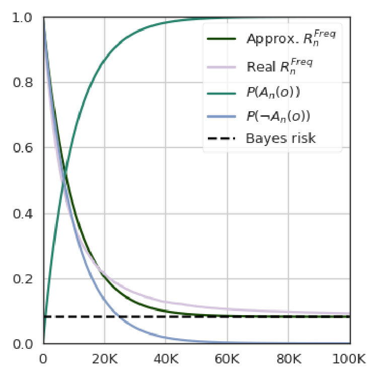 Figure 1
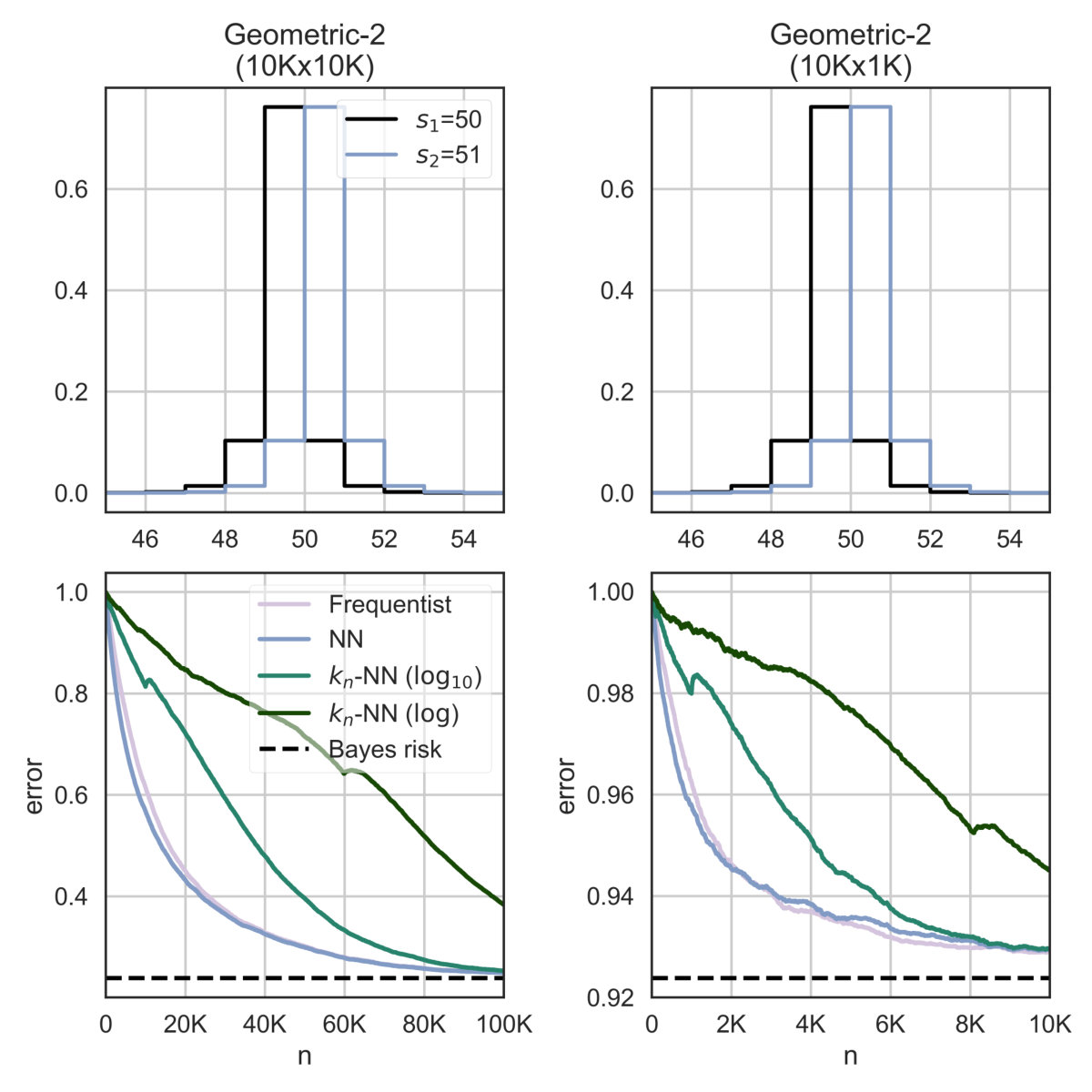 Figure 2
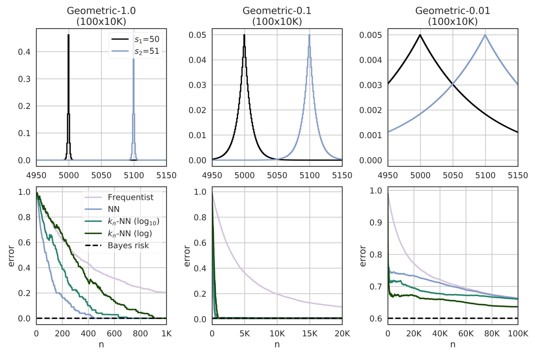 Figure 3
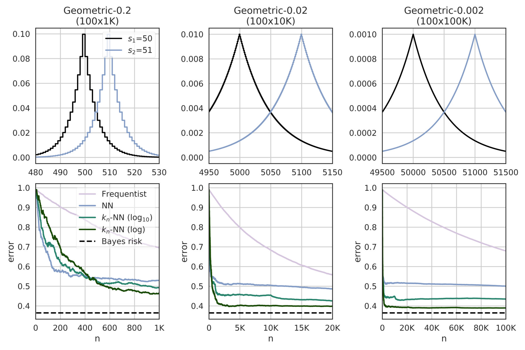 Figure 4
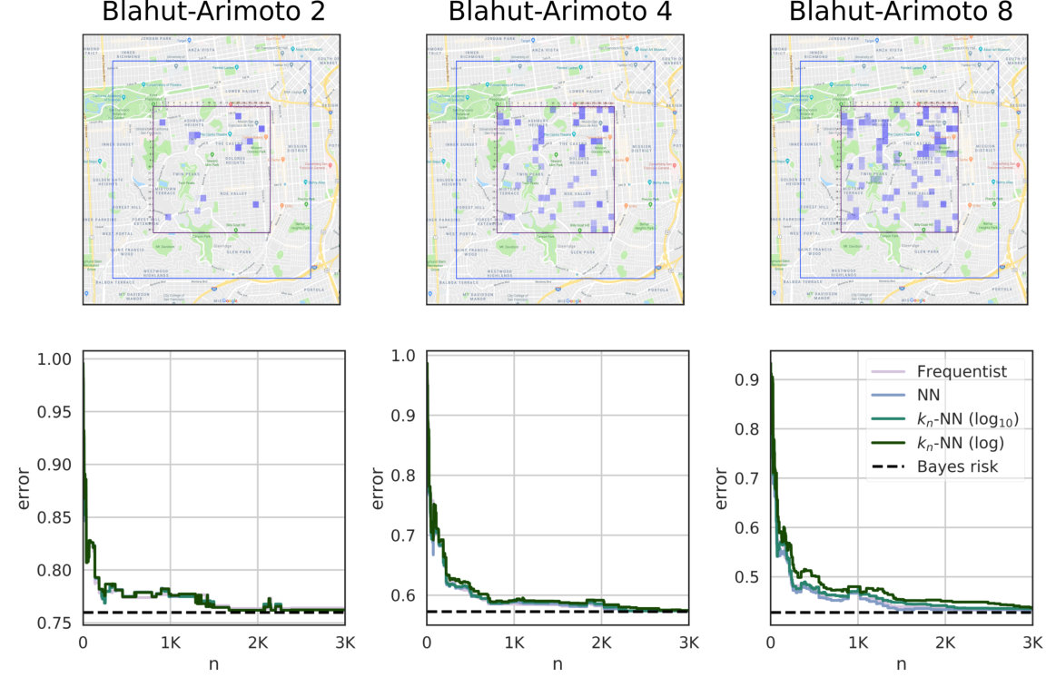 Figure 5
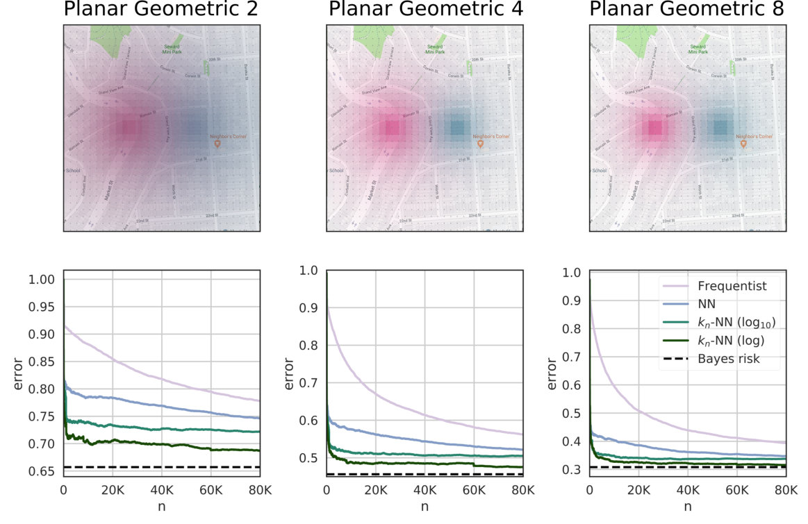 Figure 6
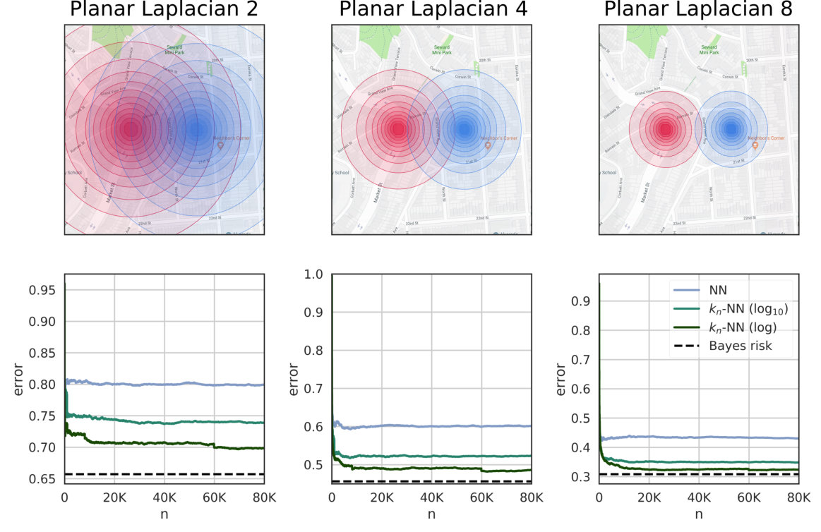 Figure 7
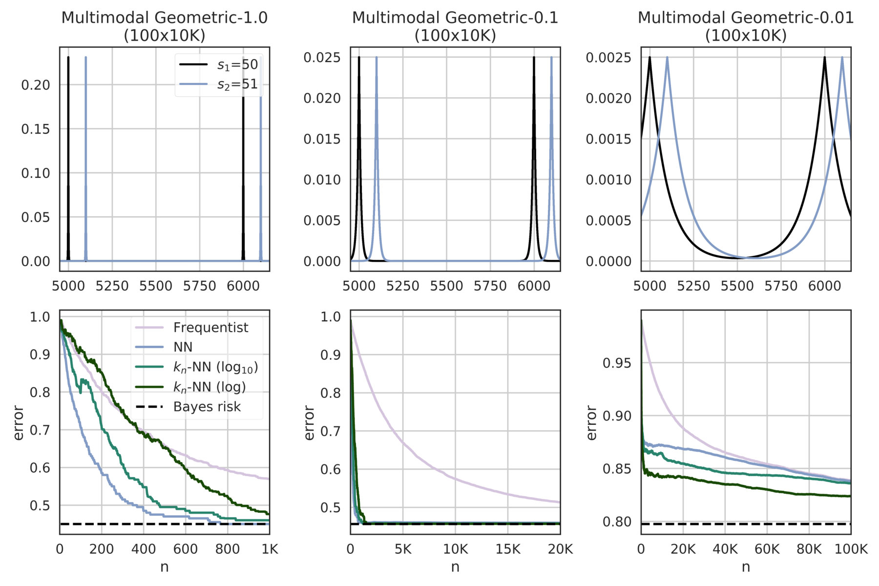 Figure 8
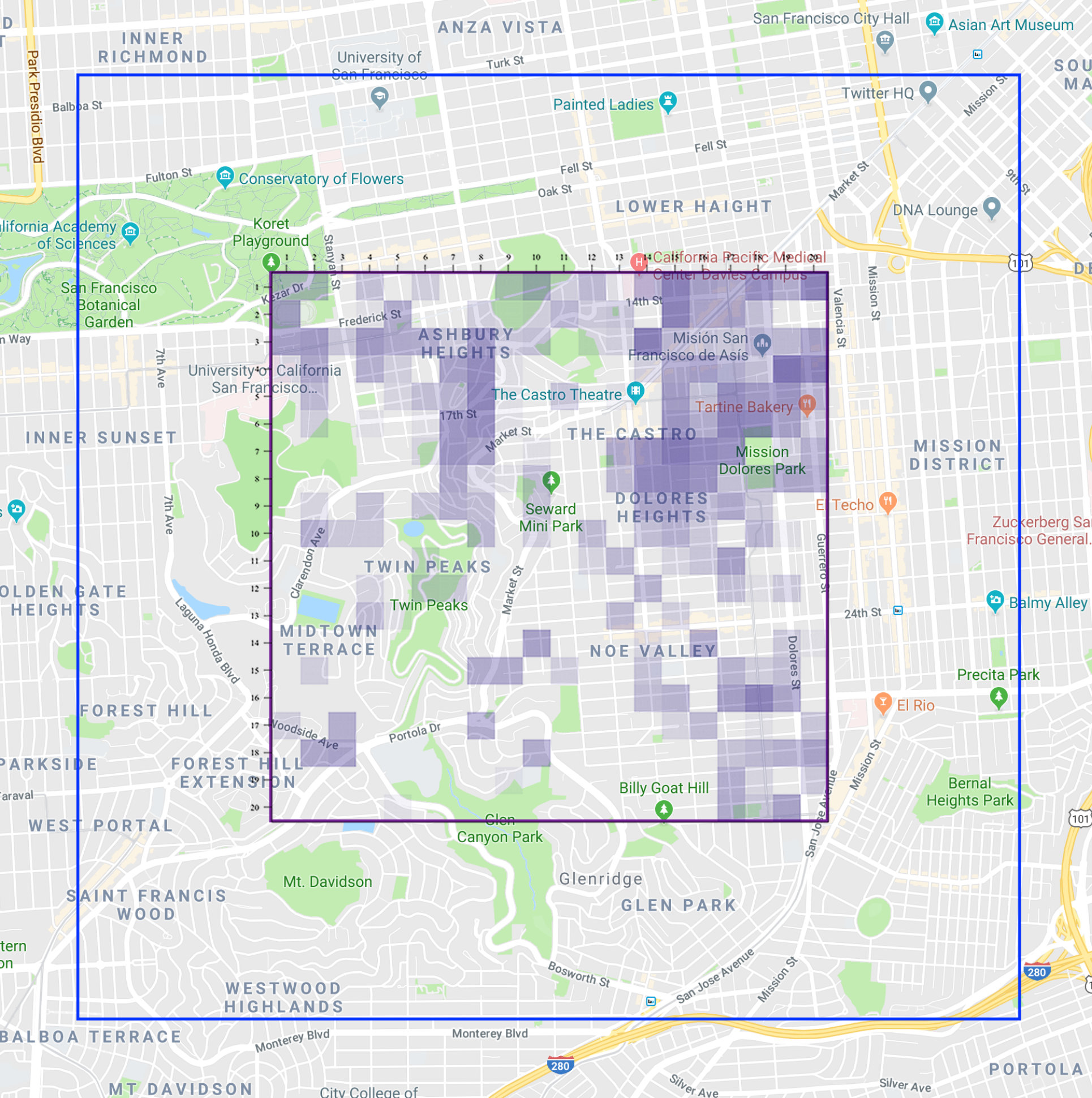 Figure 9
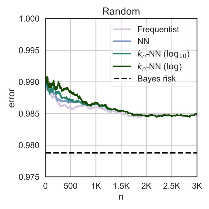 Figure 10
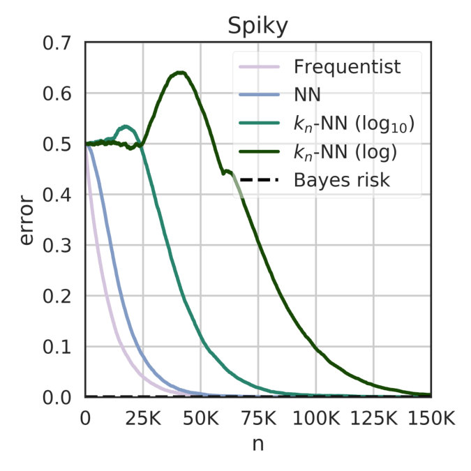 Figure 11
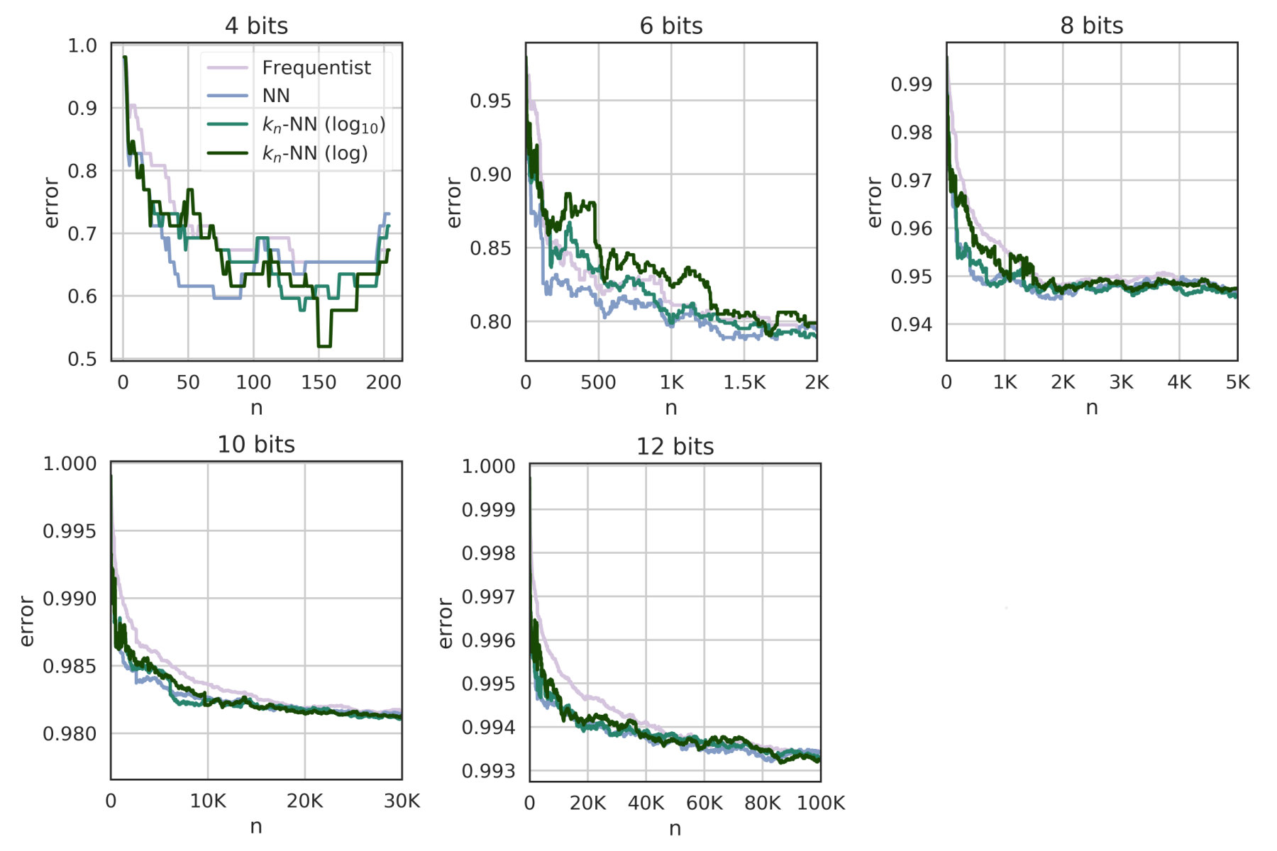 Figure 12
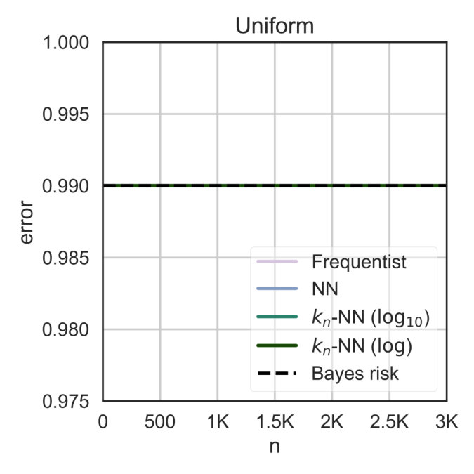 Figure 13
| System | Dataset | frequentist | NN | -NN |
|---|---|---|---|---|
| Random | 100 secrets, 100 obs. | 10 070 | 10 070 | 10 070 |
| Geometric () | 100 secrets, 10K obs. | 35 016 | 333 | 458 |
| Geometric () | 100 secrets, 10K obs. | 152 904 | 152 698 | 68 058 |
| Geometric () | 10K secrets, 1K obs. | 95 500 | 94 204 | 107 707 |
| Multimodal Geometric () | 100 secrets, 10K obs. | 44 715 | 568 | 754 |
| Spiky (contrived example) | 2 secrets, 10K obs. | 22 908 | 29 863 | 62 325 |
| Planar Geometric | Gowalla checkins in San Francisco area | X | X | 19 948 |
| Laplacian | " | N/A | X | 19 961 |
| Blahut-Arimoto | " | 1 285 | 1 170 | 1 343 |
| Symbol | Description |
|---|---|
| A secret | |
| An object/black-box output | |
| An example | |
| A system, given a set of priors and channel matrix | |
| Distribution induced by a system on | |
| A classifier | |
| Loss function w.r.t. which we evaluate a classifier | |
| The expected misclassification error of a classifier | |
| Bayes risk |
| Method | Guarantee | Space |
|---|---|---|
| frequentist | finite | |
| NN | finite | |
| -NN | infinite, separable | |
| NN Bound+ | infinite, separable |
| Name | Privacy parameter | |||
|---|---|---|---|---|
| Geometric | 1.0 | 100 | 10K | |
| Geometric | 0.1 | 100 | 10K | 0.007 |
| Geometric | 0.01 | 100 | 10K | 0.600 |
| Geometric | 0.2 | 100 | 1K | 0.364 |
| Geometric | 0.02 | 100 | 10K | 0.364 |
| Geometric | 0.002 | 100 | 100K | 0.364 |
| Geometric | 2 | 100K | 100K | 0.238 |
| Geometric | 2 | 100K | 10K | 0.924 |
| Multimodal | 1.0 | 100 | 10K | 0.450 |
| Multimodal | 0.1 | 100 | 10K | 0.456 |
| Multimodal | 0.01 | 100 | 10K | 0.797 |
| Spiky | N/A | 2 | 10K | 0 |
| Random | N/A | 100 | 100 | 0.979 |
| -NN | |||||
|---|---|---|---|---|---|
| System | Freq. | NN | |||
| Geometric = 1.0 | 0.1 | 1 994 | 267 | 396 | 679 |
| 0.05 | 4 216 | 325 | 458 | 781 | |
| 0.01 | 19 828 | 425 | 633 | 899 | |
| 0.005 | 38 621 | 439 | 698 | 904 | |
| Geometric = 0.1 | 0.1 | 18 110 | 269 | 396 | 673 |
| 0.05 | 35 016 | 333 | 458 | 768 | |
| 0.01 | 127 206 | 439 | 633 | 899 | |
| 0.005 | 211 742 | 4 844 | 698 | 904 | |
| Geometric = 0.01 | 0.1 | 105 453 | 103 357 | 99 852 | 34 243 |
| 0.05 | 205 824 | 205 266 | 205 263 | 199 604 | |
| -NN | |||||
|---|---|---|---|---|---|
| System | Freq. | NN | |||
| Multimodal = 1.0 | 0.1 | 3 008 | 369 | 478 | 897 |
| 0.05 | 5 938 | 495 | 754 | 1 267 | |
| 0.01 | 26 634 | 765 | 1 166 | 1 487 | |
| 0.005 | 52 081 | 765 | 1 166 | 1 487 | |
| Multimodal = 0.1 | 0.1 | 24 453 | 398 | 554 | 821 |
| 0.05 | 44 715 | 568 | 754 | 1 175 | |
| 0.01 | 149 244 | 4 842 | 1 166 | 1 487 | |
| 0.005 | 226 947 | 79 712 | 1 166 | 1 487 | |
| Multimodal = 0.01 | 0.1 | 27 489 | 753 | 900 | 381 |
| 0.05 | 103 374 | 101 664 | 92 181 | 31 452 | |
| Mechanism | Utility | ||
|---|---|---|---|
| Blahut-Arimoto | 2 | 0.760 | 334.611 |
| 4 | 0.571 | 160.839 | |
| 8 | 0.428 | 96.2724 | |
| Geometric | 2 | 0.657 | 288.372 |
| 4 | 0.456 | 144.233 | |
| 8 | 0.308 | 96.0195 | |
| Laplacian | 2 | 0.657 | 288.66 |
| 4 | 0.456 | 144.232 | |
| 8 | 0.308 | 96.212 |
| Operands’ size | ||
|---|---|---|
| 4 bits | 34 | |
| 6 bits | 123 | |
| 8 bits | 233 | |
| 10 bits | 371 | |
| 12 bits | 541 |
Peer Reviews
No public reviews on file for this paper yet. If you reviewed it on a platform where reviews are public (OpenReview, ICLR, NeurIPS, ICML), you can paste yours below so the community can read it here.
Code & Models
Videos
No videos yet. Explain this paper in a talk, walkthrough, or lecture? Add one.
F-BLEAU: Fast Black-box Leakage Estimation
Giovanni Cherubin
EPFL
Konstantinos Chatzikokolakis
University of Athens
Catuscia Palamidessi
INRIA, École Polytechnique
Abstract
We consider the problem of measuring how much a system reveals about its secret inputs. We work in the black-box setting: we assume no prior knowledge of the system’s internals, and we run the system for choices of secrets and measure its leakage from the respective outputs. Our goal is to estimate the Bayes risk, from which one can derive some of the most popular leakage measures (e.g., min-entropy leakage).
The state-of-the-art method for estimating these leakage measures is the frequentist paradigm, which approximates the system’s internals by looking at the frequencies of its inputs and outputs. Unfortunately, this does not scale for systems with large output spaces, where it would require too many input-output examples. Consequently, it also cannot be applied to systems with continuous outputs (e.g., time side channels, network traffic).
In this paper, we exploit an analogy between Machine Learning (ML) and black-box leakage estimation to show that the Bayes risk of a system can be estimated by using a class of ML methods: the universally consistent learning rules; these rules can exploit patterns in the input-output examples to improve the estimates’ convergence, while retaining formal optimality guarantees. We focus on a set of them, the nearest neighbor rules; we show that they significantly reduce the number of black-box queries required for a precise estimation whenever nearby outputs tend to be produced by the same secret; furthermore, some of them can tackle systems with continuous outputs. We illustrate the applicability of these techniques on both synthetic and real-world data, and we compare them with the state-of-the-art tool, leakiEst, which is based on the frequentist approach.
I Introduction
Measuring the information leakage of a system is one of the founding pillars of security. From side-channels to biases in random number generators, quantifying how much information a system leaks about its secret inputs is crucial for preventing adversaries from exploiting it; this has been the focus of intensive research efforts in the areas of privacy and of quantitative information flow (QIF). Most approaches in the literature are based on the white-box approach, which consists in calculating analytically the channel matrix of the system, constituted by the conditional probabilities of the outputs given the secrets, and then computing the desired leakage measures (for instance, mutual information [1], min-entropy leakage [2], or -leakage [3]). However, while one typically has white-box access to the system they want to secure, determining a system’s leakage analytically is often impractical, due to the size or complexity of its internals, or to the presence of unknown factors. These obstacles led to investigate methods for measuring a system’s leakage in a black-box manner.
Until a decade ago, the most popular measure of leakage was Shannon mutual information (MI). However, in his seminal paper [2] Smith showed that MI is not appropriate to represent a realistic attacker, and proposed a notion of leakage based on Rényi min-entropy (ME) instead. Consequently, in this paper we consider the general problem of estimating the Bayes risk of a system, which is the smallest error achievable by an adversary at predicting its secret inputs given the outputs. From the Bayes risk one can derive several leakage measures, including ME and the additive and multiplicative leakage [4]. These measures are considered by the QIF community among the most fundamental notions of leakage.
To the best of our knowledge, the only existing approach for the black-box estimation of the Bayes risk comes from a classical statistical technique, which refer to as the frequentist paradigm. The idea is to run the system repeatedly on chosen secret inputs, and then count the relative frequencies of the secrets and respective outputs so to estimate their joint probability distribution; from this distribution, it is then possible to compute estimates of the desired leakage measure. LeakWatch [5] and leakiEst [6], two well-known tools for black-box leakage estimation, are applications of this principle.
Unfortunately, the frequentist approach does not always scale for real-world problems: as the number of possible input and output values of the channel matrix increases, the number of examples required for this method to converge becomes too large to gather. For example, LeakWatch requires a number of examples that is much larger than the product of the size of input and output space. For the same reason, this method cannot be used for systems with continuous outputs; indeed, it cannot even be formally constructed in such a case.
Our contribution
In this paper, we show that machine learning (ML) methods can provide the necessary scalability to black-box measurements, and yet maintain formal guarantees on their estimates. By observing a fundamental equivalence between ML and black-box leakage estimation, we show that any ML rule from a certain class (the universally consistent rules) can be used to estimate with arbitrary precision the leakage of a system. In particular, we study rules based on the nearest neighbor principle – namely, Nearest Neighbor (NN) and -NN, which exploit a metric on the output space to achieve a considerably faster convergence than frequentist approaches. In Table I we summarize the number of examples necessary for the estimators to converge, for the various systems considered in the paper. We focus on nearest neighbor methods, among the existing universally consistent rules, because: i) they are simple to reason about, and ii) we can identify the class of systems for which they will excel, which happens whenever the distribution is somehow regular with respect to a metric on the output (e.g., time side channels, traffic analysis, and most mechanisms used for privacy). Moreover, some of these methods can tackle directly systems with continuous output.
We evaluate these estimators on synthetic data, where we know the true distributions and we can determine exactly when the estimates converge. Furthermore, we use them for measuring the leakage in a real dataset of users’ locations, defended with three state-of-the-art mechanisms: two geo-indistinguishability mechanisms (planar geometric and planar Laplacian)[7], and the method by Oya et al. [8], which we refer to as the Blahut-Arimoto mechanism. Crucially, the planar Laplacian is real-valued, which -NN methods can tackle out-of-the box, but the frequentist method cannot. Results in both synthetic and real-world data show our methods give a strong advantage whenever there is a notion of metric in the output that can be exploited. Finally, we compare our methods with leakiEst on the problem of estimating the leakage of European passports [9, 6], and on the location privacy data.
As a further evidence of their practicality, we use them in Appendix G to measure the leakage of a time side channel in a hardware implementation of finite field exponentiation.
No Free Lunch
A central takeaway of our work is that, while all the estimators we study (including the frequentist approach) are asymptotically optimal in the number of examples, none of them can guarantee on its finite sample performance; indeed, no estimator can. This is a consequence of the No Free Lunch theorem in ML [10], which informally states that all learning rules are equivalent among the possible distributions of data. This rules out the existence of an optimal estimator.
In practice, this means that we should always evaluate several estimators, and select the one that converged faster. Fortunately, our main finding (i.e., any universally consistent ML rule is a leakage estimator) adds a whole new class of estimators, which one can use in practical applications.
We therefore propose a tool, F-BLEAU (Fast Black-box Leakage Estimation AUtomated), which computes nearest neighbor and frequentist estimates, and selects the one converging faster. We release it as Open Source software111https://github.com/gchers/fbleau., and we hope in the future to extend it to support several more estimators based on UC ML rules.
Nearest Neighbor rules
Nearest neighbor rules excel whenever there is a notion of metric on the output space, and the output distributions is “regular” (in the sense that it does not change too abruptly between two neighboring points). We expect this to be the case for several real-world systems, such as: side channels whose output is time, an electromagnetic signal, or power consumption; for traffic analysis on network packets; and for geographic location data. Moreover, most mechanisms used in privacy and QIF use smooth noise distributions. Suitable applications may also come from recent attacks to ML models, such as model inversion [11] and membership inference [12].
Furthermore, we observe that even when there is no metric, or when the output distribution is irregular, (e.g., a system whose internal distribution has been randomly sampled), these rules are equivalent to the frequentist approach. Indeed, the only case we observe when they are misled is when the system is crafted so that the metric contributes against classification (e.g., see “Spiky” example in Table I).
II Related Work
Chatzikokolakis et al. [13] introduced methods for measuring the leakage of a deterministic program in a black-box manner; these methods worked by collecting a large number of inputs and respective outputs, and by estimating the underlying probability distribution accordingly; this is what we refer to as the frequentist paradigm. A fundamental development of their work by Boreale and Paolini [14] showed that, in the absence of significant a priori information about the output distribution, no estimator does better than the exhaustive enumeration of the input domain. In line with this work, section IV will show that, as a consequence of the No Free Lunch theorem in ML, no leakage estimator can claim to converge faster than any other estimator for all distributions.
The best known tools for black-box estimation of leakage measures based on the Bayes risk (e.g., min-entropy) are leakiEst [15, 6] and LeakWatch [5, 16], both based on the frequentist paradigm. The former also allows a zero-leakage test for systems with continuous outputs. In LABEL:sec:comparison we provide a comparison of leakiEst with our proposal.
Cherubin [17] used the guarantees of nearest neighbor learning rules for estimating the information leakage (in terms of the Bayes risk) of defenses against website fingerprinting attacks in a black-box manner.
Shannon mutual information (MI) is the main alternative to the Bayes risk-based notions of leakage in the QIF literature. Although there is a relation between MI and Bayes risk [18], the corresponding models of attackers are very different: the first corresponds to an attacker who can try infinitely many times to guess the secret, while the second has only one try at his disposal [2]. Consequently, MI and Bayes-risk measures, such as ME, can give very different results: Smith [2] shows two programs that have almost the same MI, but one has an ME several orders of magnitude larger than the other one; conversely, there are examples of two programs such that ME is [math] for both, while the MI is [math] in one case and strictly positive (several bits) in the other one.
In the black-box literature, MI is usually computed by using Kernel Density Estimation, which although only guarantees asymptotic optimality under smoothness assumptions on the distributions. On the other hand, the ML literature offered developments in this area: Belghazi et al. [19] proposed an MI lower bound estimator based on deep neural networks, and proved its consistency (i.e., it converges to the true MI value asymptotically). Similarly, other works constructed MI variational lower bounds [20, 21].
III Preliminaries
We define a system, and show that its leakage can be expressed in terms of the Bayes risk. We then introduce ML notions, which we will later use to estimate the Bayes risk.
III-A Notation
We consider a system , that associates a secret input to an observation (or object) in a possibly randomized way. The system is defined by a set of prior probabilities , , and a channel matrix of size , for which for and . We call the example space. We assume the system does not change over time; for us, is finite, and is finite unless otherwise stated.
III-B Leakage Measures
The state-of-the-art in QIF is represented by the leakage measures based on -vulnerability, a family whose most representative member is min-vulnerability [2], the complement of the Bayes risk. This paper is concerned with finding tight estimates of the Bayes risk, which can then be used to estimate the appropriate leakage measure.
Bayes risk
The Bayes risk, , is the error of the optimal (idealized) classifier for the task of predicting a secret given an observation output by a system. It is defined with respect to a loss function , where is the risk of an adversary predicting for an observation , when its actual secret is . We focus on the 0-1 loss function, , taking value if , [math] otherwise. The Bayes risk of a system is defined as:
[TABLE]
Random guessing
A baseline for evaluating a system is the error committed by an idealized adversary who knows priors but has no access to the channel, and who’s best strategy is to always output the secret with the highest prior. We call the error of this adversary random guessing error:
[TABLE]
III-C Black-box estimation of
This paper is concerned with estimating the Bayes risk given examples sampled from the joint distribution on generated by . By running the system times on secrets , chosen according to , we generate a sequence of corresponding outputs , thus forming a training set222In line with the ML literature, we call the training or test “set” what is technically a multiset; also, we loosely use the set notation “” for both sets and multisets when the nature of the object is clear from the context. of examples . From these data, we aim to make an estimate close to the real Bayes risk.
III-D Learning Rules
We introduce ML rules (or, simply, learning rules), which are algorithms for selecting a classifier given a set of training examples. In this paper, we will use the error of some ML rules as an estimator of the Bayes risk.
Let be a set of classifiers. A learning rule is a possibly randomized algorithm that, given a training set , returns a classifier , with the goal of minimizing the expected loss for a new example sampled from [22]. In the case of the 0-1 loss function, the expected loss coincides with the expected probability of error (expected error for short), and if is generated by a system , then the expected error of a classifier is:
[TABLE]
where is the secret predicted for object . If is infinite (and is continuous) the summation is replaced by an integral.
III-E Frequentist estimate of
The frequentist paradigm [13] for measuring the leakage of a channel consists in estimating the probabilities by counting their frequency in the training data :
[TABLE]
We can obtain the frequentist error from Equation 3:
[TABLE]
where is the frequentist classifier, namely:
[TABLE]
where is estimated from the examples: .
Consider a finite example space . Provided with enough examples, the frequentist approach always converges: clearly, as , because events’ frequencies converge to their probabilities by the Law of Large Numbers.
However, there is a fundamental issue with this approach. Given a training set , the frequentist classifier can tell something meaningful (i.e., better than random guessing) for an object , only as long as appeared in the training set; but, for very large systems (e.g., those with a large object space), the probability of observing an example for each object becomes small, and the frequentist classifier approaches random guessing. We study this matter further in LABEL:subsec:random-system and Appendix E.
IV No Free Lunch In Learning
The frequentist approach performs well only for objects it has seen in the training data; in the next section, we will introduce estimators that aim to provide good predictions even for unseen objects. However, we shall first answer an important question: is there an estimator that is “optimal” for all systems?
A negative answer to this question is given by the so-called “No Free Lunch” (NFL) theorem by Wolpert [10]. The theorem is formulated for the expected loss of a learning rule on unseen objects (i.e., that were not in the training data), which is referred to as the off-training-set (OTS) loss.
Theorem 1** (No Free Lunch).**
Let and be two learning rules, a cost function, and a distribution on . We indicate by the OTS loss of given and , where the expectation is computed over all the possible training sets of size sampled from . Then, if we take the uniform average among all possible distributions , we have
[TABLE]
Intuitively, the NFL theorem says that, if all distributions (and, therefore, all channel matrices) are equally likely, then all learning algorithms are equivalent. Remarkably, this holds for any strategy, even if one of the rules is random guessing.
An important implication of this for our purposes is that for every two learning rules and there will always exist some system for which rule converges faster than , and vice versa there will be a system for which outperforms .
From the practical perspective of black-box security, this demonstrates that we should always test several estimators and select the one that converges faster. Fortunately, the connection between ML and black-box security we highlight in this paper results in the discovery of a whole class of new estimators.
V Machine Learning Estimates of the Bayes Risk
In this section, we define the notion of a universally consistent learning rule, and show that the error of a classifier selected according to such a rule can be used for estimating the Bayes risk. Then, we introduce various universally consistent rules based on the nearest neighbor principle.
Throughout the section, we use interchangeably a system and its corresponding joint distribution on . Note that there is a one-to-one correspondence between them.
V-A Universally Consistent Rules
Consider a distribution and a learning rule selecting a classifier according to training examples sampled from . Intuitively, as the available training data increases, we would like the expected error of for a new example sampled from to be minimized (i.e., to get close the Bayes risk). The following definition captures this intuition.
Definition 1** (Consistent Learning Rule).**
Let be a distribution on and let be a learning rule. Let be a classifier selected by using training examples sampled from . Let be the system corresponding to , and let be the expected error of , as defined by (3). We say that is consistent if as .
The next definition strengthens this property, by asking the rule to be consistent for all distributions:
Definition 2** (Universally Consistent (UC) Learning Rule).**
A learning rule is universally consistent if it is consistent for any distribution on .
By this definition, the expected error of a classifier selected according to a universally consistent rule is also an estimator of the Bayes risk, since it converges to as .
In the rest of this section we introduce Bayes risk estimates based on universally consistent nearest neighbor rules; they are summarized in Table III together with their guarantees.
V-B NN estimate
The Nearest Neighbor (NN) is one of the simplest ML classifiers: given a training set and a new object , it predicts the secret of its closest training observation (nearest neighbor). It is defined both for finite and infinite object spaces, although it is UC only in the first case.
We introduce a formulation of NN, which can be seen as an extension of the frequentist approach, that takes into account ties (i.e., neighbors that are equally close to the new object ), and which guarantees consistency when is finite.
Consider a training set , an object , and a distance metric . The NN classifier predicts a secret for by taking a majority vote over the set of secrets whose objects have the smallest distance to . Formally, let and define:
[TABLE]
where
[TABLE]
We show that NN is universally consistent for finite .
Theorem 2** (Universal consistency of NN).**
Consider a distribution on , where and are finite. Let be the expected error of the NN classifier for a new observation . As the number of training examples :
[TABLE]
Sketch proof.
For an observation that appears in the training set, the NN classifier is equivalent to the frequentist approach. For a finite space , as , the probability that the training set contains all approaches . Thus, the NN rule is asymptotically (in ) equivalent to the frequentist approach, which means its error also converges to . ∎
V-C -NN estimate
Whilst NN guarantees universal consistency in finite example spaces, this does not hold for infinite . In this case, we can achieve universal consistency with the k-NN classifier, an extension of NN, for appropriate choices of the parameter .
The k-NN classifier takes a majority vote among the secrets of its neighbors. Breaking ties in the k-NN definition requires more care than with NN. In the literature, this is generally done via strategies that add randomness or arbitrariness to the choice (e.g., if two neighbors have the same distance, select the one with the smallest index in the training data) [23]. We use a novel tie-breaking strategy, which takes into account ties, but gives more importance to the closest neighbors. In early experiments, we observed this strategy had a faster convergence than standard approaches.
Consider a training set , an object to predict , and some metric . Let denote the -th closest object to , and its respective secret. If ties do not occur after the -th neighbor (i.e., if ), then k-NN outputs the most frequent among the secrets of the first neighbors:
[TABLE]
where
[TABLE]
If ties exist after the -th neighbor, that is, for :
[TABLE]
we proceed as follows. Let be the most frequent secret in ; k-NN predicts the most frequent secret in the following multiset, truncated at the tail to have size :
[TABLE]
We now define -NN, a universally consistent learning rule that selects a k-NN classifier for a training set of examples by choosing as a function of .
Definition 3** (-NN rule).**
Given a training set of examples, the -NN rule selects a k-NN classifier, where is chosen such that and as .
Stone proved that -NN is universally consistent [24]:
Theorem 3** (Universal consistency of the -NN rule).**
Consider a probability distribution on the example space , where has a density. Select a distance metric such that is separable333A separable space is a space containing a countable dense subset; e.g., finite spaces and the space of -dimensional vectors with Euclidean metric.. Then the expected error of the -NN rule converges to as .
This holds for any distance metric. In our experiments, we will use the Euclidean distance, and we will evaluate -NN rules for (natural logarithm) and .
The ML literature is rich of UC rules and other useful tools for black-box security; we list some of them in Appendix A.
VI Evaluation on Synthetic Data
In this section we evaluate our estimates on several synthetic systems for which the channel matrix is known. For each system, we sample examples from its distribution, and then compute the estimate on the whole object space as in Equation 3; this is possible because is finite. Since for synthetic data we know the real Bayes risk, we can measure how many examples are required for the convergence of each estimate. We do this as follows: let be an estimate of , trained on a dataset of examples. We say the estimate -converged to after examples if its relative change from is smaller than :
[TABLE]
While relative change has the advantage of taking into account the magnitude of the compared values, it is not defined when the denominator is [math]; therefore, when (Table IV), we verify convergence with the absolute change:
[TABLE]
The systems used in our experiments are briefly discussed in this section, and summarized in Table IV; we detail them in Appendix B. A uniform prior is assumed in all cases.
VI-A Geometric systems
We first consider systems generated by adding geometric noise to the secret, one of the typical mechanisms used to implement differential privacy [25]. Their channel matrix has the following form:
[TABLE]
where is a privacy parameter, a normalization factor, and a function ; a detailed description of these systems is given in in Appendix B.
We consider the following three parameters:
- •
the privacy parameter ,
- •
the ratio , and
- •
the size of the secret space .
We vary each of these parameters one at a time, to isolate their effect on the convergence rate.
VI-A1 Variation of the privacy parameter
We fix , K, and we consider three cases , and . The results for the estimation of the Bayes risk and the convergence rate are illustrated in Figure 1 and subsubsection VI-A1 respectively. In the table, results are reported for convergence level ; an “X” means a particular estimate did not converge within 500K examples; a missing row for a certain means no estimate converged.
The results indicate that the nearest neighbor methods have a much faster convergence than the standard frequentist approach, particularly when dealing with large systems. The reason is that geometric systems have a regular behavior with respect to the Euclidean metric, which can be exploited by NN and -NN to make good predictions for unseen objects.
The reference list from the paper itself. Each links out to its DOI / PubMed record.
- 1[1] D. Clark, S. Hunt, and P. Malacaria, “Quantitative information flow, relations and polymorphic types,” J. of Logic and Computation , vol. 18, no. 2, pp. 181–199, 2005.
- 2[2] G. Smith, “On the foundations of quantitative information flow,” in Proceedings of the 12th International Conference on Foundations of Software Science and Computation Structures (FOSSACS 2009) , ser. LNCS, L. de Alfaro, Ed., vol. 5504. York, UK: Springer, 2009, pp. 288–302.
- 3[3] M. S. Alvim, K. Chatzikokolakis, C. Palamidessi, and G. Smith, “Measuring information leakage using generalized gain functions,” in Proceedings of the 25th IEEE Computer Security Foundations Symposium (CSF) , 2012, pp. 265–279. [Online]. Available: http://hal.inria.fr/hal-00734044/en
- 4[4] C. Braun, K. Chatzikokolakis, and C. Palamidessi, “Quantitative notions of leakage for one-try attacks,” in Proceedings of the 25th Conf. on Mathematical Foundations of Programming Semantics , ser. Electronic Notes in Theoretical Computer Science, vol. 249. Elsevier B.V., 2009, pp. 75–91. [Online]. Available: http://hal.archives-ouvertes.fr/inria-00424852/en/
- 5[5] T. Chothia, Y. Kawamoto, and C. Novakovic, “Leak Watch: Estimating information leakage from java programs,” in Proc. of ESORICS 2014 Part II , 2014, pp. 219–236.
- 6[6] ——, “A tool for estimating information leakage,” in International Conference on Computer Aided Verification (CAV) . Springer, 2013, pp. 690–695.
- 7[7] M. E. Andrés, N. E. Bordenabe, K. Chatzikokolakis, and C. Palamidessi, “Geo-indistinguishability: Differential privacy for location-based systems,” in Proceedings of the 2013 ACM SIGSAC conference on Computer & communications security . ACM, 2013, pp. 901–914.
- 8[8] S. Oya, C. Troncoso, and F. Pérez-González, “Back to the drawing board: Revisiting the design of optimal location privacy-preserving mechanisms,” in Proceedings of the 2017 ACM SIGSAC Conference on Computer and Communications Security , ser. CCS ’17. ACM, 2017, pp. 1959–1972. [Online]. Available: http://doi.acm.org/10.1145/3133956.3134004
