Ordinal Patterns in Clusters of Subsequent Extremes of Regularly Varying Time Series
Marco Oesting, Alexander Schnurr

TL;DR
This paper studies the structure of clusters of extreme events in time series, focusing on their size distribution and ordinal patterns, with methods applicable to real-world data like river discharge measurements.
Contribution
It introduces non-parametric estimators for cluster size and ordinal patterns, proves their asymptotic properties, and demonstrates their effectiveness through simulations and real data.
Findings
Limit distributions for cluster features are established.
Estimators perform well in simulations.
Application to river discharge data reveals meaningful patterns.
Abstract
In this paper, we investigate temporal clusters of extremes defined as subsequent exceedances of high thresholds in a stationary time series. Two meaningful features of these clusters are the probability distribution of the cluster size and the ordinal patterns within a cluster. Since these patterns take only the ordinal structure of consecutive data points into account the method is robust under monotone transformations and measurement errors. We verify the existence of the corresponding limit distributions in the framework of regularly varying time series, develop non-parametric estimators and show their asymptotic normality under appropriate mixing conditions. The performance of the estimators is demonstrated in a simulated example and a real data application to discharge data of the river Rhine.
Click any figure to enlarge with its caption.
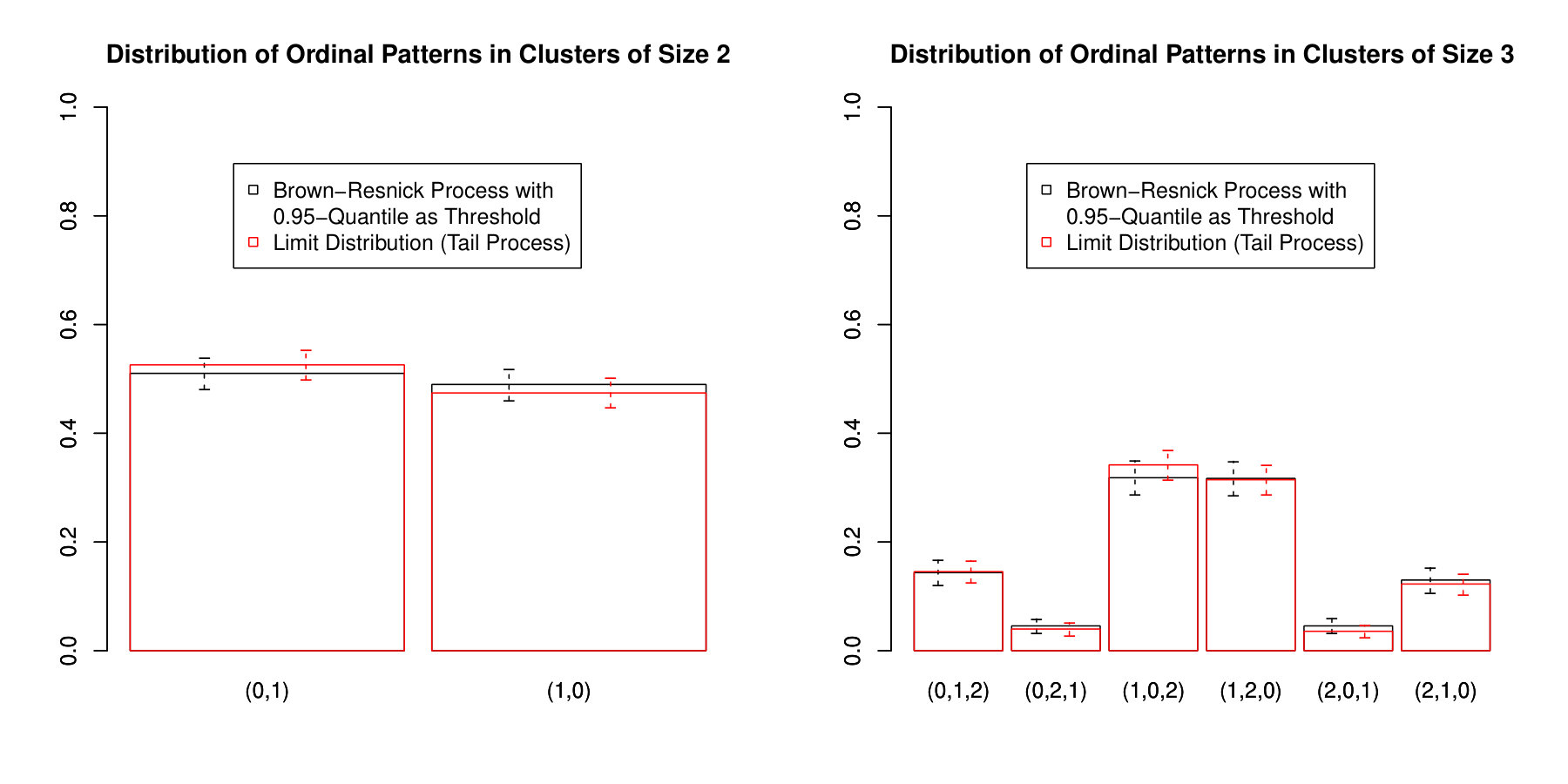 Figure 1
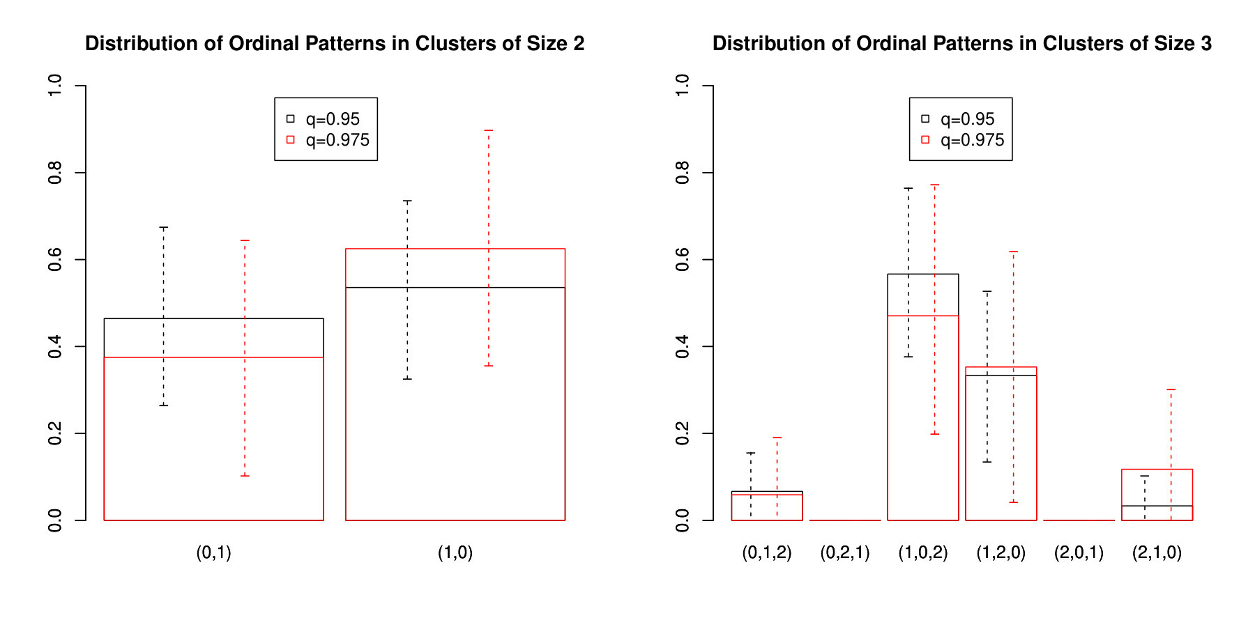 Figure 2
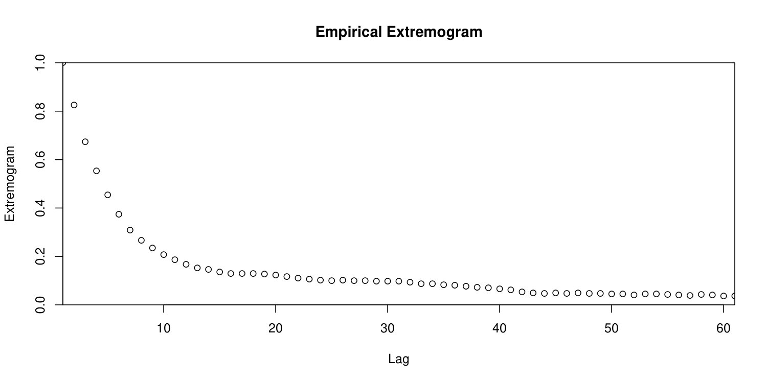 Figure 3
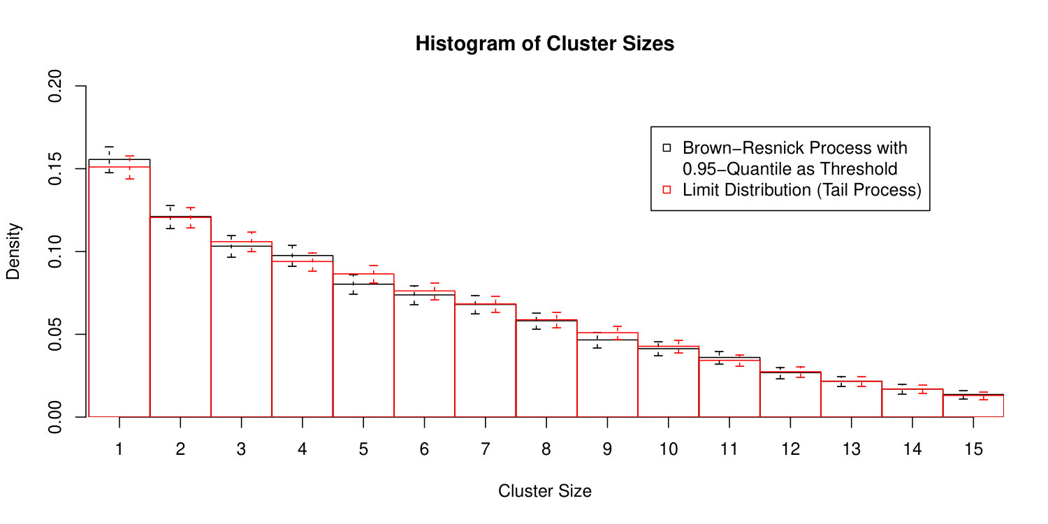 Figure 4
Peer Reviews
No public reviews on file for this paper yet. If you reviewed it on a platform where reviews are public (OpenReview, ICLR, NeurIPS, ICML), you can paste yours below so the community can read it here.
Videos
No videos yet. Explain this paper in a talk, walkthrough, or lecture? Add one.
Ordinal Patterns in Clusters of Subsequent Extremes of Regularly Varying Time Series
Marco Oesting and Alexander Schnurr University of Siegen, Department Mathematik, Walter-Flex-Str. 3, 57068 Siegen, Germany, Email: [email protected] of Siegen, Department Mathematik, Walter-Flex-Str. 3, 57068 Siegen, Germany, Email: [email protected]
Abstract
In this paper, we investigate temporal clusters of extremes defined as subsequent exceedances of high thresholds in a stationary time series. Two meaningful features of these clusters are the probability distribution of the cluster size and the ordinal patterns giving the relative positions of the data points within a cluster. Since these patterns take only the ordinal structure of consecutive data points into account, the method is robust under monotone transformations and measurement errors. We verify the existence of the corresponding limit distributions in the framework of regularly varying time series, develop non-parametric estimators and show their asymptotic normality under appropriate mixing conditions. The performance of the estimators is demonstrated in a simulated example and a real data application to discharge data of the river Rhine.
1 Introduction
In time series data sets, extremes often do not occur at scattered instants of time, but tend to form clusters. Assigning a cluster of extremes to a single extreme event, such as a flood in the context of a hydrological time series or a stock market crash in the context of a financial data, the distribution of these clusters is crucial for risk assessment.
In order to analyze the occurrence times of extremes defined as exceedances over some high threshold , some profound theory has been built up since the 1970s. Within this framework, data from a stationary time series are typically divided into different blocks. Then, repeated extremes are said to form a cluster if they occur within the same temporal block. Due to the convergence of the process of exceedances to a Poisson point process under appropriate conditions as , the distribution of these clusters converges weakly provided that the block size increases at the right speed. The limit distribution is nicely linked to the well-known concept of the extremal index of the time series which can be interpreted as the reciprocal of the mean limiting cluster size (cf. Leadbetter et al., 1983; Embrechts et al., 1997; Chavez-Demoulin and Davison, 2012, for an overview). Besides the extremal index, several other cluster characteristics are of interest and can be estimated, such as the distribution of the cluster size (Robert, 2009) or more general cluster functionals (Drees and Rootzén, 2010). Convergence of clusters in appropriate sequence spaces preserving the order of observations can be shown within the framework of regular variation (Basrak et al., 2018).
Even though positive theoretical results exist, estimation of characteristics of clusters as defined above is difficult for finite samples. Here, besides the threshold , also the block size or, equivalently, some cluster identification parameter giving the minimum distance between two separate clusters, needs to be chosen. Instead, in this paper, we will use a different definition of a cluster of extremes by restricting our attention to subsequent threshold exceedances, i.e. a realization of the -dimensional vector will be called a -exceedance cluster of size if and only if
[TABLE]
As any non-exceedance will separate two clusters, this definition is much stricter than the classical definition described above. An advantage of the definition of -exceedance clusters is that it depends on one parameter, namely the threshold , only. Such a cluster definition has already been employed in a series of papers by Markovich (2014, 2016, 2017) who analyzes the limit distribution of two cluster characteristics. First, she considers the number of inter-cluster times , i.e. the number of observations between two consecutive clusters, which is a random variable with the same distribution as
[TABLE]
Note that this number of inter-cluster time also plays an important role in the estimation of the extremal index (Ferro and Segers, 2003). Secondly, she studies the random variable with the same distribution as
[TABLE]
i.e. is the length of a -exceedance cluster starting at some fixed time. Since we have , the distribution of is typically expected to converge weakly to a degenerate distribution, i.e. . In Markovich (2014, 2016), under appropriate mixing conditions, the rate of convergence is determined as a function of the extremal index. More precisely, for all , there exist a threshold a number such that, for all and ,
[TABLE]
i.e. for a sufficiently large threshold , the tail of the distribution of becomes proportional to a geometric distribution with parameter . Furthermore, Markovich (2014, 2016) provides results for the duration of clusters if the time between subsequent observations is random.
In our paper, we will focus on the case of an equally spaced time series, i.e. the case when the terms of the duration and the size of cluster coincide. Here, instead of considering the probability that there is a cluster of a specific size at a certain time, we analyze the size of a randomly chosen -exceedance cluster or, equivalently, we examine the size of a cluster conditional on being a cluster of positive length. Thus, we first address the question:
How long does an extreme event in a time series last provided that it occurs?
Secondly, we analyze so-called ordinal patterns which we find in the above mentioned clusters of extremes. Ordinal patterns keep the ordinal information of the data only and, thus, describe their ‘up-and-down behaviour’. Here, the relative position of the data points is encoded by a permutation on such that
[TABLE]
Note that this permutation is unique if the data points are pairwise distinct. The following precise definition also accounts for the ties by keeping the order of the indices in this case.
Definition 1.1**.**
For , let be the set of permutations of . The -ordinal pattern is defined as the mapping that maps a vector to the unique permutation satisfying
[TABLE]
and if for .
Ordinal patterns have been introduced in order to analyze noisy data sets which appear in medicine, neuroscience and finance (cf. Bandt and Pompe, 2002; Keller et al., 2007; Sinn et al., 2013). They have already been used successfully in the estimation of the Hurst parameter (Sinn and Keller, 2011). Further applications include tests for structural breaks (Sinn et al., 2012) and the analysis of the Kolmogorov-Sinai entropy of dynamical systems (Keller et al., 2015).
Ordinal patterns can be used nicely to capture stylized facts as trends or inversions of the direction which might be used to characterize and classify certain events. To our knowledge the present paper is the first approach to analyze the ordinal behavior which can be observed in clusters of extremes of time series. The advantages of the proposed method include that the whole analysis is stable under monotone transformations of the state space. This will be useful in our analysis. Furthermore, the ordinal structure is not destroyed by small perturbations of the data or by measurement errors. There are fast algorithms to analyze the relative frequencies of ordinal patterns in given data sets (cf. Keller et al., 2007, Section 1.4).
In the future, ordinal patterns in clusters of extremes might be used to detect structural breaks in the extremes of the given time series (cf. Unakafov and Keller, 2018). Dealing with ‘correlated’ time series, one could analyze the dependence between extreme events in a non-linear fashion as it has been developed in Schnurr (2014) and Schnurr and Dehling (2017). This might be advantageous in particular if the time series are on totally different scales. Finally, as we will point out in Section 6, ordinal patterns at the beginning of a cluster of extremes might be used in order to forecast the length of this cluster in an on-line analysis of data.
Our analysis is embedded in a different theoretical framework than the works of Markovich (2014, 2016, 2017), namely, we will assume that the stationary time series of interest, , is regularly varying. Note that this is a common assumption in extreme value theory allowing for convenient extrapolation to the tails of the distribution. More background on the theory of regularly varying time series will be provided in Section 2. In Section 3, we show that both the distribution of the size of -exceedance clusters, as defined in (1), and the distribution of the ordinal pattern within a cluster converge to (typically non-degenerate) limit distributions in case of a regularly varying time series. Based on a sliding window approach, non-parametric empirical estimators for the limit distributions are introduced in Section 4. Under conditions, similar to those considered in Davis and Mikosch (2009) for the estimation of the extremogram, consistency (Proposition 4.1) and asymptotic normality (Corollary 4.6) of the estimators are established. In Section 5, we consider the example of max-stable time series and provide sufficient conditions in terms of extremal coefficients for Corollary 4.6 to hold. The conditions are verified for a Brown–Resnick time series which is then simulated to demonstrate the finite-sample behaviour of the estimators. Finally, we apply the estimator to daily discharge data of the river Rhine at Cologne in Section 6. The proofs of our results can be found in the appendix.
2 Background: Regular Varying Time Series
Throughout this paper, we will assume that is a stationary time series whose marginal distribution , defined by , is in the max-domain of attraction of an extreme value distribution, i.e., there exist constants , , such that
[TABLE]
for some non-degenerate distribution . Without loss of generality, we may assume that is an -Fréchet distribution for some ,
[TABLE]
and that has a finite lower endpoint, . Both properties can be achieved by applying strictly monotone marginal transformations to provided that is continuous. As these transformations are the same for each – remind that is stationary – they do not have any effect on ordinal structure of the data. In particular, ordinal patterns in extremes are invariant under these transformations.
A convenient framework for our further analysis will be provided by regular variation. Among several equivalent definitions of multivariate regular variation (cf. Resnick, 2007, 2008, for instance), we will make use of the following convenient one (cf. Basrak et al., 2002, for instance): We say that the -variate random vector , , is multivariate regularly varying with index if, for some norm on , there exists a probability measure on the sphere such that
[TABLE]
as , where denotes weak convergence. The limit measure is called spectral measure.
By Corollary 5.18 in Resnick (2008), multivariate regular variation of with spectral measure is equivalent to the fact that the distribution function of is in the max-domain of attraction of a multivariate extreme value distribution, i.e.
[TABLE]
The limit distribution necessarily has marginal distributions and is of the form
[TABLE]
for some Radon measure on , the so-called exponent measure of . The exponent measure and the spectral measure are related via
[TABLE]
The time series is called regularly varying if all the finite-dimensional margins , , , are multivariate regularly varying. By Basrak and Segers (2009), regular variation of is equivalent to the existence of a process with for such that, for every ,
[TABLE]
The process is called tail process of , see Basrak and Segers (2009) and Planinić and Soulier (2018) for more details and further properties.
In the following, we will always assume that the time series is regularly varying with tail process . Furthermore, the probability measure induced by the random vector will be called for any index set .
3 Distribution of Clusters of Extremes and Ordinal Patterns
In this section, we will analyze the limiting behaviour of the size and ordinal pattern of -exceedance clusters in the time series with -exceedances being defined as in (1). Intuitively, the following expression gives a plausible definition of the distribution of the size of a randomly selected -exceedance cluster:
[TABLE]
If is ergodic, we can apply the pointwise Birkhoff-Khinchin theorem and obtain that the above limit almost surely exists and equals
[TABLE]
Dividing both the enumerator and the denominator of (3) by , we can see from relation (2) that the distribution of eventually becomes independent from the threshold as provided that
[TABLE]
for every :
[TABLE]
Example 3.1**.**
We consider two examples to compare the limiting distribution of as , i.e. the distribution of the cluster size according to our definition, with the limiting cluster size distribution in the classical setting which has been studied extensively in the literature, cf. Robert (2009) and references therein. While both distributions coincide in the first examples, they significantly differ in the second one.
We consider a first order max-autoregressive model (cf. Davis and Resnick, 1989)
[TABLE]
where and is a unit Fréchet noise process. Equation (5) possesses a stationary solution with unit Fréchet margins that is regularly varying. For , the tail process is given by
[TABLE]
where is a standard Pareto random variable. Furthermore, we have
[TABLE]
Thus, for , we obtain
[TABLE]
i.e. the limiting distribution is a geometric distribution with parameter . Alternatively, this distribution could also be derived from Proposition 1 in Markovich (2017) plugging the formulae for into the expression and using that the extremal index is given by . However, obtaining a closed-form expression seems to be much simpler using the tail process.
Note that the limiting geometric distribution in (6) coincides with the limiting distribution for the size of clusters defined in the classical sense, cf. Perfekt (1994). This is due to the fact that, in the limit, exceedances over high thresholds always occur subsequently. 2. 2.
As second example, we consider a stationary moving maximum process (cf. Deheuvels, 1983, for instance) defined by
[TABLE]
with being a unit Fréchet noise process. By definition, we have that for all . Consequently,
[TABLE]
i.e. the distribution of converges weakly to a Dirac measure in .
In contrast, the limiting cluster size distribution according to the classical definition is obviously a Dirac measure in , that is, exceedances over high thresholds always occur in pairs. As the exceedances are separated by a non-exceedance, each pair is considered as two single clusters in our definition, while they belong to the same cluster according to the classical definition.
Similarly to their size, we can investigate ordinal patterns in -exceedance clusters. Here, for fixed , we are interested in the distribution of the -ordinal pattern of a (randomly selected) -exceedance cluster of size :
[TABLE]
for each , i.e. defines a probability distribution on . Again, this distribution converges as :
[TABLE]
4 Asymptotic Results for Empirical Estimators
According to Equation (4) and Equation (7), both the limit distribution of clusters and the limit distribution of ordinal patterns within a cluster are given by a ratio of the type
[TABLE]
for appropriate dimension and sets and with , i.e. a ratio of measures of two sets that are bounded from below by in their second component.
More precisely, in case of the cluster size distribution in (4), we have , , and , while, in case of the distribution of the -ordinal pattern in (7), we have , and .
In the following, we will consider the general class of ratios of the above type, including both the limits in (4) and (7) as special cases, and discuss their estimation from observations . It is worth noting that, making use of relation , we may replace and by the maximum of the two, i.e. without loss of generality, we may assume that .
Analogously to the calculations in Section 3, one can show that
[TABLE]
provided that . This limit relation gives reason to set a high threshold and use a ratio estimator of the type
[TABLE]
where
[TABLE]
is the empirical counterpart of the probability .
We will show asymptotic properties of the ratio estimator for some appropriate sequence of thresholds such that and as . To obtain consistency, we also need a mixing condition for the time series expressed in terms of the -mixing coefficients
[TABLE]
Here, we will assume that is -mixing, i.e. as , and that the coefficients are summable. The proof is postponed to the appendix.
Proposition 4.1**.**
Let be a regularly varying, strictly stationary time series with tail process whose finite-dimensional distributions are given by . Assume that the corresponding -mixing coefficients satisfy
[TABLE]
Moreover, let be continuity sets w.r.t. such that . Then, for any sequence satisfying and
[TABLE]
we have
[TABLE]
To further establish asymptotic normality, we will assume the following mixing condition which combines a condition on the -mixing coefficients and an anti-clustering condition.
Condition** (M).**
There exist a sequence of thresholds and an intermediate sequence with , , such that
[TABLE]
and
[TABLE]
Remark 4.2**.**
Condition (M) is an adapted version of the condition in Davis and Mikosch (2009) who consider a ratio estimator of a similar type for the so-called extremogram. Similarly to the condition for consistency given in Equation (11), also the mixing condition in Equation (12) implies conditions on the decay of the sequence which will be discussed below in more detail.
The anti-clustering condition in Equation (13) is very similar to Condition (2.8) in Davis and Hsing (1995) and Condition 4.1 in Basrak and Segers (2009). By Proposition 4.2 in Basrak and Segers (2009), it implies that the tail process converges to [math] almost surely as and thus ensures finite cluster size.
To prove the asymptotic normality of the ratio estimators, we first make use of the following auxiliary result in Davis and Mikosch (2009), adapted to our setting.
Lemma 4.3**.**
(Davis and Mikosch, 2009, Thm. 3.1)* Let be a regularly varying, strictly stationary time series with tail process whose finite-dimensional distributions are given by . Moreover, let be a continuity set w.r.t. . If Condition (M) holds, then*
[TABLE]
We further proceed by noting that Equation (12) and imply that
[TABLE]
Thus,
[TABLE]
and, consequently, . Imposing the existence of a finite limit superior, we may conclude that there exists some such that
[TABLE]
Using this slight strengthening of Condition (M), we can verify asymptotic normality of the estimators . The proof is postponed to the appendix.
Theorem 4.4**.**
Let be a regularly varying, strictly stationary time series with tail process whose finite-dimensional distributions are denoted by . Moreover, let be continuity sets w.r.t. . We further assume that Condition (M) and (14) hold and
[TABLE]
if in (14) or
[TABLE]
if . Then,
[TABLE]
as , where with
[TABLE]
Remark 4.5**.**
By regular variation,
[TABLE]
i.e. the conditional distribution is approximately normal around the desired value even though the bias might be not negligible asymptotically. If the limit expression vanishes, i.e. if we have , we obtain the asymptotic variance , i.e. the limit distribution is degenerate.
Using the same arguments as in the proof of Corollary 3.3 in Davis and Mikosch (2009), we obtain the following corollary.
Corollary 4.6**.**
Under the assumptions of Theorem 4.4, we have that
[TABLE]
as , where
[TABLE]
*and is given in Theorem 4.4.
If, in addition,*
[TABLE]
for , then
[TABLE]
Remark 4.7**.**
Alternatively to our proofs, we could also show asymptotic normality of the vectors and , respectively, using slightly adapted versions of Theorem 3.2 and Corollary 3.3 in Davis and Mikosch (2009). Therein, besides Condition (M), they also assume the conditions
[TABLE]
and
[TABLE]
By using different techniques in the proof and extending Condition (M) by the slightly stronger assumption (14), we are able to drop condition (17). Furthermore, we replace condition (18) by conditions (15) and (16), respectively.
For , condition (15) is weaker than condition (18), which is the limiting case of condition (15) as . If even decays exponentially, i.e. if condition (15) holds for being arbitrarily large, the condition simplifies to for some which is close to the minimal assumption stated in Condition (M).
For , condition (16) is slightly stronger than condition (18). However, it is still weaker than
[TABLE]
for .
Thus, even though our assumptions are not necessarily weaker than the assumptions in Davis and Mikosch (2009) due to the fact that we further assume (14), our results allow for a simplification of Equations (17) and (18).
In practical applications, the usability of central limit theorems in the flavor of Corollary 4.6 for uncertainty assessment of the resulting estimates is often limited by two obstacles:
- •
The rate of convergence includes the unknown threshold exceedance probability .
- •
The asymptotic (co-)variances are complex expressions including series expressions as given in Theorem 4.4.
In the case of Corollary 4.6, however, one can cope with both difficulties in the following way:
- •
Applying Lemma 4.3 to the set , we obtain that, under Condition (M),
[TABLE]
Therefore, Corollary 4.6 stills holds true if we replace the exceedance probability by its empirical counterpart .
- •
Similarly to the asymptotic (co-)variances for the extremogram estimators, the asymptotic (co-)variances arising in Corollary 4.6 can be estimated via various bootstrap techniques such as a stationary bootstrap (Davis et al., 2012) or a multiplier block bootstrap (Drees, 2015). In Section 5, we will make use of the multiplier block bootstrap which has been demonstrated to provide more accurate and robust results than the stationary bootstrap in a simulation study in Davis et al. (2018).
5 Example: Max-Stable Time Series
An important example of a stationary regularly varying times series is a stationary max-stable time series with -Fréchet margins. According to de Haan (1984), such a time series can be represented as
[TABLE]
where denote the arrival times of a unit rate Poisson process and , , are independent copies of a nonnegative time series such that for all . Then, is regularly varying with index and its tail process is of the form
[TABLE]
where is an -Pareto random variable, i.e. , , and is an independent time series with
[TABLE]
see Dombry and Ribatet (2015) for more details.
The dependence structure of a max-stable time series is often summarized by its extremal coefficient function, that is, a sequence given by the relation
[TABLE]
In particular, a.s. iff and and are (asymptotically) independent iff .
The extremal coefficient function can be used to provide sufficient conditions for condition (M). The proof is postponed to the appendix.
Proposition 5.1**.**
Let be a strictly stationary max-stable time series with -Fréchet margins and extremal coefficient function such that is non-increasing on . If there exist a sequence of thresholds and an intermediate sequence with , , such that
[TABLE]
and
[TABLE]
then Condition (M) holds.
The additional assumption in the second part of the corollary that ensures the asymptotic unbiasedness of the estimator cannot be verified in this general setting. However, for the closely related extremogram (Davis and Mikosch, 2009), we have, from Equation (Proof of Proposition 5.1.) that
[TABLE]
(see also Buhl and Klüppelberg, 2018, Lemma A.1), i.e.
[TABLE]
holds if and only if . A similar behaviour might be expected for the conditional probabilities in Corollary 4.6 which are of the same type.
In the following simulation study, we will focus on one of the most popular models for max-stable processes, namely the Brown–Resnick process, that is, a stationary max-stable time series with unit Fréchet margins and processes and in (19) and (20), respectively, of the form
[TABLE]
for a centered Gaussian time series with a.s. and stationary increments. Thus, is a stationary max-stable process and its law is uniquely determined by the semi-variogram
[TABLE]
see Kabluchko et al. (2009). In applications, often Brown–Resnick processes associated to a semi-variogram of power type
[TABLE]
for some and are considered.
Similarly to Cho et al. (2016); Buhl and Klüppelberg (2018); Buhl et al. (2019+); Buhl and Klüppelberg (2019+) for spatial and spatio-temporal Brown-Resnick processes, we can verify that such a Brown–Resnick process satisfies the assumptions of our central limit theorems (Theorem 4.4 and Corollary 4.6, respectively). As our assumptions are different from the ones in the papers mentioned above, we will verify them independently making use of our results for general max-stable processes in Proposition 5.1. The proof is postponed to the appendix.
Corollary 5.2**.**
Let a Brown–Resnick time series associated to a semi-variogram satisfying for all and some . Then, choosing for some and for some , the assumptions of Theorem 4.4 and, thus, of the first part of Corollary 4.6, are satisfied.
We now simulate a Brown–Resnick process to demonstrate the performance of the estimators of the type for the distribution of the cluster size and the ordinal patterns within a cluster. More precisely, we use the extremal functions approach (Dombry et al., 2016) to simulate a Brown-Resnick time series of length with unit Fréchet margins and associated to the semi-variogram . We then estimate
- •
the distribution of the cluster size,
- •
the distribution of ordinal patterns within clusters of size
- •
and the distribution of ordinal patterns within clusters of size
based on exceedances over the -quantile of the unit Fréchet distribution using the ratio estimators according to Equation (8). The results are displayed and compared to the exact limit distributions, calculated via simulations from the tail process, in Figures 1 and 2, respectively. The uncertainty of the estimators is assessed via the multiplier block bootstrap (Drees, 2015; Davis et al., 2018) based on fixed blocks of size . The confidence intervals obtained from the bootstrap are compared to the theoretical confidence intervals according to the asymptotic distribution given in Corollary 4.6. It can be seen that all the probabilities are estimated rather accurately and that the estimated uncertainty is close to the theoretical one, i.e. both types of confidence intervals have similar sizes.
6 Application: River Discharge at Cologne
As an application we consider a time series of daily discharge data of the river Rhine measured at Cologne. In many cases, river discharge data exhibit temporal clustering of extremes, which entails the use of declustering techniques for the statistical analysis of their tail behaviour (cf. Kallache et al., 2011; Asadi et al., 2015, for instance). Here, we study the structure of these clusters making use of the estimators introduced above. We restrict ourselves to the analysis of floods in the extended winter season (DJFM), assuming stationarity of the time series within each winter period consisting of 121 days (and 122 days, respectively, in leak years).
The given data set, provided by The Global Runoff Data Centre, 56068 Koblenz, Germany, consists of data from 197 winter seasons from December 1816 to March 2013. In an exploratory analysis, we calculate the empirical version of the extremogram
[TABLE]
based on exceedances the empirical -quantile according to Davis and Mikosch (2009). The result, displayed in Figure 3, shows a decrease of extremal dependence as the temporal lag increases being close to asymptotic independence for lags larger than days. Further analyses indicate that runoff data from different seasons may be assumed to be independent. These observations offer the applicability of the ratio estimator and the results on its asymptotic behaviour from Section 4.
We choose two different thresholds for the empirical verification of the stability of different exceedance cluster characteristics. More precisely, we consider the empirical - and -quantiles as thresholds leading to and clusters, respectively. As the empirical distributions of cluster sizes are rather difficult to compare due to the large number of potential outcomes relatively to the small number of clusters, we focus on the distribution of the - and -ordinal patterns. The results are displayed in Figure 4 supplemented by confidence intervals obtained via a multiplier block bootstrap using each season as a fixed block. Even though the number of clusters is quite small, some interesting observations can be made: While both potential patterns of length two occur with almost the same frequency (in particular in case of the -quantile), for clusters of size , the patterns for which the second observation is the largest, i.e. and , are clearly predominant. This means that extreme events that occur three time instants tend to show an “up-down” pattern. In contrast, patters with a “down-up” behaviour, i.e and do not occur at all.
In order to obtain more stable results based on a larger number of clusters, one could focus on patterns at the beginning of potentially longer clusters, i.e. one could consider the pattern for the first two instants within all clusters that are at least of size , for instance. Maybe one can even use these ordinal patterns at the beginning of clusters to predict the length of the clusters. Such an analysis, however, is beyond the scope of the present article.
Acknowledgements
Financial support by the DFG (German Research Foundation) for the project “Ordinal-Pattern-Dependence: Grenzwertsätze und Strukturbrüche im langzeit- abhängigen Fall mit Anwendungen in Hydrologie, Medizin und Finanzmathematik” (SCHN 1231/3-1) is gratefully acknowledged. In addition, we would like to thank Dr. Svenja Fischer (University of Bochum) for communicating the river discharge data set to us. We are also grateful to the editor, an associate and two anonymous referees for valuable comments that helped to significantly improve the paper.
Appendix: Proofs
Proof of Proposition 4.1.
We first note that, by Equation (11), there exists some such that for all . By a straightforward computation, for and and any intermediate sequence with and , we then obtain
[TABLE]
Setting , the right-hand side is asymptotically equal to
[TABLE]
Thus, by Chebychev’s inequality, this implies that
[TABLE]
Since, by regular variation,
[TABLE]
we obtain that both for and . An application of the continuous mapping theorem for convergence in probability completes the proof. ∎
Proof of Theorem 4.4.
We prove the equivalent statement that all linear combinations of the random vector converge in distribution to a centered normal distribution with the corresponding variance. To this end, let and define
[TABLE]
We note that, for each , the random variable is centered and that its variance converges
[TABLE]
to the desired quantity, which can be shown analogously to the proof of Lemma 4.3 (i.e. the proof of Thm. 3.1 in Davis and Mikosch (2009)).
It remains to show that the asymptotic distribution is normal. To this end, we verify that the triangular scheme , , satisfies the conditions of Thm. 4.4 in Rio (2017):
- •
At first, all the variables are required to be centered and have finite variance which holds true as they are bounded.
- •
Secondly, we need to verify that
[TABLE]
which again can be shown analogously to the proof of Lemma 4.3.
- •
The third and last condition to be verified is
[TABLE]
where and denote the inverse functions of and
[TABLE]
respectively. Noting that can be bounded via the relation
[TABLE]
where is the th standard basis vector in , , it suffices to verify
[TABLE]
for . By Equation (14), we have for some and
[TABLE]
for sufficiently large . Thus, we have
[TABLE]
For the assessment of the integral term , we employ the upper bound
[TABLE]
and obtain
[TABLE]
using that and as .
For the assessment of the integral , we distinguish between the two cases and .
In the case , we have
[TABLE]
which vanishes as because of (16) and .
For , we obtain
[TABLE]
which vanishes as because of (15).
∎
Proof of Proposition 5.1.
We verify the validity of Equation (12) and Equation (13). To this end, we use the results of Dombry and Eyi-Minko (2012) to give an upper bound for the mixing coefficients in (4) in terms of extremal coefficients (see also Davis et al., 2013):
[TABLE]
Making use of the monotonicity of the function on , the series considered in Equation (12) can thus be bounded by
[TABLE]
The asymptotic relation then yields that (21) is a sufficient condition for (12).
In order to simplify condition (13), we first note that
[TABLE]
Using the inequality for all , we obtain the bounds
[TABLE]
As the sequences are chosen such that as , we obtain that, for every ,
[TABLE]
and consequently, from the inequalities above, (13) holds if and only if (22) holds.
∎
Proof of Corollary 5.2.
We first note that, for the Brown–Resnick model,
[TABLE]
cf. Kabluchko et al. (2009). In particular, using as , we obtain for large that
[TABLE]
Thus, similarly to Davis et al. (2013), we can employ Equation (25) to bound the -mixing coefficients by
[TABLE]
for some appropriate constant , that is, the -mixing coefficients decay at an exponential rate. As Equation (14) holds for every , Equation (15) simplifies to the condition for some , which is true for . Thus, the assumptions of Theory 4.4 reduce to Condition (M).
Choosing and (see also Buhl and Klüppelberg, 2018; Buhl et al., 2019+), we have , , and as . Furthermore, similarly to the assessment above,
[TABLE]
i.e. Equation (21) holds. We also obtain
[TABLE]
which implies (22). Consequently, the assertion of the corollary follows from Proposition 5.1. ∎
The reference list from the paper itself. Each links out to its DOI / PubMed record.
- 1Asadi et al. (2015) P. Asadi, A. C. Davison, and S. Engelke. Extremes on river networks. Ann. Appl. Stat. , 9(4):2023–2050, 2015.
- 2Bandt and Pompe (2002) C. Bandt and B. Pompe. Permutation entropy: a natural complexity measure for time series. Phys. Rev. Lett. , 88(17):174102, 2002.
- 3Basrak and Segers (2009) B. Basrak and J. Segers. Regularly varying multivariate time series. Stochastic Process. Appl. , 119(4):1055–1080, 2009.
- 4Basrak et al. (2002) B. Basrak, R. A. Davis, and T. Mikosch. A characterization of multivariate regular variation. Ann. Appl. Probab. , 12(3):908–920, 2002.
- 5Basrak et al. (2018) B. Basrak, H. Planinić, and P. Soulier. An invariance principle for sums and record times of regularly varying stationary sequences. Probab. Theory Rel. , 172(3-4):869–914, 2018.
- 6Buhl and Klüppelberg (2018) S. Buhl and C. Klüppelberg. Limit theory for the empirical extremogram of random fields. Stochastic Process. Appl. , 128(6):2060–2082, 2018.
- 7Buhl and Klüppelberg (2019+) S. Buhl and C. Klüppelberg. Generalised least squares estimation of regularly varying space-time processes based on flexible observation schemes. Extremes , 2019+. To appear.
- 8Buhl et al. (2019+) S. Buhl, R. A. Davis, C. Klüppelberg, and C. Steinkohl. Semiparametric estimation for isotropic max-stable space-time processes. Bernoulli , 2019+. To appear.