Symmetry results in two-dimensional inequalities for Aharonov-Bohm magnetic fields
Denis Bonheure, Jean Dolbeault (CEREMADE), Maria J. Esteban, (CEREMADE), Ari Laptev, Michael Loss

TL;DR
This paper investigates symmetry and symmetry breaking in a two-dimensional magnetic Schrödinger operator with Aharonov-Bohm potential, identifying thresholds for magnetic field intensity that determine whether the optimal potential is symmetric or not.
Contribution
It provides a non-perturbative analysis of symmetry properties and thresholds for symmetry breaking in magnetic inequalities involving Aharonov-Bohm fields.
Findings
Optimal potential is radially symmetric below a certain magnetic field threshold.
Symmetry breaks above a higher magnetic field threshold.
Quantitative bounds for symmetry and symmetry breaking ranges.
Abstract
This paper is devoted to the symmetry and symmetry breaking properties of a two-dimensional magnetic Schr{\"o}dinger operator involving an Aharonov-Bohm magnetic vector potential. We investigate the symmetry properties of the optimal potential for the corresponding magnetic Keller-Lieb-Thir-ring inequality. We prove that this potential is radially symmetric if the intensity of the magnetic field is below an explicit threshold, while symmetry is broken above a second threshold corresponding to a higher magnetic field. The method relies on the study of the magnetic kinetic energy of the wave function and amounts to study the symmetry properties of the optimal functions in a magnetic Hardy-Sobolev interpolation inequality. We give a quantified range of symmetry by a non-perturbative method. To establish the symmetry breaking range, we exploit the coupling of the phase and of the modulus…
Click any figure to enlarge with its caption.
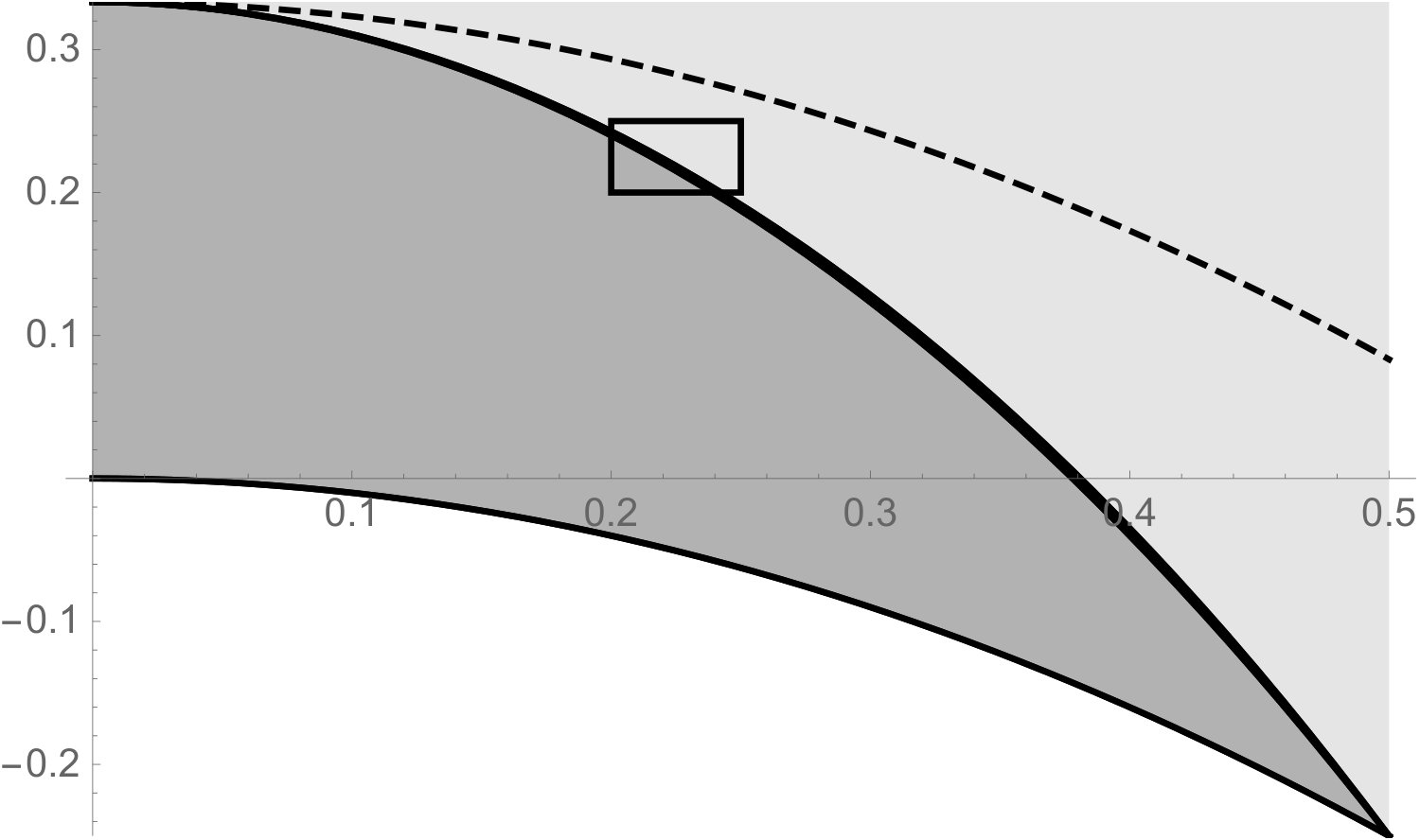 Figure 1
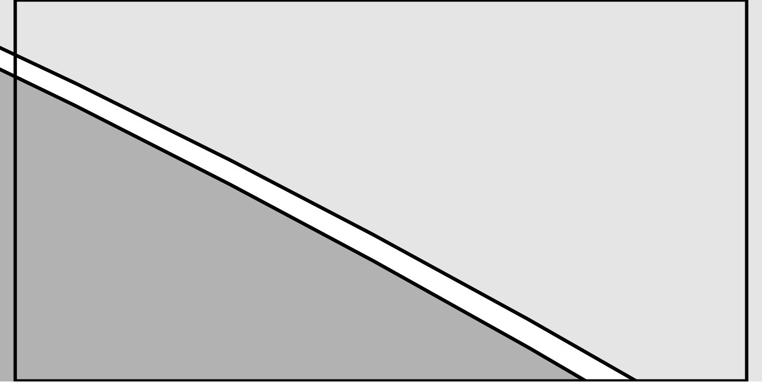 Figure 2
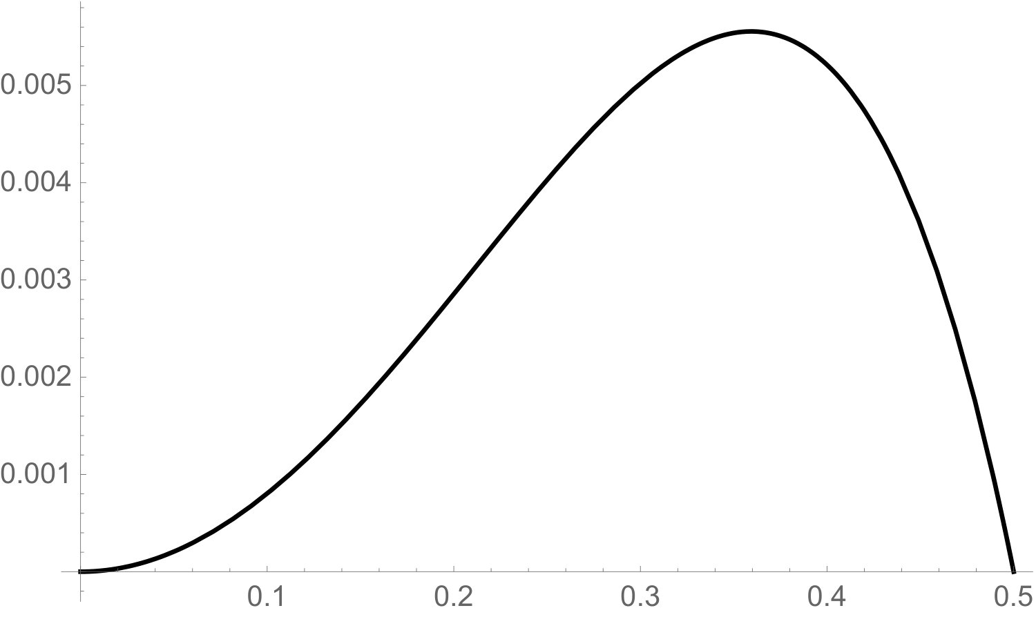 Figure 3
Peer Reviews
No public reviews on file for this paper yet. If you reviewed it on a platform where reviews are public (OpenReview, ICLR, NeurIPS, ICML), you can paste yours below so the community can read it here.
Videos
No videos yet. Explain this paper in a talk, walkthrough, or lecture? Add one.
11institutetext: Département de mathématique, Faculté des sciences, Université Libre de Bruxelles, Campus Plaine CP 213, Bld du Triomphe, B-1050 Brussels, Belgium. E-mail: [email protected]22institutetext: CEREMADE (CNRS UMR n∘ 7534), PSL university, Université Paris-Dauphine, Place de Lattre de Tassigny, 75775 Paris 16, France. E-mail: [email protected] (J.D.), E-mail: [email protected] (M.J.E)33institutetext: Department of Mathematics, Imperial College London, Huxley Building, 180 Queen’s Gate, London SW7 2AZ, UK. E-mail: [email protected]44institutetext: School of Mathematics, Skiles Building, Georgia Institute of Technology, Atlanta GA 30332-0160, USA. E-mail: [email protected]
Symmetry results in two-dimensional inequalities for Aharonov-Bohm magnetic fields
Denis Bonheure
Jean Dolbeault 11
Maria J. Esteban 22
Ari Laptev 22
Michael Loss 3344
Abstract
This paper is devoted to the symmetry and symmetry breaking properties of a two-dimensional magnetic Schrödinger operator involving an Aharonov-Bohm magnetic vector potential. We investigate the symmetry properties of the optimal potential for the corresponding magnetic Keller-Lieb-Thirring inequality. We prove that this potential is radially symmetric if the intensity of the magnetic field is below an explicit threshold, while symmetry is broken above a second threshold corresponding to a higher magnetic field. The method relies on the study of the magnetic kinetic energy of the wave function and amounts to study the symmetry properties of the optimal functions in a magnetic Hardy-Sobolev interpolation inequality. We give a quantified range of symmetry by a non-perturbative method. To establish the symmetry breaking range, we exploit the coupling of the phase and of the modulus and also obtain a quantitative result.
Keywords: Aharonov-Bohm magnetic potential; radial symmetry; symmetry
breaking; magnetic Hardy-Sobolev inequality; magnetic interpolation inequality; optimal constants; magnetic Schrödinger operator; magnetic rings; Caffarelli-Kohn-Nirenberg inequalities; Hardy-Sobolev inequalities.
Mathematics Subject Classification (2010): Primary: 81Q10, 35Q60; Secondary: 35Q40, 81V10, 49K30, 35P30, 35J10, 35Q55, 46N50, 35J20.
1 Introduction and main results
It is a basic question in the calculus of variations whether an optimizer possesses the same symmetries as the minimized functional. The answer depends very much on the details of the functional. The only examples where a general theory is available are linear variational problems where the optimizers are eigenfunctions and hence belong to an irreducible representation of the symmetry group.
Apart when uniqueness is known, for instance in strictly convex problems, it is very difficult to determine whether the minimizer of a non-linear functional is symmetric or whether the symmetry is broken. Symmetry breaking can be shown by minimizing the functional in the class of symmetric functions and then by considering the second variation around this state. If the resulting quadratic form has a negative eigenvalue, then the symmetry is broken. Such a computation can be a formidable problem since it requires quite a bit of information about the minimizer in the symmetric class. Thus, at least in principle, there is a systematic method for proving symmetry breaking. Needless to say, the positivity of the lowest eigenvalue only indicates the stability of the minimizer in the symmetric class but has no bearing on the symmetry of the true minimizer. In general, if the symmetry of the true minimizer is broken, then it does not belong to an irreducible representation of the symmetry group, although it may be invariant under a subgroup. It is therefore difficult to describe minimizers whose symmetry is broken.
It should be clear from these remarks that there is no general theory for proving symmetry and one has to consider some basic examples. There has been a number of non-quadratic variational problems such as Sobolev-type and Hardy-Littlewood-Sobolev inequalities for which this question was successfully answered Aubin-76 ; Talenti-76 ; Lieb-83 ; MR1940370 . The techniques relied mostly on rearrangement inequalities that are closely related to the isoperimetric problem. Another interesting class of examples is furnished by the Caffarelli-Kohn-Nirenberg inequalities which display optimizers with symmetry or with broken symmetry, depending on the values of certain parameters Catrina-Wang-01 ; MR2001882 ; Felli-Schneider-03 . The method for determining the symmetry range, however, is entirely different from the above mentioned techniques and proceeds through a flow method MR3570296 ; MR3612700 .
Common to all these problems is that these are functionals acting on scalar, possibly positive functions. A class of problems that does not fit this mould involve external magnetic fields. In this case the wave function, out of necessity, is truly complex valued and hence the Euler-Lagrange equations form a system of partial differential equations. There has been a number of results for constant magnetic fields. L. Erdös in Erdos96 proved symmetry in a Faber-Krahn type inequality and in BONHEURE2018 D. Bonheure, M. Nys and J. Van Schaftingen proved symmetry for some non-linear problems involving small, constant magnetic fields, albeit in a perturbative sense. Some estimates in MR3784917 suggest that symmetry can also be expected in non-perturbative regimes as well. Likewise the ground state of a quantum particle confined to a circle with a non-zero magnetic flux is treated in doi:10.1063/1.5022121 and optimal results for symmetry and symmetry breaking are given there.
In this paper we treat a non-linear problem related to a Hardy inequality due to A. Laptev and T. Weidl. Let us consider an Aharonov-Bohm vector potential
[TABLE]
corresponding to a singular magnetic field of intensity proportional to . It was shown in MR1708811 that
[TABLE]
and that there is no function for which there is equality. The interesting point is that there is no Hardy inequality in two dimensions without magnetic field and a non-trivial magnetic field is therefore crucial for the Hardy inequality to hold.
The main result of this paper is concerned with a generalization of (2) to the magnetic interpolation inequality
[TABLE]
We shall give a range for the parameters , and for which the minimizer is symmetric and compute the minimizer explicitly. We emphasize that this range is quantitative and is not based on perturbation theory. Moreover, we give also a quantitative range for the parameters for which the symmetry is broken, see Theorem 1.2. In the definition of the vector potential , the constant could be replaced by a function , where is the angle in polar coordinates. See Section 2.1.
As mentioned before, the main difficulty is that the function is complex valued, i.e., at least when , it can be written in the form where the phase is non-trivial. In such a context, standard techniques such as symmetrization have shown to be successful only in very particular situations, see e.g. Erdos96 and MR3665549 ; 2018arXiv180506294L . To explain some of the ideas involved, we use polar coordinates and, when does not vanish, write
[TABLE]
By dropping the term involving the inequality effectively reduces to a problem in which the phase depends only on the polar angle. By optimizing over the phase using ideas from doi:10.1063/1.5022121 the problem is then brought into a form that is a particular class of Caffarelli-Kohn-Nirenberg inequalities for which detailed results are known MR3570296 . The symmetry breaking part is more complicated. The chief reason for this is that the term involving has to be taken into account. This leads to a rather involved computation yielding a region for symmetry breaking that, however, is surprisingly close to the complement of the region where symmetry holds. Good control of the interplay between the phase of and its modulus is a key point to obtaining good estimates for the parameter where symmetry breaking occurs.
There are some interesting consequences of this result. The first is a magnetic version of the Keller-Lieb-Thirring inequalities. Let and define the weighted norm
[TABLE]
We denote by the space of measurable functions such that is finite. Our first result is an estimate on the ground state energy of the magnetic Schrödinger operator on and a symmetry result of the corresponding optimal potential . The magnetic Schrödinger energy is
[TABLE]
and is defined as the infimum of on all such that , where denotes the homogeneous space, i.e.,
[TABLE]
Theorem 1.1 (A magnetic Keller-Lieb-Thirring estimate)
Let , and . Then there is a convex monotone increasing function on such that and
[TABLE]
For , there is an explicit value such that the potential
[TABLE]
is optimal for any . On the contrary, for all equality in (4) is achieved only by non-radial functions if for some explicit .
Notice that the definition of uses a weighted norm. Using the transformations , , and that will be discussed in Section 2.1, the case can be reduced to the range . For , we shall see that . Further details on and will be given later. Let be the inverse of and define
[TABLE]
On the interval , the expression of is explicit and it will be established in Section 3.1 that in this case while the computation of the function can be found in Appendix A. If , the constant is given by where solves
[TABLE]
The constant arises from the analysis of the symmetry breaking phenomenon obtained by considering the linear instability of the radial optimal function. It is similar to the analysis performed by V. Felli and M. Schneider in Felli-Schneider-03 for the Caffarelli-Kohn-Nirenberg inequality without magnetic fields (see also Catrina-Wang-01 for earlier results). The corresponding range with magnetic fields is a range of higher magnetic fields. The symmetry range of the parameters corresponds to a weak magnetic field in which the equality case is achieved by radial potentials. The expression of with defined by (5) is also explicit in terms of given below in Theorem 1.2. We refer to Appendix A.2 for details.
Theorem 1.1 has a dual counterpart which is a statement on the magnetic interpolation inequality (3).
Theorem 1.2 (A magnetic Hardy-Sobolev inequality)
Let and . For any , there is an optimal function which is monotone increasing and concave such that (3) holds for any . With the notation of (6), if and equality in (3) is achieved by
[TABLE]
Conversely, if and with
[TABLE]
there is symmetry breaking, that is, the optimal functions are not radially symmetric.
The existence of an optimal function in (3) follows from a concentration-compactness argument as in Catrina-Wang-01 after an Emden-Fowler transformation that will be introduced in Section 2.3. Section 3.1 is devoted to the proof of Theorem 1.1. Theorem 1.1 and Theorem 1.2 are equivalent as we shall see in Section 3.2. The exponents and are such that . The value of is computed in Appendix A.3. Various other computational issues are dealt with in Appendix A, as well as two figures which summarize the ranges of symmetry and symmetry breaking.
2 Preliminary results
2.1 Considerations on the Aharonov-Bohm magnetic field
The magnetic field , where is given by (1), is equal to in the sense of distributions, where denotes Dirac’s distribution at . Let us consider polar coordinates , so that , , and therefore . On , we consider the uniform probability measure
[TABLE]
We observe that for more general Aharonov-Bohm magnetic fields, could depend on . However, by the change of gauge
[TABLE]
where is the magnetic flux, we notice that
[TABLE]
In this paper we shall therefore always assume that is a constant function without loss of generality.
For any , if , then
[TABLE]
Similarly, if , we find that
[TABLE]
It is therefore enough to consider the case . The general case is obtained by replacing with in all estimates.
2.2 Magnetic kinetic energy: some estimates
Note that when we consider functions depending only on , all integrals on are computed with respect to the probability measure . Our first result is inspired by (doi:10.1063/1.5022121, , Lemma III.2).
Lemma 1
Assume that and is such that . Then we have
[TABLE]
where . Equality holds if and only if and
[TABLE]
In the special case when does not depend on , equality in (8) is achieved if and only if is constant.
Proof
Let be such that . We compute
[TABLE]
After dropping the term , we can optimize
[TABLE]
over the phase using the corresponding Euler-Lagrange equation
[TABLE]
This means that for some . We integrate this identity over and take into account the periodicity of : for some , we have
[TABLE]
In order to minimize the magnetic kinetic energy, we have to choose the best possible and obtain
[TABLE]
As a consequence, the expression of is given by in the equality case in (8) and if does not depend on . On the other hand, equality in (8) is achieved if and only if . ∎
Lemma 2
For all and with , we have
[TABLE]
Proof
First assume that is strictly positive in . With , we can write
[TABLE]
We use the same arguments as in the proof of Lemma 1 and the inequality
[TABLE]
proved by P. Exner, E. Harrell and M. Loss in (MR1708787, , Section IV) to write
[TABLE]
Next let us consider the case when is equal to [math] at some point of . Without loss of generality we can assume that and use the diamagnetic inequality and Poincaré’s inequality applied to in order to obtain
[TABLE]
∎
2.3 Magnetic Hardy and non-magnetic Hardy-Sobolev inequalities
In dimension , the magnetic Hardy inequality (2) holds, as was proved in MR1708811 . When , we notice that .
The weighted interpolation inequality
[TABLE]
is known in the literature as the Caffarelli-Kohn-Nirenberg inequality according to Caffarelli-Kohn-Nirenberg-84 but was apparently discovered earlier by V.P. Il’in, see Ilyin . The exponent is determined by the scaling invariance, the inequality can be extended by density to a space larger than the space of smooth functions with compact support, and as varies in , the parameters and are such that
[TABLE]
Moreover, it is also possible to consider the case in an appropriate functional space after a Kelvin-type transformation: see Catrina-Wang-01 ; DELT09 , but we will not consider this case here. As noticed for instance in DELT09 , by considering , Ineq. (9) is equivalent to the Hardy-Sobolev inequality
[TABLE]
By linear instability, see Felli-Schneider-03 , the optimal functions for (9) are not radially symmetric if . The main ingredient of the proof is reproduced in Appendix A.2, in the two-dimensional case. On the contrary, if , we learn from MR3570296 that equality in (9) is achieved by
[TABLE]
up to a scaling and a multiplication by a constant. In the range , this provides us with the value of the optimal constant, namely where the expression of is given in Appendix A.1. We observe that for any given , we have that , so that the inequality does not make sense for . Using polar coordinates , the Emden-Fowler transformation
[TABLE]
turns Ineq. (10) into
[TABLE]
with . We refer to 1703 for a more detailed review on the Caffarelli-Kohn-Nirenberg inequality. For any given , we define
[TABLE]
so that is the optimal constant in (13) restricted to symmetric functions, that is, functions depending only on . See Appendix A.1 for the explicit expression of . For our purpose, we have to consider a slightly more general problem. For any , let us define
[TABLE]
Lemma 3
Let , and . Then has a minimizer such that and depends only on if and only if
[TABLE]
Proof
The existence of a minimizer is obtained as in the standard case corresponding to and we refer to MR2966111 for the details. The function , where is defined by (11), is a critical point of such that and is linearly instable if and only if (see Appendix A.2). By adapting (MR3570296, , Corollary 1.3), the minimizer of is independent of the angular variable if and only if . In that case, we have for some . ∎
3 Proofs
3.1 Magnetic interpolation inequalities
We prove Theorem 1.2. For more readability, we split the proof into three steps.
Step 1 – Ineq. (3) without the optimal constant. Let . From the diamagnetic inequality, we get
[TABLE]
where , and therefore,
[TABLE]
Using (2) and (10) applied with , such that , this estimate proves the existence of a positive constant in (3). As an infimum on of affine non-decreasing functions of , the function is concave and non-decreasing.
Step 2 – Optimal estimate in the symmetry range. With , and , we know from Lemma 2 that
[TABLE]
We can estimate the optimal constant in (3) by the optimal constant in the relaxed inequality
[TABLE]
Using the Emden-Fowler transformation (12), this inequality can be rewritten on the cylinder as
[TABLE]
By Lemma 3 applied with and , the optimal function for the above inequality is independent of the angular variable if and only if
[TABLE]
that is, with defined by the equality case, i.e., by (6). If , note that there is no such that . With and defined by (6), this amounts to . In that case the optimal function is
[TABLE]
up to a multiplication by a constant and a translation (in the variable). This determines the value of . By construction, we know that , but using as a test function in (3), we find that if . See Appendix A.2 for details on the computation of .
Step 3 – The symmetry breaking range. This range is the set of and for which the optimal functions are not symmetric functions. Let
[TABLE]
We produce a direction of instability for by perturbing the phase and the modulus of simultaneously. Let us start by some preliminary computations. Define , and . An integration by parts shows that
[TABLE]
On the other hand, using the identity , we obtain that
[TABLE]
With the choice corresponding to the optimal constant achieved by the symmetric function , with , by considering \psi_{\varepsilon}(r,\theta):=\big{(}w_{\star}(s)+\varepsilon\,\varphi(s,\theta)\big{)}\,\exp\big{(}i\,\varepsilon\,\chi(s,\theta)\big{)}, at order we obtain that where is the quadratic form defined by
[TABLE]
and
[TABLE]
With the ansatz
[TABLE]
where is a parameter to be fixed later, we obtain that
[TABLE]
with . We minimize the expression of with respect to , that is, we take
[TABLE]
After replacing , , , and by their values in terms of , and , we find that the infimum of the admissible parameters for which is given by (7). Hence we know that there is symmetry breaking for any . This concludes the proof of Theorem 1.2. ∎
Remark 1
The function used in Step 3 of the proof of Theorem 1.2 to produce a negative direction of variation of is only a test function which couples the modulus and the phase. To get an optimal range with this method, one should identify the lowest eigenvalue in the system associated with the variation of : see Section A.4 for details. This is so far an open question as the corresponding eigenfunctions are not identified yet.
One may wonder if a better result could be achieved by varying only the modulus using the function and choosing the optimal . In that case, the instability is reduced to the instability of as defined by (15) with and , which is the classical computation of Felli-Schneider-03 (also see Appendix A.2): here instability occurs if
[TABLE]
Elementary considerations show that and that the threshold given by is by far better (see Fig. 1).
3.2 Spectral estimates
The proof of Theorem 1.1 is a simple consequence of the estimate
[TABLE]
by Hölder’s inequality, with . With the notation , Eq. (4) is a consequence of Eq. (3) in Theorem 1.2: the right-hand side is bounded from below by .
Reciprocally Theorem 1.2 follows from Theorem 1.1 with , which corresponds to the equality case in the above Hölder inequality. ∎
Appendix A Appendix
A.1 Optimal constants in the symmetric case
It is known from zbMATH02502560 that
[TABLE]
is the optimal constant in the inequality
[TABLE]
For any given , the optimal constant in (13) is also in the particular case of symmetric functions, because is the uniform probability measure on . See for instance delPino20102045 for details.
The optimal constants in (10) and (13) are related by (14). In the symmetry range, we have , where
[TABLE]
This expression can be recovered by writing that the equality case in (10) is achieved by the function . Indeed, with the change of variables with and as in (MR3570296, , Section 3.1), and , this means that
[TABLE]
where is the Aubin-Talenti function .
A.2 Ground state eigenvalues of the quadratic form
Linearization and eigenvalues: the one-dimensional case
Let us summarize some classical results on the linearization of the Gagliardo-Nirenberg inequalities in the one-dimensional case, based on (0951-7715-27-3-435, , Appendix A.2). According, e.g., to Dolbeault06082014 , the function is the unique positive solution of
[TABLE]
on , up to translations. The function solves
[TABLE]
With and , is given by
[TABLE]
and solves
[TABLE]
The ground state energy of the Pöschl-Teller operator
[TABLE]
is characterized as follows. The function
[TABLE]
solves
[TABLE]
and therefore provides the principal eigenvalue of ,
[TABLE]
The Sturm-Liouville theory guarantees that generates the ground state.
The lowest non-radial mode on the cylinder
Let us consider the operator
[TABLE]
on the cylinder . By separation of variables, the lowest non-symmetric eigenvalue is associated with the function , so that the ground state of is
[TABLE]
Lowest eigenvalues and threshold for the linear instability
Whenever the optimal function in (3) is radially symmetric, we get that with , i.e., , or
[TABLE]
With defined by (15), let us consider a Taylor expansion of with at order two with respect to . For small enough, the sign of is determined by the sign of the quadratic form
[TABLE]
Hence can be made negative by choosing , which shows that is an instable critical point of if and only if . Notice that Lemma 3 states the reverse result, which is the difficult part of the result: whenever , the minimum of is achieved by so that .
Applied with and , we recover the computation of Felli-Schneider-03 , which determines as in (17). Applied with and , we obtain that
[TABLE]
and observe that it is negative if and only if
[TABLE]
Using in the symmetry range, we obtain that \mu_{\star}(a)=\mu\big{(}\lambda_{\star}(a)\big{)} with given by (18), i.e.,
[TABLE]
A.3 Computation of
Let us give some details on the computation of . An expansion of as defined in Section 3.1 computed with the ansatz (16) shows that it has the sign of
[TABLE]
Since \mathsf{q}(\lambda_{\star})=\big{(}\frac{8\,a}{p^{2}-4}\big{)}^{2}\,(1-4\,a^{2}) is positive for any and since , we know that defined by is such that . Notice that the other root of is in the range , and that the discriminant is positive for any . Additionally, we obtain by direct computation that
[TABLE]
is positive for any . Numerically this difference turns out to be very small: see Figs. 1 and 2.
A.4 The range of linear instability of the magnetic interpolation inequality
The high level of accuracy shown in Fig. 2 deserves some comments. For any given , the threshold between the symmetry region and the symmetry breaking region is in the interval . Since is determined by the choice of (16), one has to understand why this test function gives such a precise estimate.
Let us consider an ansatz in which only the angular dependence is fixed. With
[TABLE]
and the change of variables
[TABLE]
the computation of is reduced to the computation of
[TABLE]
using
[TABLE]
We recover the expression of with the choice
[TABLE]
after optimizing on . All computations done, the optimal value of is
[TABLE]
and we find that for in the admissible range if and only if .
A minimization of under the constraint
[TABLE]
reduces the problem to the identification of the ground state energy in the eigenvalue problem
[TABLE]
For given , the linear instability range is the set of the parameters for which is negative. We know that
[TABLE]
but we do not even know whether is an interval or not. Notice that for , we find that and is a good test function for any : this means that there is symmetry breaking for any .
Acknowledgments
This research has been partially supported by the project EFI, contract ANR-17-CE40-0030 (D.B., J.D.) of the French National Research Agency (ANR), by the NSF grant DMS-1600560 (M.L.), and by the PDR (FNRS) grant T.1110.14F and the ERC AdG 2013 339958 “Complex Patterns for Strongly Interacting Dynamical Systems - COMPAT” grant (D.B.). The authors thank the referees for a careful reading which helped to remove some typos and improve the notations.
© 2019 by the authors. This paper may be reproduced, in its entirety, for non-commercial purposes.
The reference list from the paper itself. Each links out to its DOI / PubMed record.
- 1(1) T. Aubin , Problèmes isopérimétriques et espaces de Sobolev , J. Differential Geometry, 11 (1976), pp. 573–598.
- 2(2) D. Bonheure, M. Nys, and J. Van Schaftingen , Properties of ground states of nonlinear Schrödinger equations under a weak constant magnetic field , J. Math. Pures Appl. (9), 124 (2019), pp. 123–168.
- 3(3) T. Boulenger and E. Lenzmann , Blowup for biharmonic NLS , Ann. Sci. Éc. Norm. Supér. (4), 50 (2017), pp. 503–544.
- 4(4) L. Caffarelli, R. Kohn, and L. Nirenberg , First order interpolation inequalities with weights , Compositio Math., 53 (1984), pp. 259–275.
- 5(5) F. Catrina and Z.-Q. Wang , On the Caffarelli-Kohn-Nirenberg inequalities: sharp constants, existence (and nonexistence), and symmetry of extremal functions , Comm. Pure Appl. Math., 54 (2001), pp. 229–258.
- 6(6) M. Del Pino and J. Dolbeault , Best constants for Gagliardo-Nirenberg inequalities and applications to nonlinear diffusions , J. Math. Pures Appl. (9), 81 (2002), pp. 847–875.
- 7(7) M. del Pino, J. Dolbeault, S. Filippas, and A. Tertikas , A logarithmic Hardy inequality , Journal of Functional Analysis, 259 (2010), pp. 2045 – 2072.
- 8(8) J. Dolbeault and M. J. Esteban , Extremal functions for Caffarelli-Kohn-Nirenberg and logarithmic Hardy inequalities , Proc. Roy. Soc. Edinburgh Sect. A, 142 (2012), pp. 745–767.