Volumetric Spline Parameterization for Isogeometric Analysis
Maodong Pan, Falai Chen, Weihua Tong

TL;DR
This paper introduces a three-stage volumetric spline parameterization method for complex 3D domains that ensures bijectivity and minimal distortion, advancing isogeometric analysis capabilities.
Contribution
A novel three-stage approach combining harmonic maps, max-min optimization, and MIPS to produce high-quality, bijective volumetric parameterizations for complex domains.
Findings
Produces bijective parameterizations with low distortion
Effective for complex 3D domains
Outperforms some existing methods in quality
Abstract
Given the spline representation of the boundary of a three dimensional domain, constructing a volumetric spline parameterization of the domain (i.e., a map from a unit cube to the domain) with the given boundary is a fundamental problem in isogeometric analysis. A good domain parameterization should satisfy the following criteria: (1) the parameterization is a bijective map; and (2) the map has lowest possible distortion. However, none of the state-of-the-art volumetric parameterization methods has fully addressed the above issues. In this paper, we propose a three-stage approach for constructing volumetric parameterization satisfying the above criteria. Firstly, a harmonic map is computed between a unit cube and the computational domain. Then a bijective map modeled by a max-min optimization problem is computed in a coarse-to-fine way, and an algorithm based on divide and conquer…
Click any figure to enlarge with its caption.
 Figure 1
 Figure 2
 Figure 3
 Figure 4
 Figure 5
 Figure 6
 Figure 7
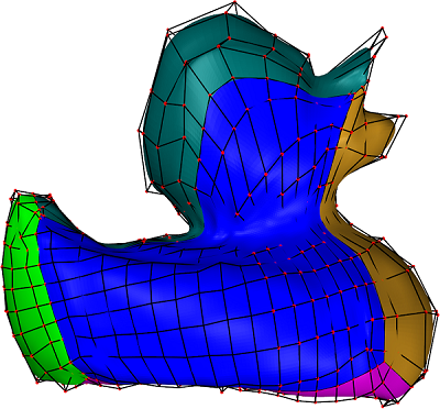 Figure 8
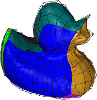 Figure 9
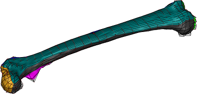 Figure 10
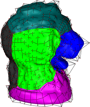 Figure 11
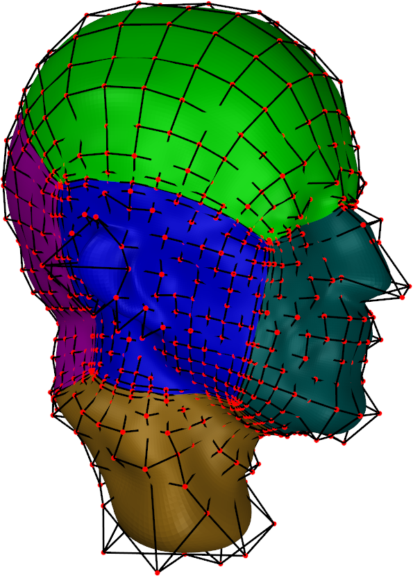 Figure 12
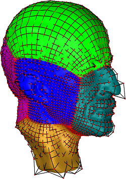 Figure 13
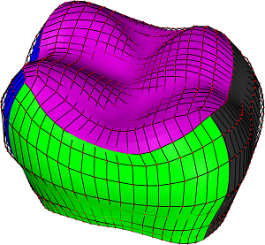 Figure 14
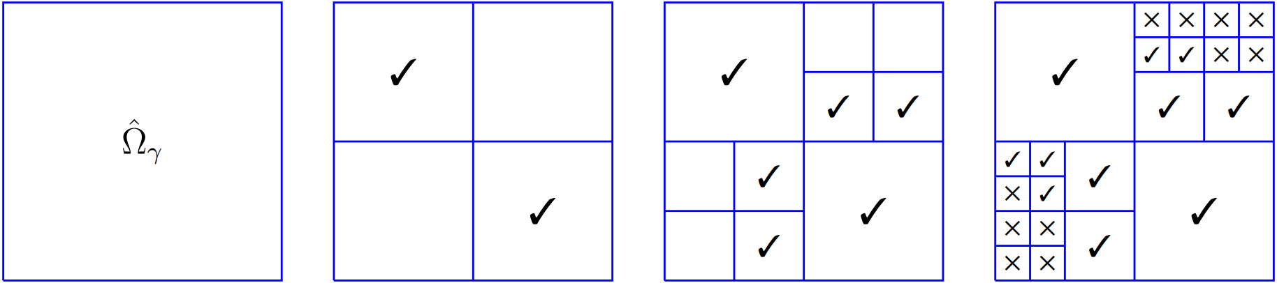 Figure 15
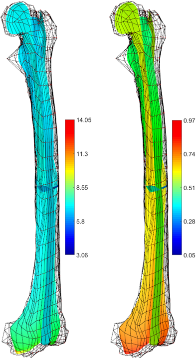 Figure 16
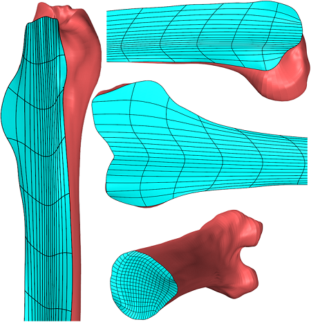 Figure 17
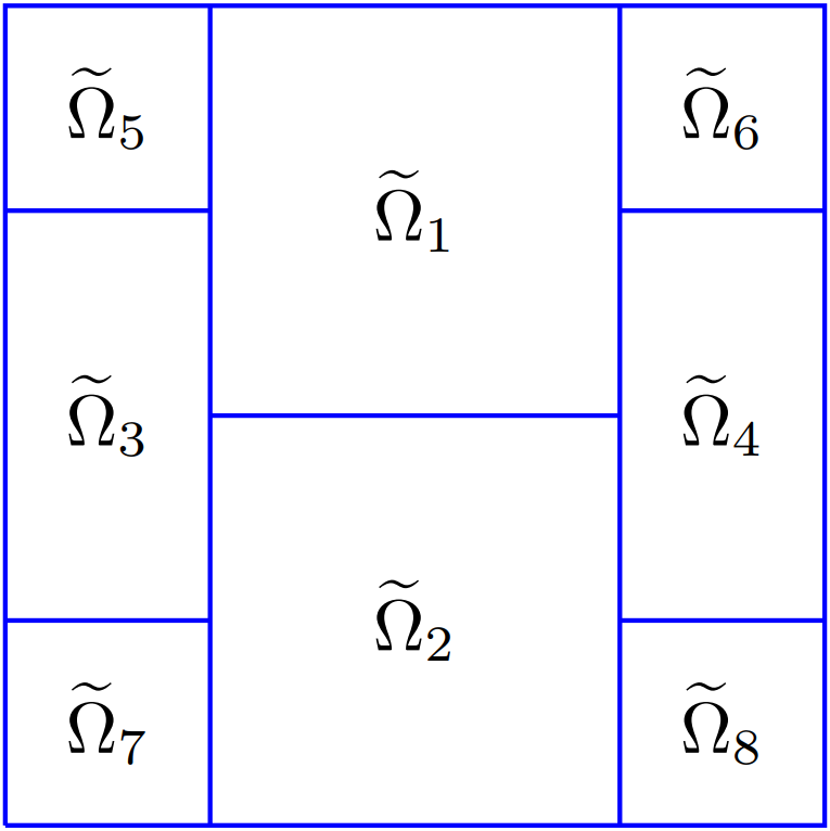 Figure 18
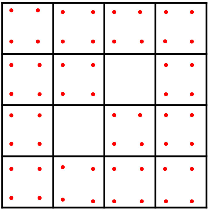 Figure 19
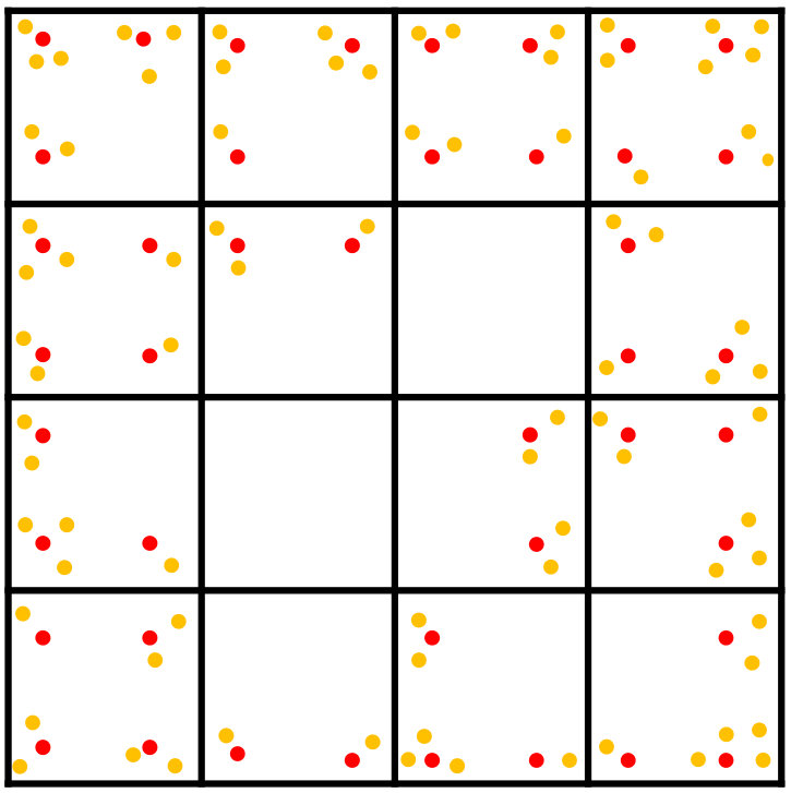 Figure 20
 Figure 21
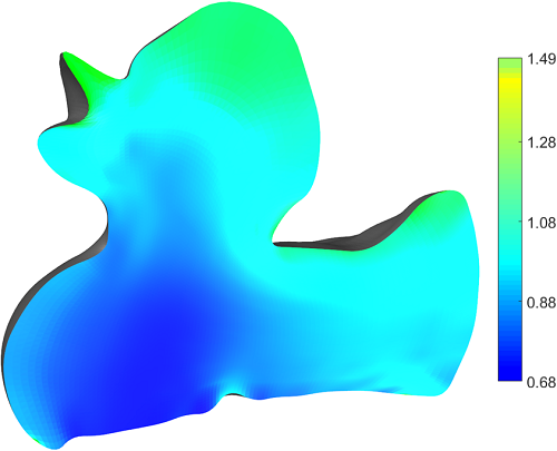 Figure 22
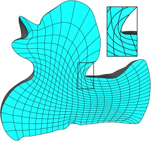 Figure 23
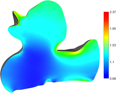 Figure 24
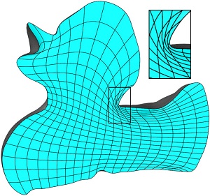 Figure 25
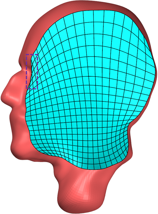 Figure 26
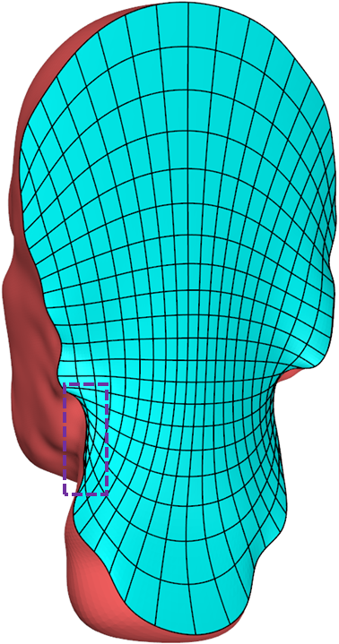 Figure 27
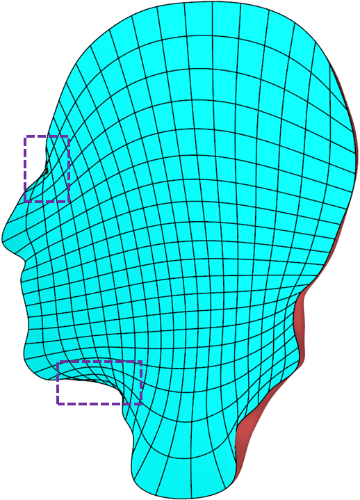 Figure 28
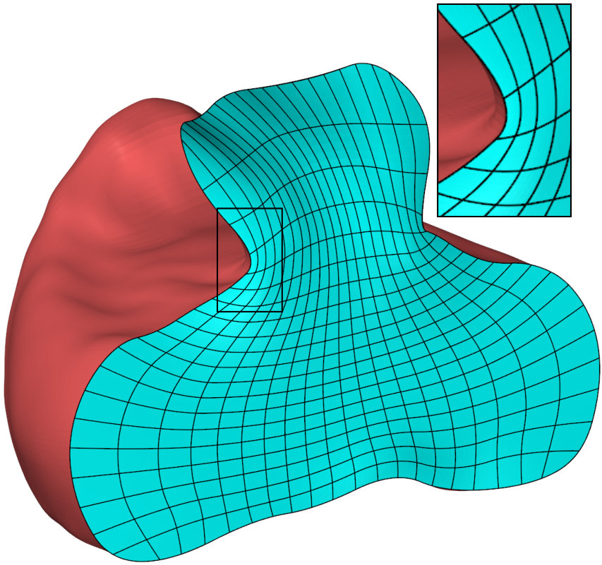 Figure 29
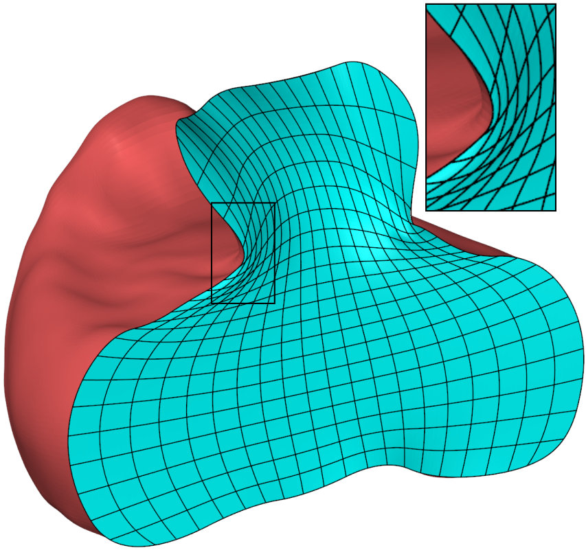 Figure 30
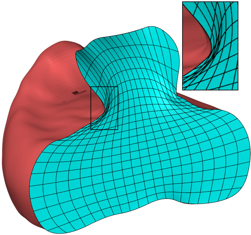 Figure 31
 Figure 32
 Figure 33
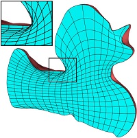 Figure 34
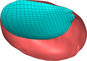 Figure 35
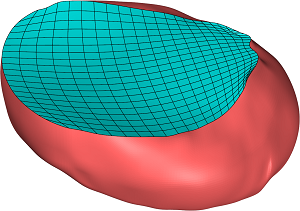 Figure 36
 Figure 37
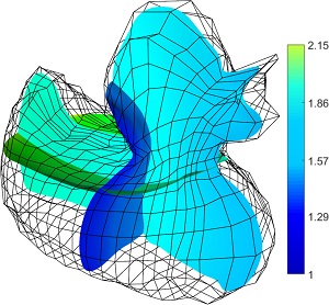 Figure 38
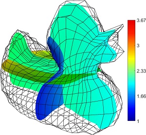 Figure 39
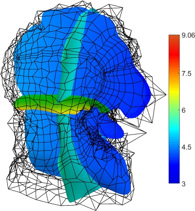 Figure 40
| Model | , , , , , | Method | , , , , | Time (m) |
| Tooth Fig. 9 | 20, 20, 7, 3, 3, 3 | Xu’s | 63.61, 0.01, 0.90, 0.04, 6.06 | 8.43 |
| Wang’s | 46.77, 0.01, 0.93, 0.19, 6.96 | 7.04 | ||
| Ours | 9.50, 0.10, 0.99, 0.24, 5.66 | 3.31 | ||
| Duck Fig. 10 | 17, 7, 11, 2, 2, 2 | Xu’s | , 0.00, 0.97, -4.36, 21.58 | 10.25 |
| Wang’s | 56.37, 0.00, 0.98, 0.04, 6.98 | 5.18 | ||
| Ours | 10.94, 0.01, 0.99, 0.17, 7.15 | 6.62 | ||
| Lion Fig. 11 | 17, 17, 17, 3, 3, 3 | Xu’s | — | — |
| Wang’s | , 0.00, 0.98, -0.52, 10.85 | 24.51 | ||
| Ours | 9.06, 0.09, 0.99, 0.14, 11.07 | 16.35 | ||
| Femur Fig. 12 | 29, 13, 9, 2, 2, 2 | Xu’s | — | — |
| Wang’s | , 0.02, 0.97, -1.96, 11.03 | 15.88 | ||
| Ours | 14.05, 0.05, 0.97, 0.12, 10.18 | 23.14 | ||
| Max Planck Fig. 13 | 24, 24, 24, 3, 3, 3 | Xu’s | — | — |
| Wang’s | 17.53, 0.03, 0.98, 0.09, 10.36 | 39.79 | ||
| Ours | 8.88, 0.07, 0.99, 0.14, 8.29 | 21.76 |
Peer Reviews
No public reviews on file for this paper yet. If you reviewed it on a platform where reviews are public (OpenReview, ICLR, NeurIPS, ICML), you can paste yours below so the community can read it here.
Videos
No videos yet. Explain this paper in a talk, walkthrough, or lecture? Add one.
Volumetric Spline Parameterization for Isogeometric Analysis
Maodong Pan
Falai Chen
Weihua Tong
School of Mathematical Sciences, University of Science and Technology of China, Hefei, Anhui, 230026, PR China
Abstract
Given the spline representation of the boundary of a three dimensional domain, constructing a volumetric spline parameterization of the domain (i.e., a map from a unit cube to the domain) with the given boundary is a fundamental problem in isogeometric analysis. A good domain parameterization should satisfy the following criteria: (1) the parameterization is a bijective map; and (2) the map has lowest possible distortion. However, none of the state-of-the-art volumetric parameterization methods has fully addressed the above issues. In this paper, we propose a three-stage approach for constructing volumetric parameterization satisfying the above criteria. Firstly, a harmonic map is computed between a unit cube and the computational domain. Then a bijective map modeled by a max-min optimization problem is computed in a coarse-to-fine way, and an algorithm based on divide and conquer strategy is proposed to solve the optimization problem efficiently. Finally, to ensure high quality of the parameterization, the MIPS (Most Isometric Parameterizations) method is adopted to reduce the conformal distortion of the bijective map. We provide several examples to demonstrate the feasibility of our approach and to compare our approach with some state-of-the-art methods. The results show that our algorithm produces bijective parameterization with high quality even for complex domains.
keywords:
Volumetric parameterization, isogeometric analysis, max-min optimization, MIPS.
1 Introduction
Isogeometric analysis (IGA) has recently become a hotspot in numerical analysis and geometric modeling communities since it integrates two related disciplines: Computer Aided Design (CAD) and Computer Aided Engineering (CAE) [14]. IGA overcomes the unnecessary data exchange between CAD models and the simulation software, and it has been successfully applied in various disciplines, such as structural vibration [6], shell analysis [2], phase transition phenomena [11] and shape optimization [29, 23].
However, CAD systems provide only the boundary representation of an object (computational domain), while CAE typically requires the interior parameterization of the object. Thus constructing a volume parametric representation for the computational domain from the given boundary data is an essential step in IGA, and it is called volumetric parameterization (see Fig. 1). Volumetric parameterization has great effect on the accuracy and efficiency in subsequent analysis [5, 40, 28, 45]. As sated in [8, 39, 27], a good volumetric parameterization should meet two basic requirements: firstly, it doesn’t have self-intersections, i.e., the map from the parametric domain (generally a unit cube) to the computational domain is injective; secondly, the distortion of the map should be as small as possible, i.e., the volumes and angles after mapping should be preserved as much as possible. So far several approaches have been proposed to solve the volumetric parameterization problem, and they can be generally classified into two categories: (1) volumetric spline parameterization from boundary triangulations [20, 7, 46, 35, 17]; and (2) analysis-suitable volumetric parameterization from spline boundaries [1, 24, 47, 42, 41, 43, 44, 36, 19]. However, none of these methods have fully addressed the above issues. For example, no method guarantees the bijectivity of the parameterization, especially for complex computational domains. Thus constructing high-quality volumetric parameterizations of complex computational domains remains a big challenge in IGA.
This paper describes a new approach for constructing high-quality volumetric parameterization. Specifically, suppose we are given the six spline boundary surfaces of a computational domain (of genus-zero), our goal is to construct a trivariate spline representation for the computational domain such that the parameterization is bijective and has low distortion. We propose a three-stage approach to solve the problem. Firstly, an initial parameterization is obtained by computing a harmonic map from the parametric domain (a unit cube) to the computational domain. Then we compute a bijective parameterization of the computational domain by solving a max-min optimization problem in a coarse-to-fine way. Finally, we improve the parameterization quality by minimizing the conformal distortion of the map using the MIPS method.
The remainder of this paper is organized as follows. Section 2 reviews some related work about domain parameterization. Section 3 presents some preliminary knowledge about the representation of volumetric parameterization, the sufficient condition for an injective parameterization and the distortion measurement of a parametrization which will be used in our method. In Section 4, we propose three mathematical models followed by algorithms to compute a high-quality map for volumetric parameterization. Some examples are demonstrated in Section 5 to show the effectiveness of the proposed method, and comparisons with the nonlinear optimization methods [41, 36] are also provided. Finally, we conclude the paper with a summary and future work in Section 6.
2 Related work
In this section, we will review some related works on domain parameterization and emphasis will be put on volumetric parameterization.
For planar domain parameterization, a direct solution is the discrete Coons patches introduced by Farin and Hansford [9]. Gravesen et al. [12] put forward a spring model to solve the problem. These two methods are simple but the resulting parameterization may not be injective. To ensure a bijective parameterization, several approaches were proposed by solving nonlinear optimization problems [40, 25, 32]. For complex computational domains, however, single patch representations do not provide sufficient flexibility, and multi-patch structures were put forward to tackle the parameterization problem [45, 3, 39, 38]. Recently, Juettler et al. [15] and Pan et al. [27] investigated the low-rank parameterization of planar domains which can improve the efficiency of assembling stiffness matrices in IGA.
Compared with planar case, volumetric parameterization is more challenging. Depending on the boundary representation (triangular meshes or splines) of a 3D computational domain, volumetric parameterizaion methods can be classified into two categories. For a domain whose boundary is represented by triangular meshes, Martin et al. [20] proposed a trivariate B-spline parameterization method based on discrete volumetric harmonic functions. In [7], the authors focused on constructing a solid T-spline from the parametric mapping of tetrahedral meshes generated by meccano method from the input surface mesh. Zhang et al. [46] developed a procedure to construct a T-spline representation of a genus-zero solid. When the computational domain has a topology of non-zero genus, polycube is a useful tool to solve the parameterization problem [16, 33, 34]. To extend the work [46] to domains with arbitrary topology, Wang et al. [35] used the polycube mapping combined with subdivision and pillowing techniques to generate high-quality T-spline representations. Inspired by CSG Boolean operations, Liu et al. [17] firstly built the polycubes from the input triangle mesh based on Boolean operations and then computed the volumetric parameterization by performing an octree subdivision on the polycubes. Later on skeleton-based polycube constructions were used to generate T-spline parameterizations [18]. For computational domains with spline boundary representations, Aigner et al. [1] presented a method for generating NURBS parameterizations of swept volumes via sweeping a closed curve. Nguyen et al. [24] applied a sequence of harmonic maps to construct a volumetric parameterization, and the harmonic maps were obtained by solving some variational problems. In [47], the construction of volumetric conformal T-spline parameterization from boundary T-spline representation was studied by using octree structure and boundary offset. An optimization-based method was proposed in [41], where the B-spline parameterization is found by solving a constraint optimization problem. A similar technique was proposed by the same authors in [42]. From six boundary B-spline surfaces, Wang and Qian [36] proposed an efficient method by combining the constraint aggregation and hierarchical optimization technique to obtain valid trivariate B-spline solids. Recently, a method based on a new T-mesh untangling and smoothing procedure was proposed to construct T-spline parameterizations for 2D and 3D geometries [19].
Despite various methods for volumetric parameterization were proposed, however to the best of our knowledge, none of the methods can ensure the bijectivity of the parameterization, and the quality of the parameterization is not well investigated. The goal of the current paper is to present a new volumetric parameterization technique which can guarantee the bijectivity of the parameterization and has lowest possible distortion.
3 Preliminaries
In this section, we present some preliminary knowledge about the representation of volumetric parameterizations, the sufficient condition for a bijective parameterization and the distortion measurement of a parameterization.
3.1 Representation of volumetric parameterization
In this paper, we assume a simply connected computational domain is parameterized by a vector-valued trivariate tensor product B-spline function:
[TABLE]
where are the control points, , and are the B-spline basis functions of degree , and w.r.t the knot sequences , and in respectively. defines a tensor product mesh over which the B-spline function is a piecewise polynomial, i.e, is a polynomial over each cell (a cube) of the mesh .
3.2 Sufficient condition for a bijective parameterization
To guarantee the bijectivity of a map, a necessary condition is the positivity of the Jacobian of the map. In general, we have
Lemma 1**.**
([21]) A continuously differential map is locally bijective provided its Jacobian, denoted as , does not vanish on the parametric domain, and the global bijectivity of is guaranteed if it is locally bijective on the parametric domain, and the computational domain is simply connected and the restriction of on the domain boundary is bijective.
In this work, we always assume that the computational domain is simply connected, and a bijective boundary correspondence of the parametric domain and computational domain is established. Thus in this case, a locally bijective parameterization is also globally bijective.
From Lemma 1, it is obvious that if the Jacobian is positive everywhere on the parametric domain, i.e.,
[TABLE]
then the parametrization is globally bijective.
Owning to the good properties of B-splines [22], the Jacobian of a volumetric B-spline parameterization (1) is itself a higher order trivariate B-spline which has the following form:
[TABLE]
where denote the coefficients of the higher order B-spline. From the convex hull property of B-spline function, a sufficient condition for the bijectivity of the parameterization (1) is that all the coefficients are positive. However, this is a very strict condition for a bijective parameterization as reported in [43]. In order to relax the condition, we convert the B-spline representation (3) into Bézier forms:
[TABLE]
where are the control coefficients, , and denote the Bernstein basis polynomials of degree , and respectively, and is a cell of the tensor product mesh . The coefficients of these trivariate Bézier polynomials can be obtained by multiple knot insertion using the blossoming technique [10]. Now if all the coefficients are positive, then the Jacobian is also positive on the parametric domain . On the other hand, if some coefficients in are negative, we can further subdivide the Bézier polynomial into eight sub-polynomials at the parametric values and check the positivity of the coefficients of each sub-polynomial. Again if the coefficients of all the Bézier polynomials (including polynomials after subdivision) are positive, the Jacobian is also positive. This process can be repeated until certain level of subdivisions. In this way, we can obtain a set of relaxed sufficient conditions for the bijectivity of the map . However, a risk of such process is that the number of inequality constraints will be huge [39].
Instead of using the above sufficient conditions as constraints, in this paper we will directly impose positivity constraints of the Jacobian at a set of collocation points, and apply the above sufficient conditions to check the positivity of the Jacobian on the whole parametric domain .
3.3 The distortion measurement of a parameterization
The distortion of a differentiable map at a point is some measure about how changes at the vicinity of . Here we introduce two common measures of distortion: volume distortion and conformal (angular) distortion. In addition, the fairness measure for a map is also introduced.
Volume distortion. The volume distortion is the determinant of the Jacobian of the map divided by the volume of :
[TABLE]
Thus is also called the scaled Jacobian of the map . The optimal map is the one that satisfies everywhere.
Conformal distortion. A conformal map preserves angles and thus it can produce iso-parametric orthogonal nets. Denote the singular values of as , and , then the conformal distortion can be defined by MIPS function [13]:
[TABLE]
where stands for the Frobenius norm. It’s easy to see that achieves the minimal value if and only if , that is, is a conformal map.
Fairness. Besides that the map should have smallest distortion, we also hope the map is smooth and fair. This can be characterized by the triharmonic quantity:
[TABLE]
where , and are the Hessians of , and respectively.
4 A three-stage parameterization method of computational domains
Given the B-spline representations of the six boundary surfaces of a computational domain , our goal is to compute a trivariate B-spline representation for , i.e., a map from the unit cube to which is bijective and has low distortion. In this section, we introduce a three-stage approach towards the goal.
4.1 Computing a harmonic map
The first stage of our method is to compute a good initial parameterization which is critical for accelerating the convergence of subsequent optimization. There are several ways to construct an initial parameterization such as discrete Coons volumetric interpolation [9] and deformation based method [36]. In this paper, we compute a harmonic map as the initial parameterization. The computation is similar to those in [37, 31] except that our representation is spline-based.
According to the smooth harmonic map theory [30], a harmonic map is a function satisfying Laplace’s equation, i.e.,
[TABLE]
where is the Laplace operator. Thus the harmonic map under the given boundary information can be found by minimizing the following energy
[TABLE]
This is a quadratic optimization problem and the solution can be obtained by solving a sparse and symmetric linear system of equations. The preconditioned conjugate gradient method with incomplete Cholesky factorization is applied in solving the linear system. From Fig. 2, we can see that the initial parameterization constructed using harmonic map is nearly valid (i.e., the parameterization is bijective except at regions near the boundary), which is superior to most of the other initialization methods.
4.2 Construction of a bijective parameterization
With the above constructed harmonic map as the input, the next stage of our method is to compute a bijective parameterization of the computational domain . This is the key step of our algorithm.
4.2.1 Theoretic foundation
To ensure the bijectivity of the parameterization , the sufficient conditions proposed in Section 3.2 were applied by previous literature like [41] and [36]. However, the number of such conditions can be very large, which makes the construction of a bijective parameterization very difficulty.
In this paper, we propose an alternative approach to solve the problem. We maintain a set of collocation points , over which we explicitly monitor and control the bijectivity of , that is,
[TABLE]
Obviously, if the collocation points are dense enough, then the discrete bijectivity constraints (9) can ensure the bijectivity of the map over the whole domain . The theoretic foundation of this idea is based on the following lemma and theorem.
Lemma 2**.**
The determinant of the Jacobian of a map is Lipschitz continuous if
[TABLE]
In fact,
[TABLE]
This lemma can be proved using the mean value theorem and it relates the bijectivity of the map over the parametric domain to the bijectivity on the set of collocation points . Specifically, we have the following theorem.
Theorem 1**.**
Given a set of collocation points and a positive lower bound of the determinant of the Jacobian of the map over , the bijectivity of can be accomplished if the fill distance of the collocation points in satisfies
[TABLE]
where the fill distance is the one-sided Hausdorff distance:
[TABLE]
Proof.
For , such that . According to Lemma 2, we have
[TABLE]
Therefore,
[TABLE]
Thus the conclusion follows by Lemma 1. ∎
4.2.2 Max-min optimization model
Now we propose a mathematical model to compute a bijective map from to :
[TABLE]
where is a thin-plate energy defined as
[TABLE]
which is used to control the fairness of the map. and are two positive thresholds. In our model, we maximize the minimum of the determinants of the Jacobian at the collocation points, which is equivalent to minimize the volume distortion in a sense.
By introducing an auxiliary slack variable , the above max-min optimization problem (11) can be converted into the following optimization problem:
[TABLE]
where is a some free parameter.
Remark 1**.**
If we apply the sufficient conditions described in Section 3.2 as constraints to ensure the bijectivity of the map, then our mathematical takes the similar form:
[TABLE]
where the number of the inequality constraints is generally much larger than , and it is much more than that in the model (11). Table 1 presents a comparison of the number of constraints in the two mathematical models for five examples. The number of constraints in the model (11) is only about one fourth of that by the model (13). Thus our optimization model (11) is much less computationally expensive than the model (13).
4.2.3 A coarse-to-fine parameterization method
A key issue to solve the optimization problem (12) is to select the collocation points appropriately. Too many collocation points introduce too many nonlinear constraints in the optimization problem, and computational complexity of the problem increases tremendously. To accelerate the computational process, we propose a coarse-to-fine strategy with a Jacobian gradient guided selection scheme for the collocation points. Specifically, initialize as the empty set and as the harmonic map computed in Section 4.1, our algorithm repeats the following two steps:
Convert the B-spline representation of into Bézier forms, and for each Bézier polynomial check the positivity of by looking at its Bézier coefficients or those of its subdivided Bézier polynomials (to certain level) as described in Section 3.2. If all the Bézier coefficients are above , then is positive over its defining cell and we remove the collocation points (if any) in from ; otherwise add new collocation points from the cell to . See Figures 3 and 4 for an illustration in 2D case. 2. 2.
Compute a parameterization by solving the problem (12) using the algorithm presented in Section 4.2.4.
The above procedure runs until the parameterization becomes bijective or the level counter reaches the maximal level . The bijectivity of the parameterization is achieved if the bijectivity conditions for all the cells are satisfied.
Over the cell at level , obviously we need only to add the new collocation points in those sub-cells marked with ‘✕’ (see Fig. 3), and these new collocation points are generated based on the gradient of , i.e., more points are needed where the gradient is large while fewer ones where the gradient is small. Specifically, for a sub-cell marked with ‘✕’, denoted as , we firstly uniformly subdivide it into sub-cuboids , (, , ), then the number of new collocation points added to each sub-cuboid can be computed as follows
[TABLE]
where is the value of at the center of , is the maximum value of , is an adjusting positive parameter, and , denote the volumes of , respectively. Fig. 5 illustrates the whole process of our parameterization method.
4.2.4 Numerical algorithm
The optimization problem (12) can be solved by the interior-point algorithm [26] which is effective in solving large-scale nonlinear optimization problems. However, when parameterizing complex domains, the number of variables and constraints in (12) can be very large, ranging from tens to hundreds of thousands. So many variables and constraints are a big burden for solving nonlinear constrained optimization problems. In order to improve the computational efficiency, we apply a divide and conquer strategy to solve the problem (12). Generally speaking, the main idea is to split the parametric domain into several non-overlapping regions and then solve the problem (12) over each subregion separately, and finally combine the solutions over the subregions to constitute the solution of the original problem. Fig. 6 illustrates this approach in 2D case, where the parametric domain is subdivided into eight sub-domains (denoted as , ), and the problem (12) is solved over each sub-domain separately.
Remark 2**.**
In solving the problem (12) at certain level, there is no need to compute those control points of the B-spline parameterization (1) whose influence region is contained in some region marked with ‘✓’, and they are kept unchanged from previous level. The free variables are the control points whose influence region contains the region marked with ‘✕’.
Remark 3**.**
Since B-spline basis functions have local compact supports, only a few variables may contribute to each constraint in (12), i.e., the constraint conditions are sparse in variables. This can greatly reduce the computational complexity in our algorithm.
Remark 4**.**
For two adjacent subregions and , the optimization problem (12) may have common variables. In order to keep these sub-problems separable, we solve them in a certain order, such as from the subregion to , and when a sub-problem is solved, its optimization variables are fixed. However, in some situations, there may be no feasible solutions to the subsequent sub-problems due to the lack of degree of freedom. In this case, a local offset function represented by a linear combination of some B-spline basis functions with more compact supports can be added over the corresponding subregion to achieve a feasible solution.
4.3 Improving parameterization quality using MIPS
In the previous subsection, we designed a mathematical model to construct a bijective parameterization of a three dimensional domain. In that model, only volumetric distortion is considered, and consequently the distortion of the parameterization is a bit large in some concave regions, see for example, Fig. 5(f) and Fig. 7. In this subsection, we further improve the quality of the parameterization map constructed in the previous subsection using MIPS–an efficient global parameterization method which minimizes the conformal distortion of the map [13]. The problem is formulated as
[TABLE]
where is the conformal distortion of introduced in Section 3.3.
To solve the above optimization problem, one first has to discretize the integral using Gaussian quadrature rules. Then the problem can be solved efficiently using the L-BFGS which is a quasi-Newton method for solving unconstrained nonlinear minimization problems [26]. The initial solution is provided by the bijective parameterization computed in the last subsection. The bijectivity of the parameterization can be preserved during the optimization process since MIPS can penalize invalid parameterization. In fact the objective function in (14) goes to infinity when approaches zero. Numerical examples demonstrate that this step of optimization is essential and effective, see Fig. 7 for a comparison.
Now the overall algorithm of our volumetric parameterization is summarized in Algorithm 1.
5 Experimental results
In this section, we apply our volumetric parameterization method to several computational domains, and for each example, the bijectivity and distortion are demonstrated. Furthermore, comparisons with two nonlinear optimization methods [41, 36] are performed. We didn’t compare our method with some other competitive methods [7, 46, 35, 19] since they construct parameterizations from triangle meshes rather than spline boundary surfaces and they utilized T-splines instead of NURBS as the representation of the parameterization. Furthermore, these methods do not guarantee the bijectivity of the parameterization.
5.1 Implementation details
Our method is implemented using C++ with visual studio 2017 on windows 10 platform. The optimization problems (12) and (14) are solved using the Artelys Knitro’s software [4]. All experiments are conducted on a laptop computer of an Intel Core i5-7300HQ CPU, 2.5GHz with 8GB memory. There are several parameters which need to be specified. The knot vectors and the degree of the B-spline representation in (1) are provided in Table 2. In the bijective parameterization model (12), there are two parameters, i.e., and . We typically set . The weight can be used to balance the bijectivity and distortion of the parameterization. Clearly, larger leads to parameterization results of lower distortion while smaller can increase the bijectivity of the parameterization. We observe that provides a good compromise between them.
5.2 Parameterization results
5.2.1 Quality metric for parameterization
We use three metrics—the condition number of the Jacobian matrices, the orthogonality of the iso-parametric elements and the volume distortion of the parameterizaton to evaluate the quality of a parameterization.
The condition number of the Jacobian matrix defined as
[TABLE]
indicates whether the Jacobian matrix is ill-conditioned or not. It’s easy to see that this metric can characterize the conformal distortion of the parameterization by (6).
The orthogonality of iso-parametric structure is also an important quality measure of analysis suitable volumetric parameterization in IGA applications [44], which can be defined according to the differential geometry property of parametric volumes as follows
[TABLE]
Obviously achieves its maximal value if and only if . And the larger is, the more orthogonal the iso-parametric structure of the parameterization is. Again this metric is related with conformal distortion.
Besides the above two metrics, another important criteria to evaluate the quality of the parameterization is the volume distortion (also called as the scaled Jacobian) as described in Section 3.3. In our experiments, to measure the volume distortion of the parameterization, we uniformly partition the parametric domain into sub-cuboids , (, , ), then the volume distortion over the sub-cuboid , denoted as , can be computed as
[TABLE]
where is the volume of .
5.2.2 Parameterization of different computational domains
We demonstrate five examples (as illustrated in Fig. 8) to show the effectiveness of the proposed approach, and some comparisons with Xu’s method [41] and Wang’s method [36] are provided.
Fig. 9 depicts the results of volume parameterization of the tooth model by the three methods. The six given boundary B-spline surfaces are shown in Fig. 8(a). In order to show the parameterization quality, three interior iso-parametric surfaces for Xu’s method, Wang’s method and our method are provided in the first three rows of Fig. 9. The condition number and orthogonality colormaps of these iso-parametric surfaces are shown in the next two rows respectively. In order to verify the volume preserving property of these methods, we calculate the volume distortion distributions, which are illustrated in the last row of Fig. 9. The bijectivity of the parameterization for this model is verified by the criterion described in Section 3.2. From this example it can be seen that our method produces smaller distortion and better orthogonality than the other two methods. Fig. 10 shows the comparison results of the duck model. In this example, we observe that Xu’s method has many self-intersections and the distortion of Wang’s method is a bit large in some concave regions, while our method is always bijective and has lower distortion. Fig. 11 shows the parameterization results of the lion model by Wang’s method and our method. It can bee seen that Wang’s method is not bijective in the extremely concave regions, while our method can still produce bijective parameterization. More results for complex models by our approach are also demonstrated, including the femur model in Fig. 12 and Max Planck model in Fig. 13. In the last three examples (Fig. 11-13), Xu’s method is unable to achieve a valid parameterization in a limited amount of time. From all these examples, we can conclude that the proposed method can achieve high-quality parameterizations and significantly outperforms the other two methods in terms of bijectivity, distortion and orthogonality.
Table 2 summarizes the quantitative results (including distortion, orthogonality and running time) of the examples presented in Fig. 9-13, which also validate that our parameterization method is bijective, achieves lower distortion, better orthogonality and comparable computational efficiency than the other two state-of-the-art methods.
6 Conclusions and future work
Volumetric parameterization of computational domains is an essential step in IGA as mesh generation in finite element analysis. In this work, we propose a novel volumetric parameterization approach which includes three main steps: computing an initial harmonic mapping, constructing a bijective mapping by solving a max-min constrained optimization problem and improving parameterization quality using MIPS. Coarse-to-fine and divide-conquer strategies are applied to efficiently solve the optimization problems. Experimental examples demonstrate that our approach can produce a bijective and low-distortion volumetric parameterization which outperforms other state-of-the-art methods.
Regarding the future work, there are two major problems which are worthy of further investigation. Firstly, the running time reported in Table 2 indicates that our algorithm is still computationally expensive, which may be accelerated by GPU computation. Secondly, currently our approach only deals with geometries of genus-zero. For geometries with high genus and more complex boundaries, the domain decomposition method may have to be applied to partition the domain into simply connected regions and then each region can be parameterized using the technique proposed in this paper.
Acknowledgement
This work was supported by the NSF of China (No. 11571338, 61877056), China Postdoctoral Science Foundation (No. 2018M632548), the Fundamental Research Funds for the Central Universities (No. WK0010460007), and the Open Project Program of the State Key Lab of CADCG (No. A1819), Zhejiang University.
The reference list from the paper itself. Each links out to its DOI / PubMed record.
- 1[1] Aigner, M., Heinrich, C., Jüttler, B., Pilgerstorfer, E., Simeon, B., Vuong, A.-V., 2009. Swept volume parameterization for isogeometric analysis. In: IMA international conference on mathematics of surfaces. Springer, pp. 19-44.
- 2[2] Benson, D., Bazilevs, Y., Hsu, M.-C., Hughes, T., 2011. A large deformation, rotation-free, isogeometric shell. Computer Methods in Applied Mechanics and Engineering 200 (13), 1367-1378.
- 3[3] Buchegger, F., Jüttler, B., 2017. Planar multi-patch domain parameterization via patch adjacency graphs. Computer-Aided Design 82, 2-12.
- 4[4] Byrd, R. H., Nocedal, J., Waltz, R. A., 2006. Knitro: An integrated package for nonlinear optimization. In: Large-scale nonlinear optimization. Springer, pp. 35-59.
- 5[5] Cohen, E., Martin, T., Kirby, R., Lyche, T., Riesenfeld, R., 2010. Analysis-aware modeling: Understanding quality considerations in modeling for isogeometric analysis. Computer Methods in Applied Mechanics and Engineering 199 (5), 334-356.
- 6[6] Cottrell, J. A., Reali, A., Bazilevs, Y., Hughes, T. J., 2006. Isogeometric analysis of structural vibrations. Computer methods in applied mechanics and engineering 195 (41), 5257-5296.
- 7[7] Escobar, J., Cascón, J., Rodríguez, E., Montenegro, R., 2011. A new approach to solid modeling with trivariate t-splines based on mesh optimization. Computer Methods in Applied Mechanics and Engineering 200 (45), 3210-3222.
- 8[8] Falini, A., Špeh, J., Jüttler, B., 2015. Planar domain parameterization with thb-splines. Computer Aided Geometric Design 35, 95-108.