Parametric FEM for Shape Optimization applied to Golgi Stack
Xinshi Chen, Eric Chung

TL;DR
This paper develops a parametric finite element method for shape optimization of Golgi stacks, modeling cisternae as elastic vesicles to understand their morphological evolution.
Contribution
It introduces a novel FEM-based shape optimization model for Golgi stacks, incorporating biological constraints and handling multiple vesicles simultaneously.
Findings
The model successfully simulates Golgi stack shapes.
Numerical results align with observed Golgi morphologies.
The approach offers insights into Golgi cisternae dynamics.
Abstract
The thesis is about an application of the shape optimization to the morphological evolution of Golgi stack. Golgi stack consists of multiple layers of cisternae. It is an organelle in the biological cells. Inspired by the Helfrich Model \cite{Helfrich}, which is a model for vesicles typically applied to biological cells, a new model specially designed for Golgi stack is developed and then implemented using FEM in this thesis. In the Golgi model, each cisternae of the Golgi stack is viewed as a closed vesicle without topological changes, and our model is adaptable to both single-vesicle case and multiple-vesicle case. The main idea of the math model is to minimize the elastic energy(bending energy) of the vesicles, with some constraints designed regarding the biological properties of Golgi stack. With these constraints attached to the math model, we could extend this model to an…
Click any figure to enlarge with its caption.
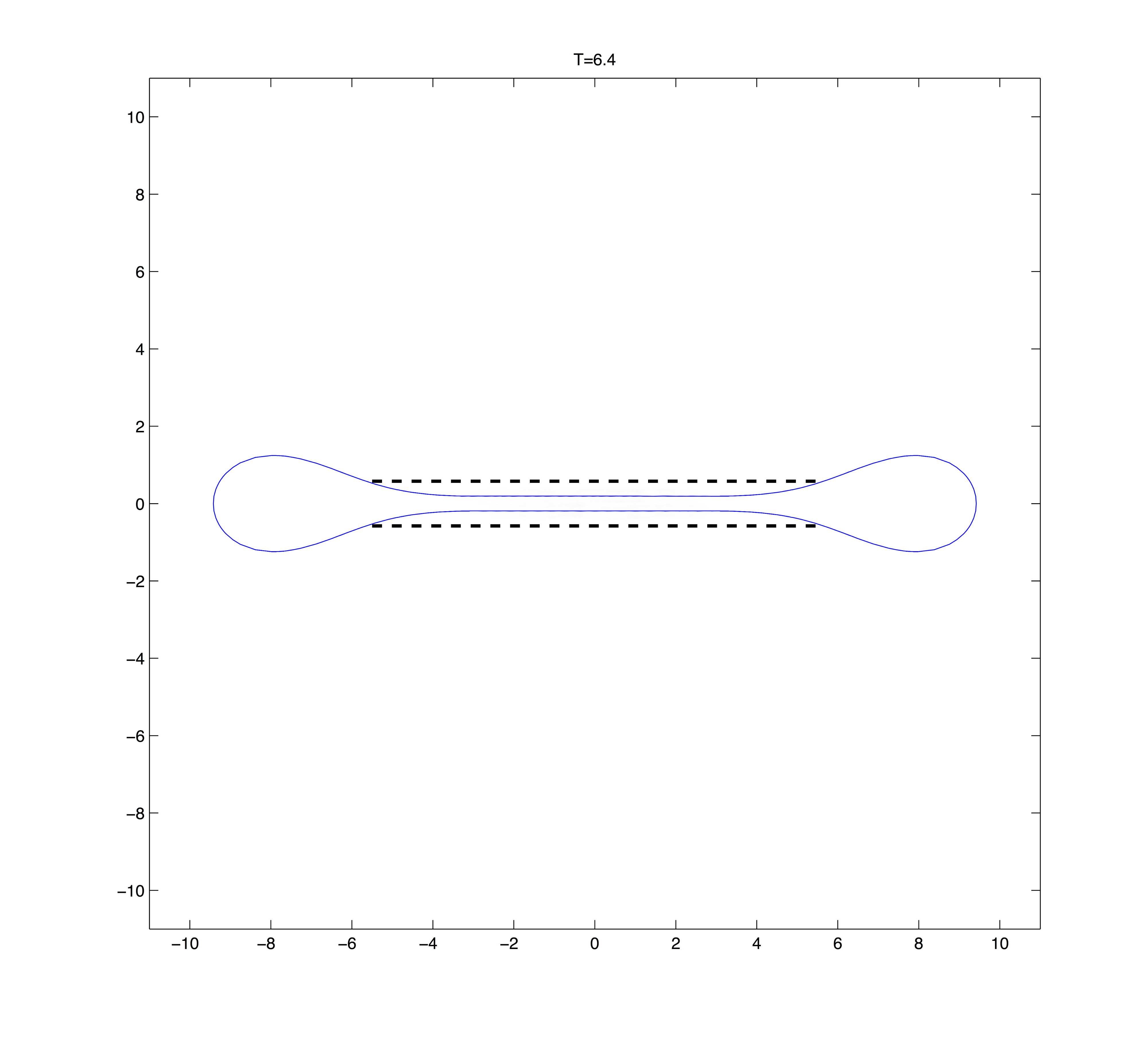 Figure 1
 Figure 2
 Figure 3
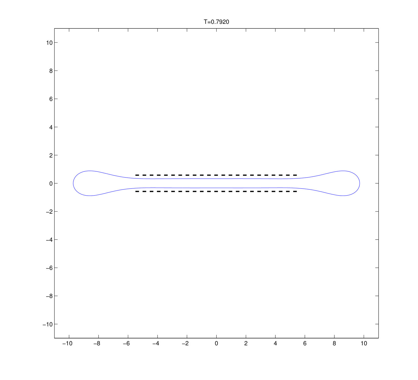 Figure 4
 Figure 5
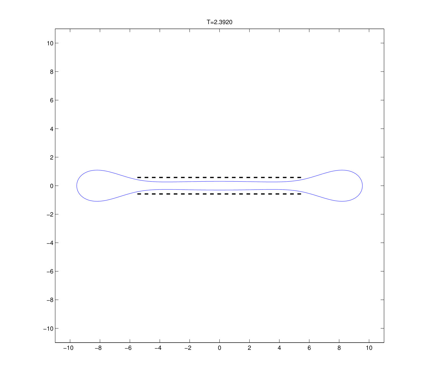 Figure 6
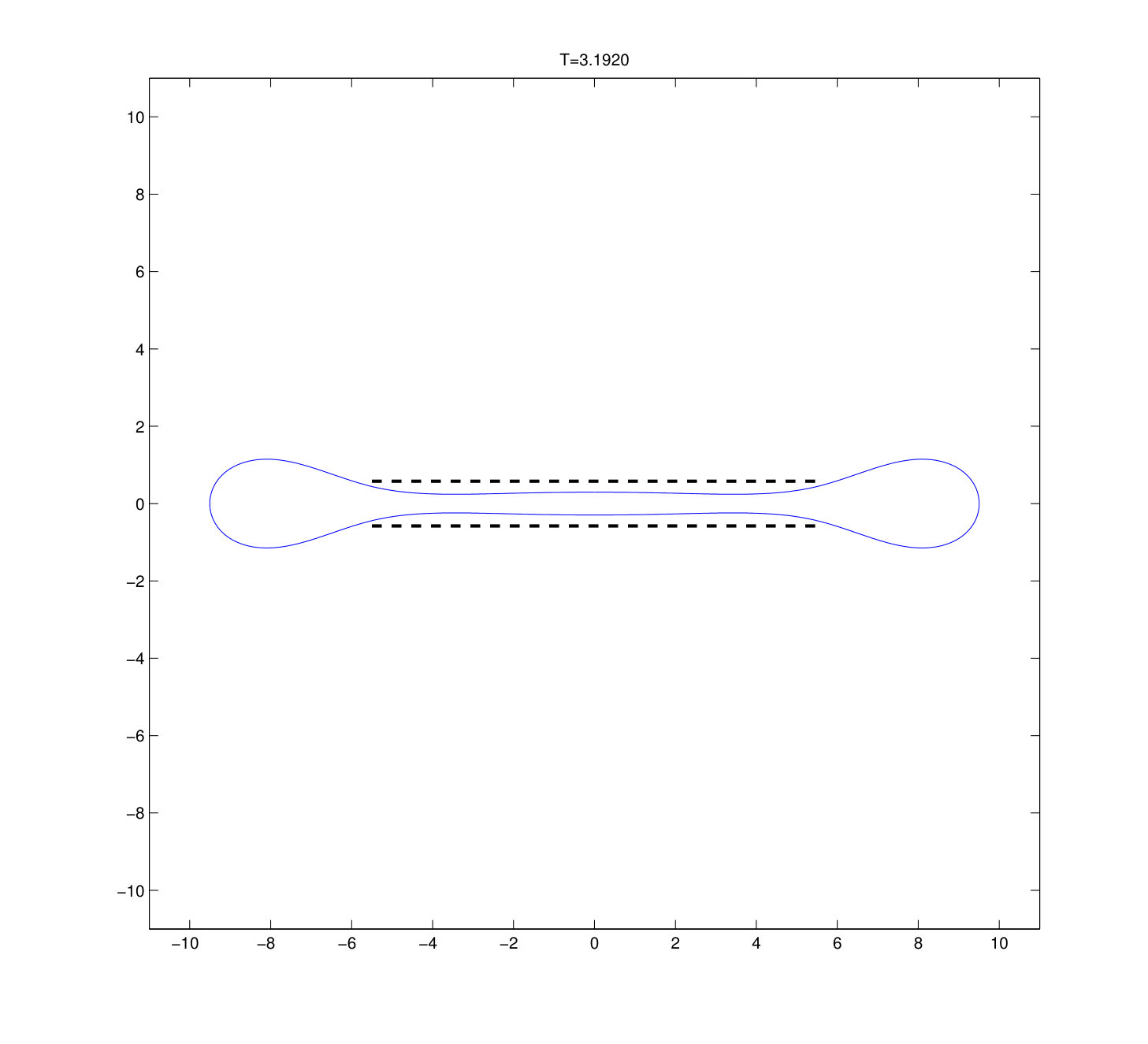 Figure 7
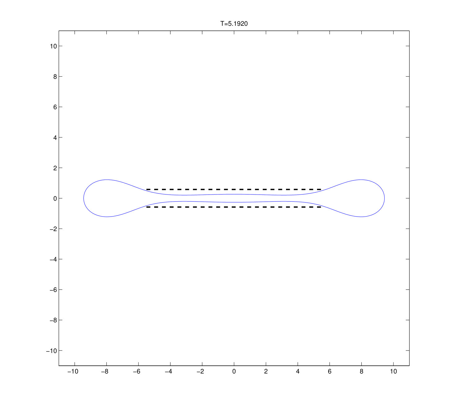 Figure 8
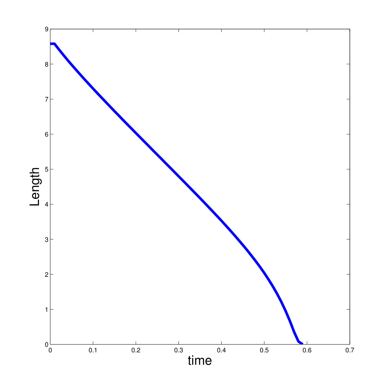 Figure 9
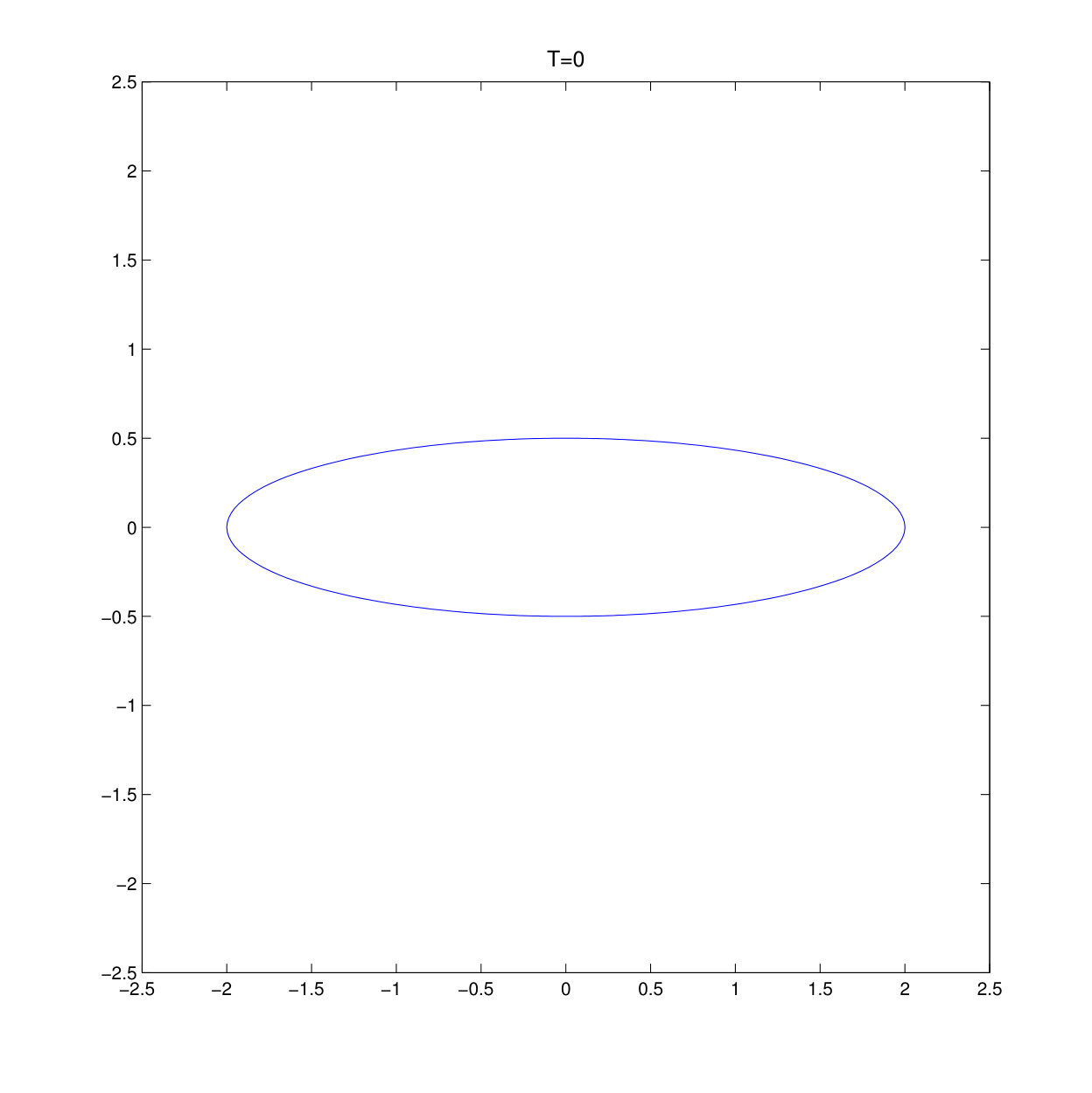 Figure 10
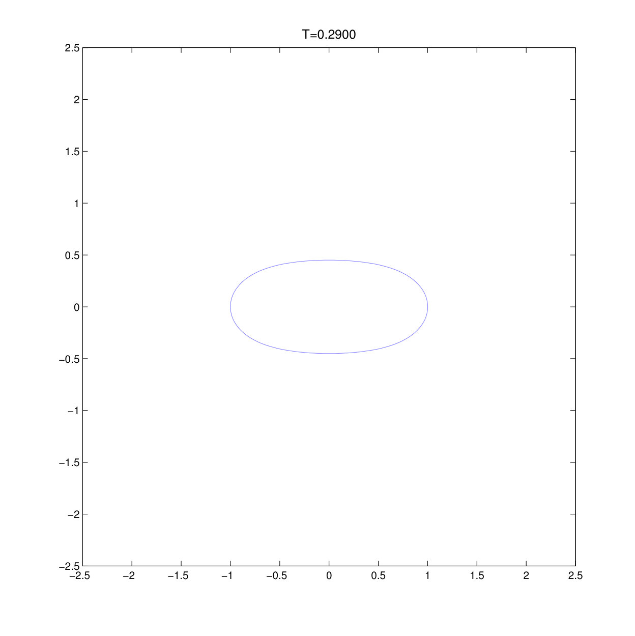 Figure 11
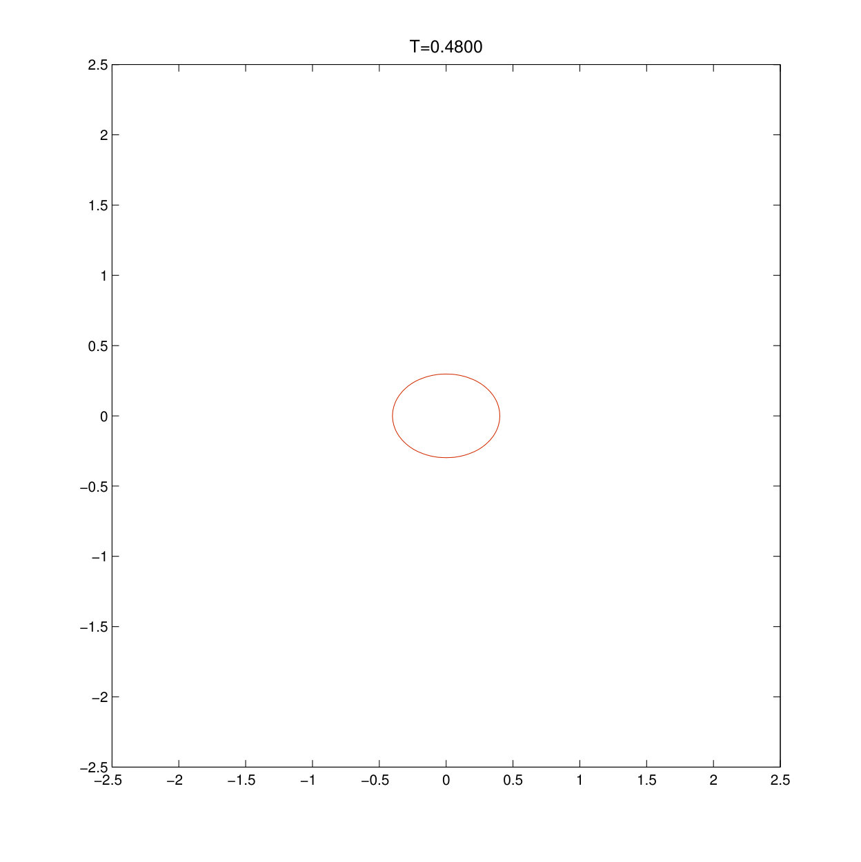 Figure 12
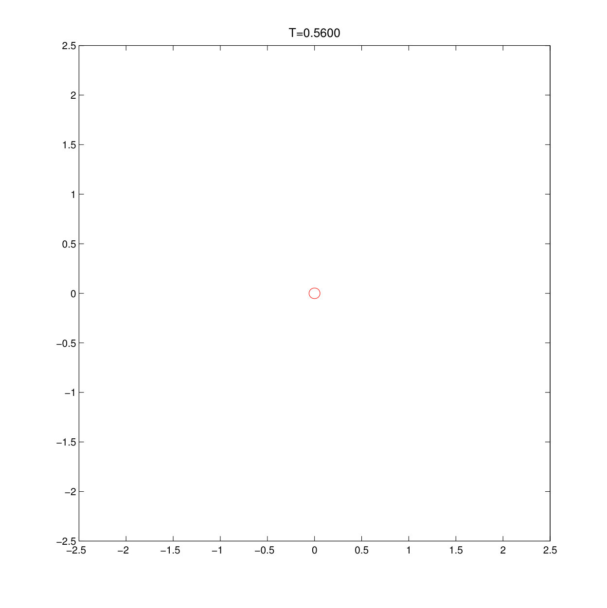 Figure 13
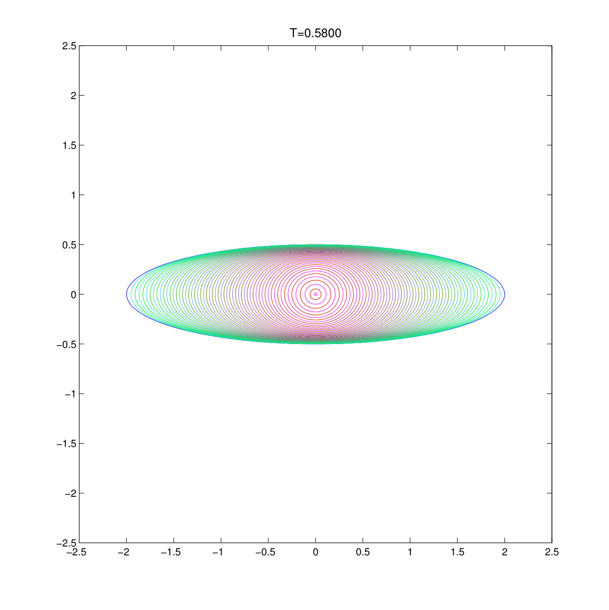 Figure 14
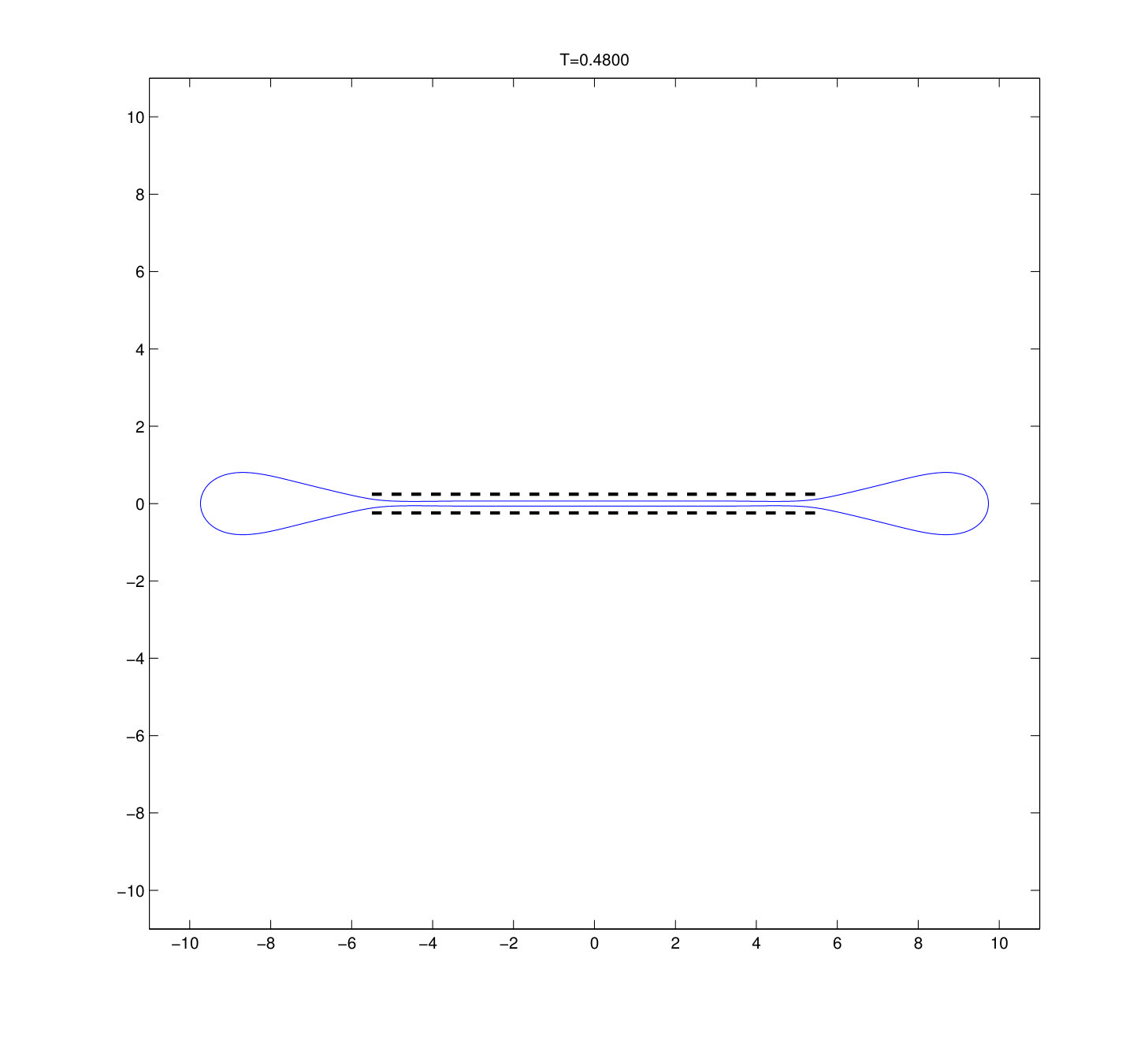 Figure 15
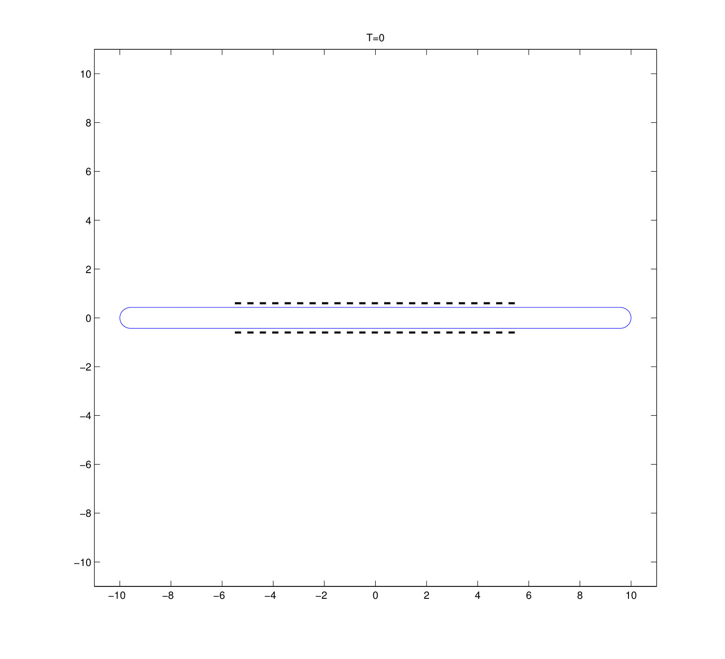 Figure 16
 Figure 17
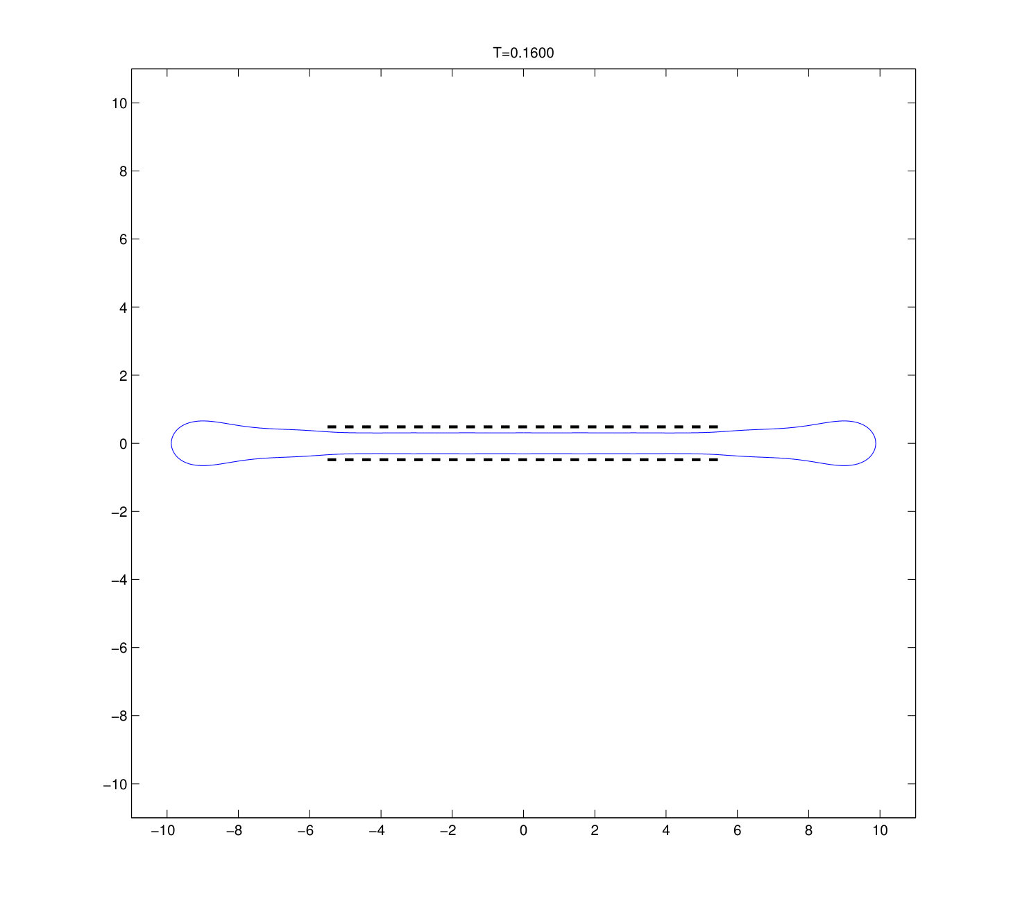 Figure 18
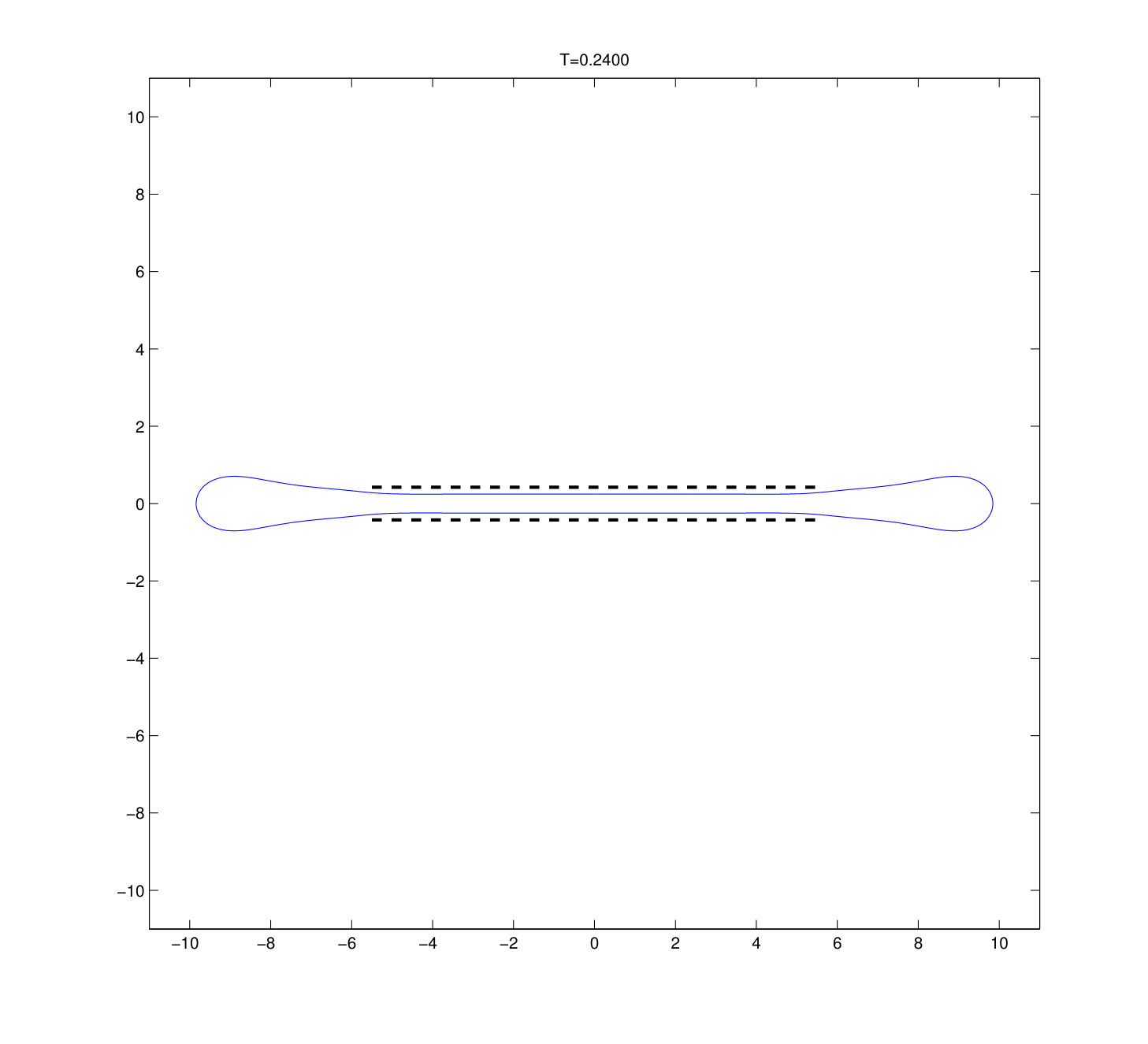 Figure 19
 Figure 20
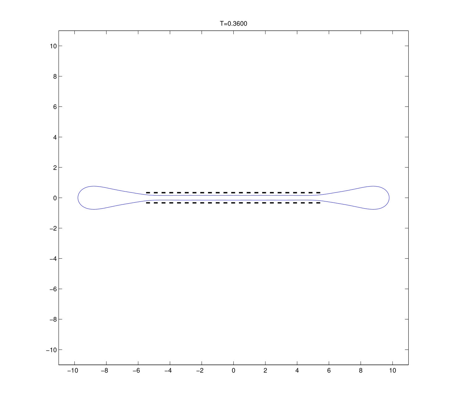 Figure 21
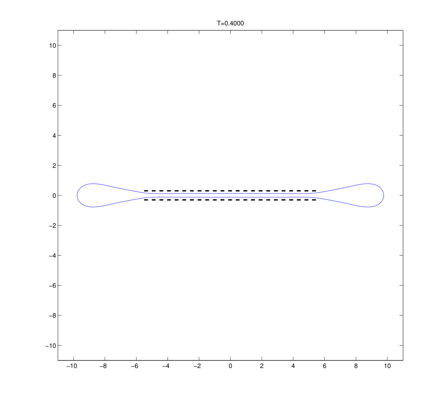 Figure 22
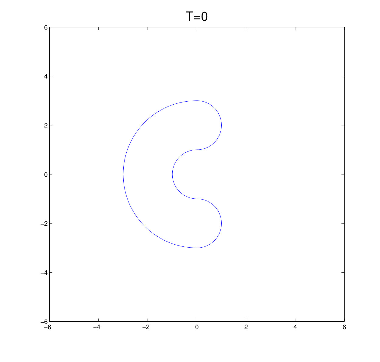 Figure 23
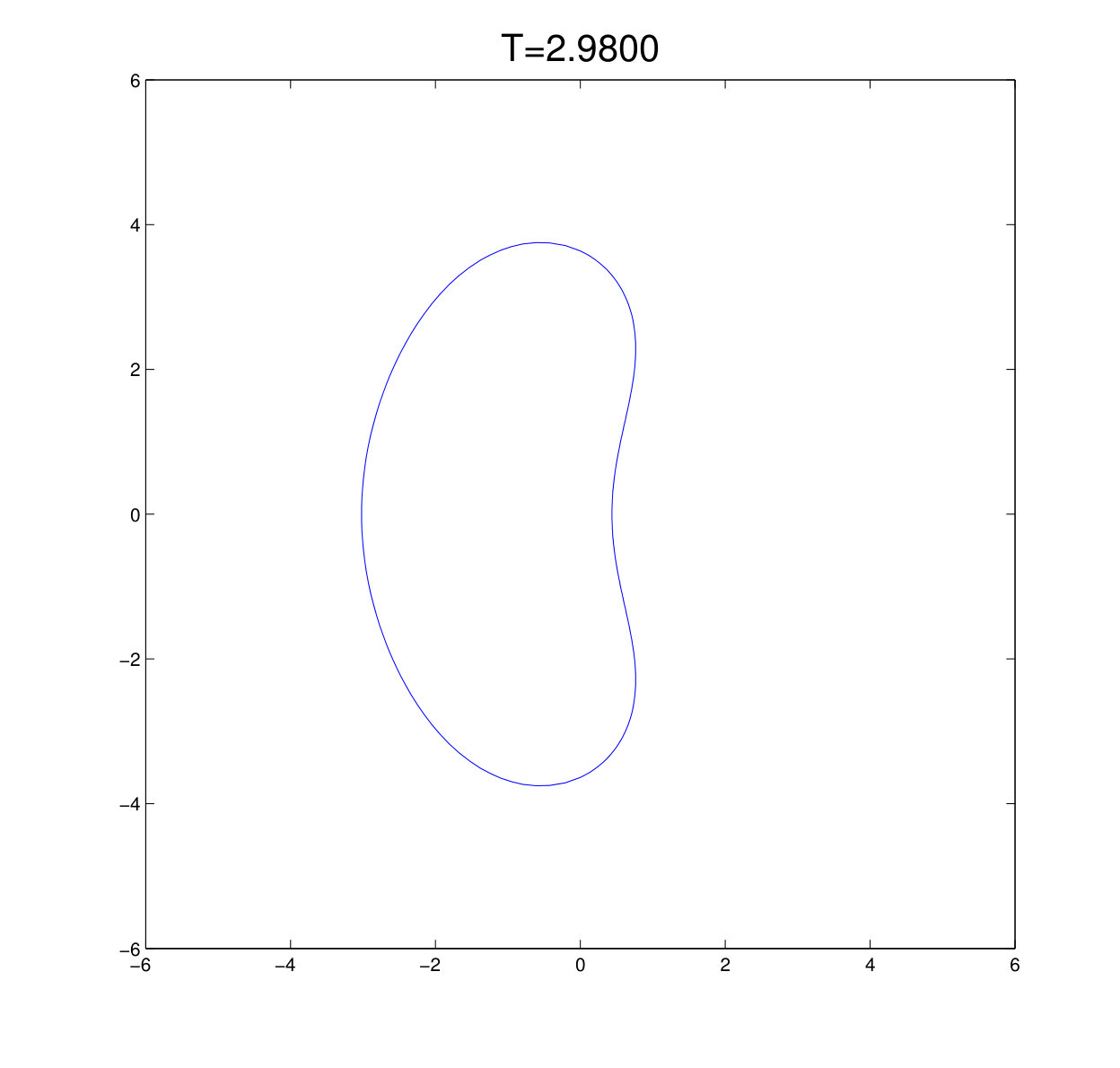 Figure 24
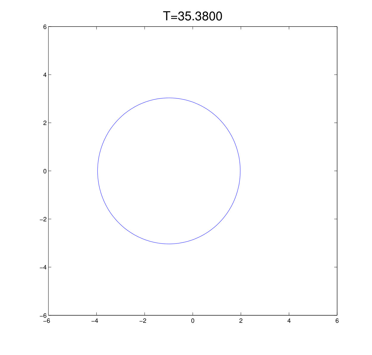 Figure 25
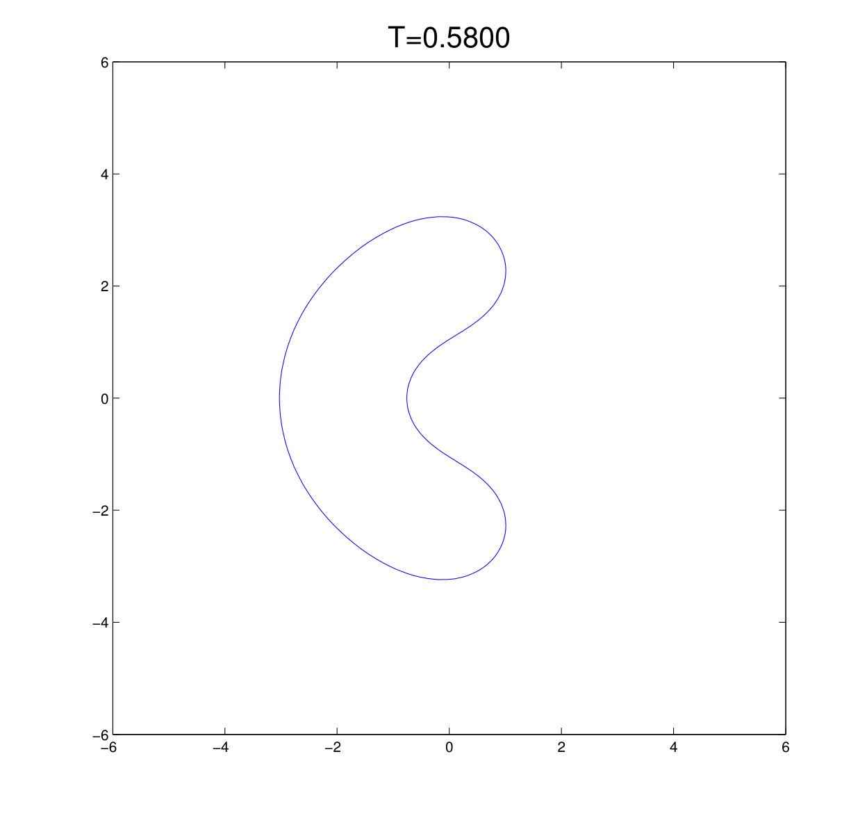 Figure 26
 Figure 27
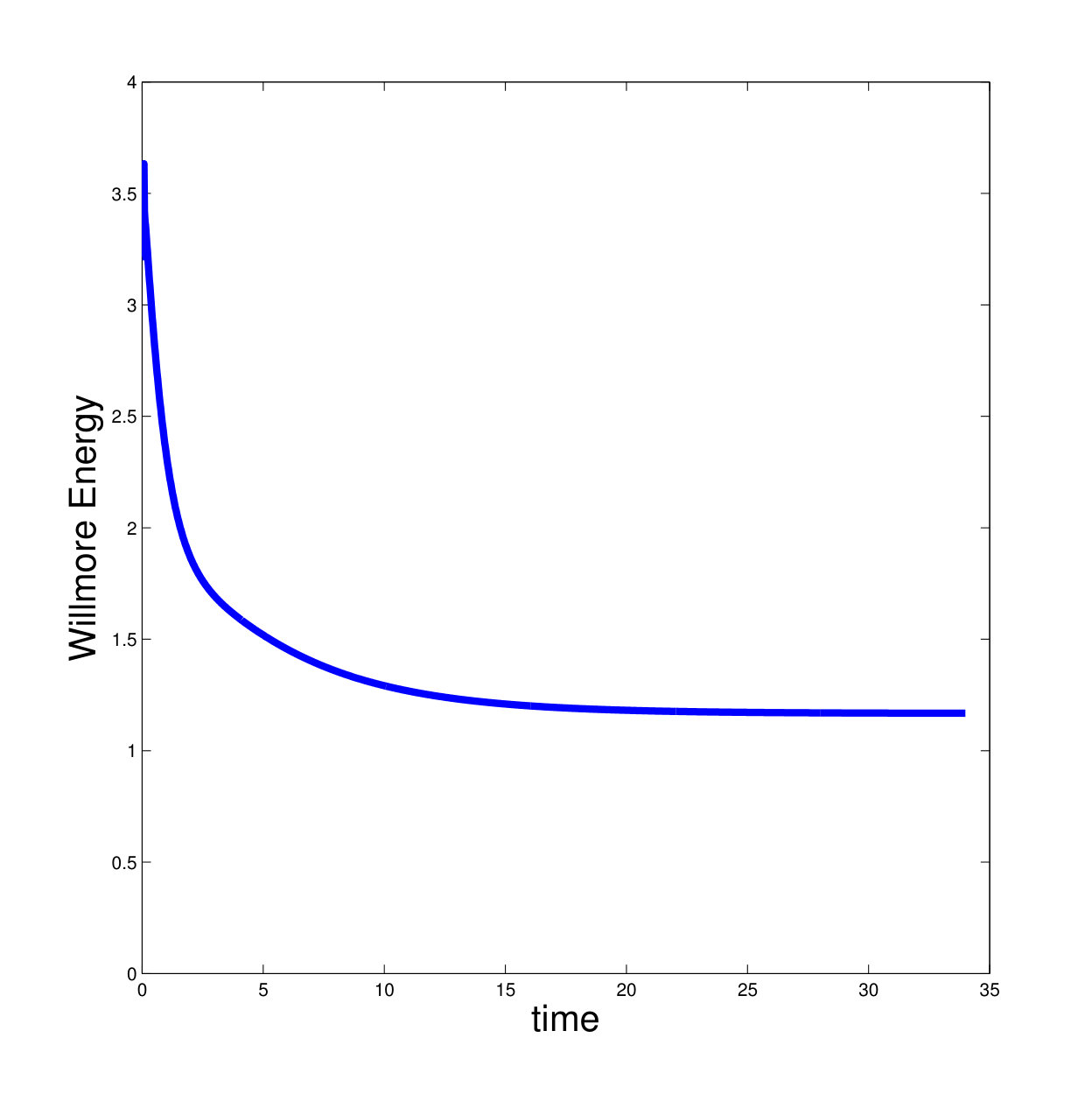 Figure 28
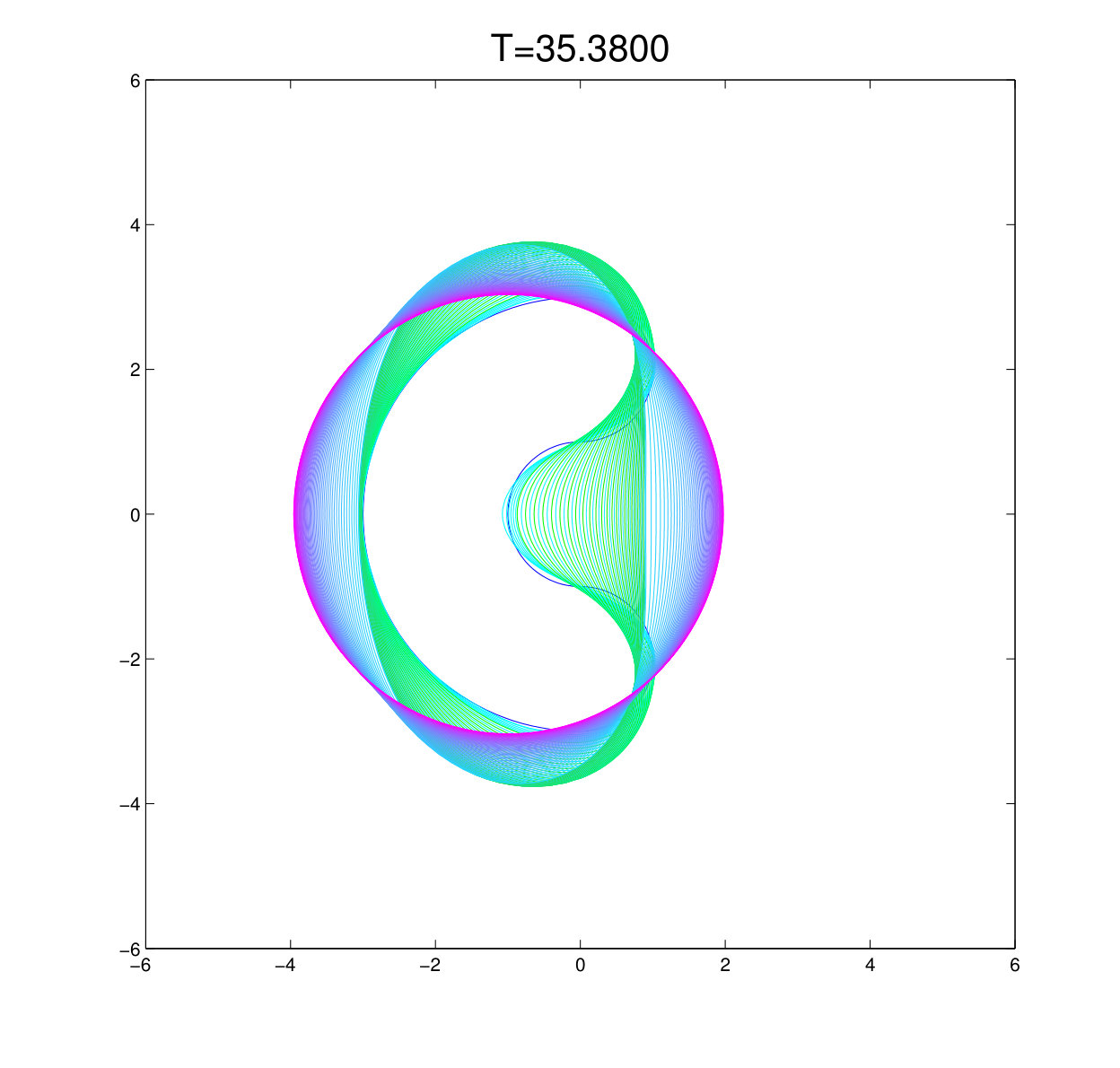 Figure 29
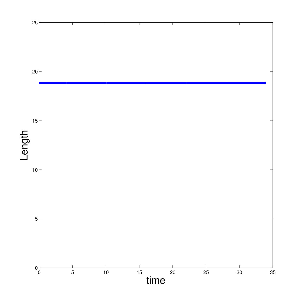 Figure 30
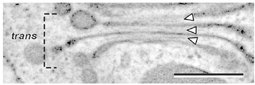 Figure 31
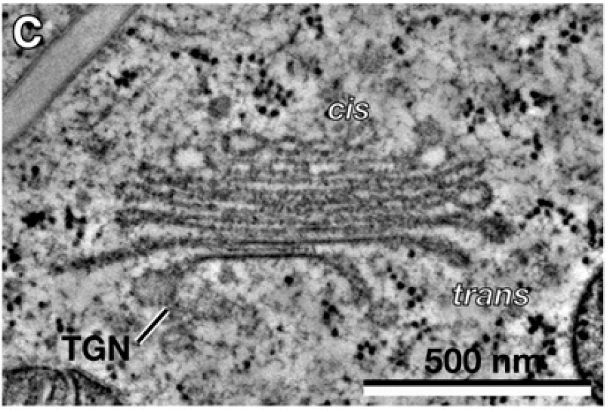 Figure 32
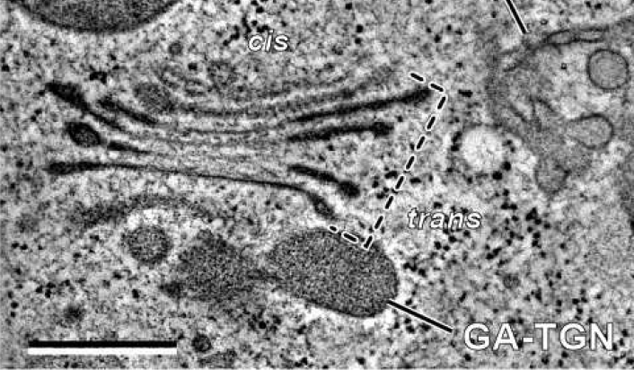 Figure 33
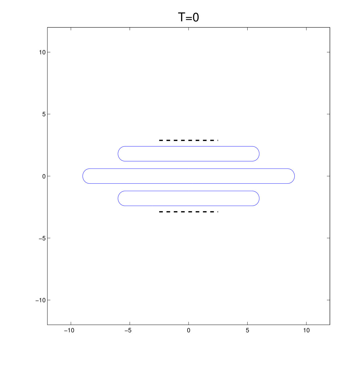 Figure 34
 Figure 35
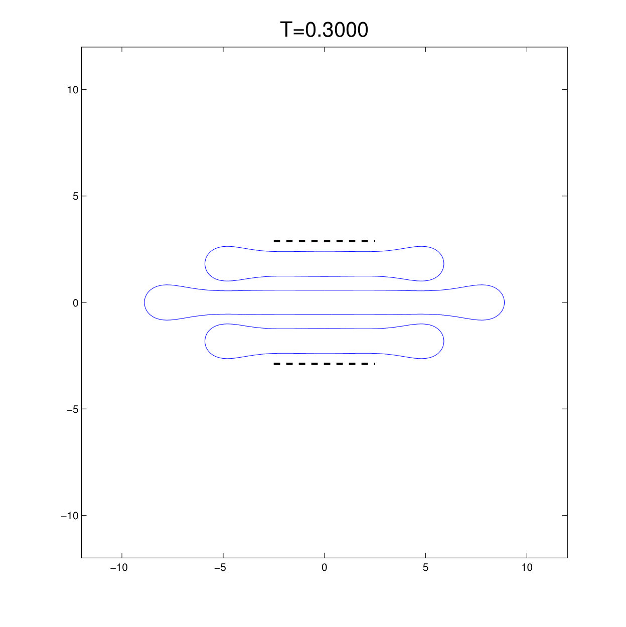 Figure 36
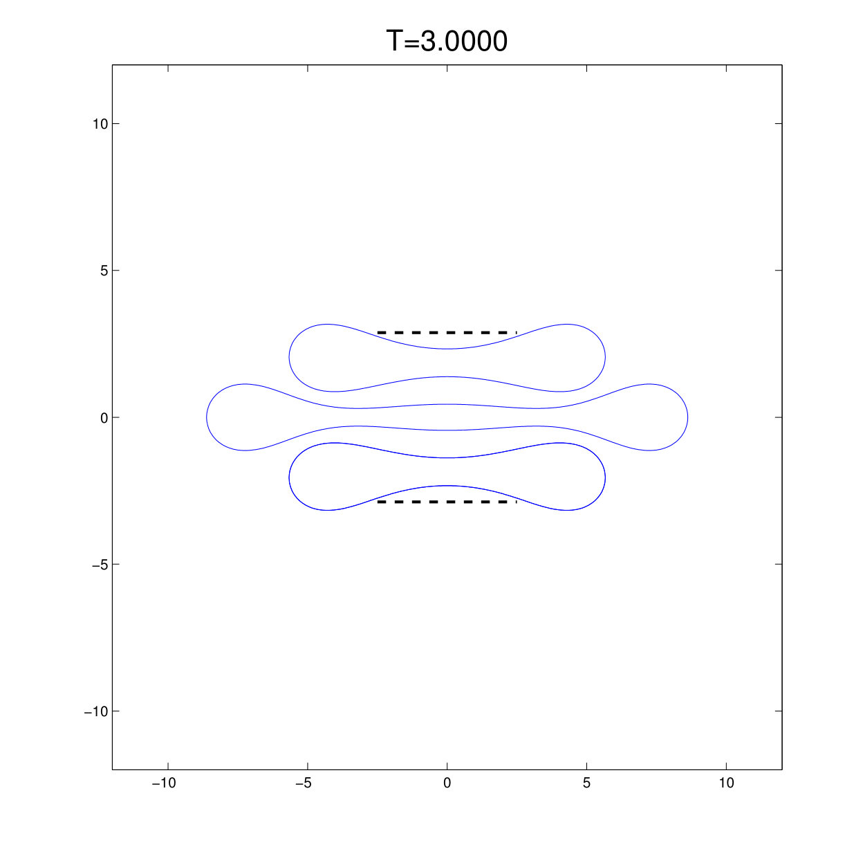 Figure 37
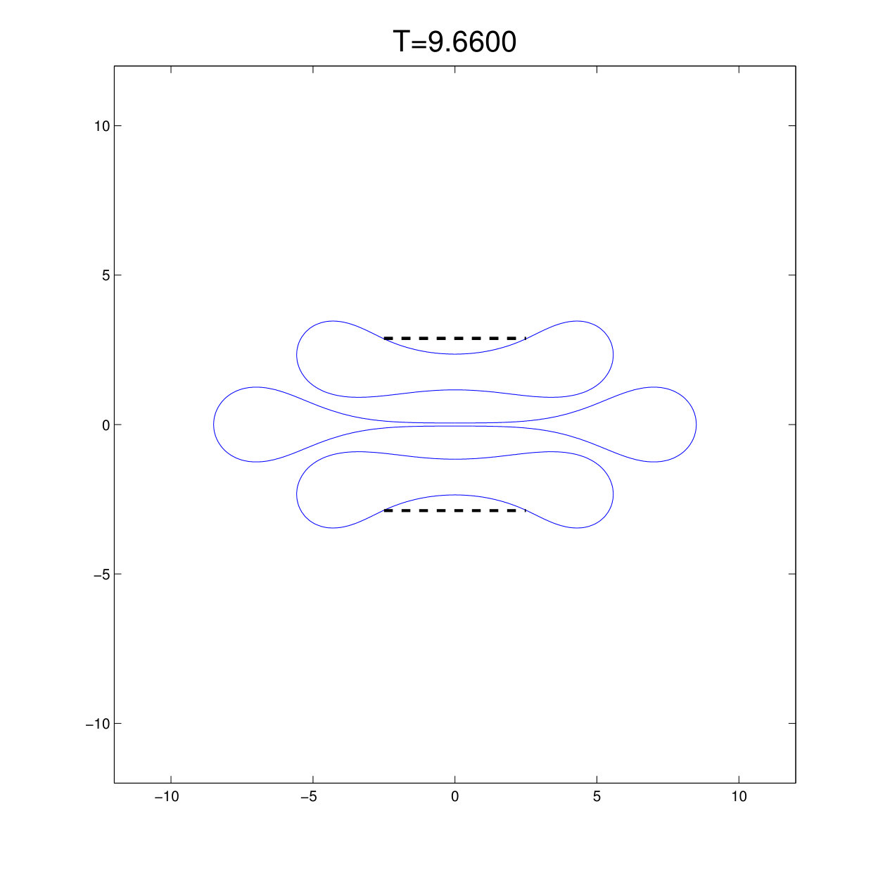 Figure 38
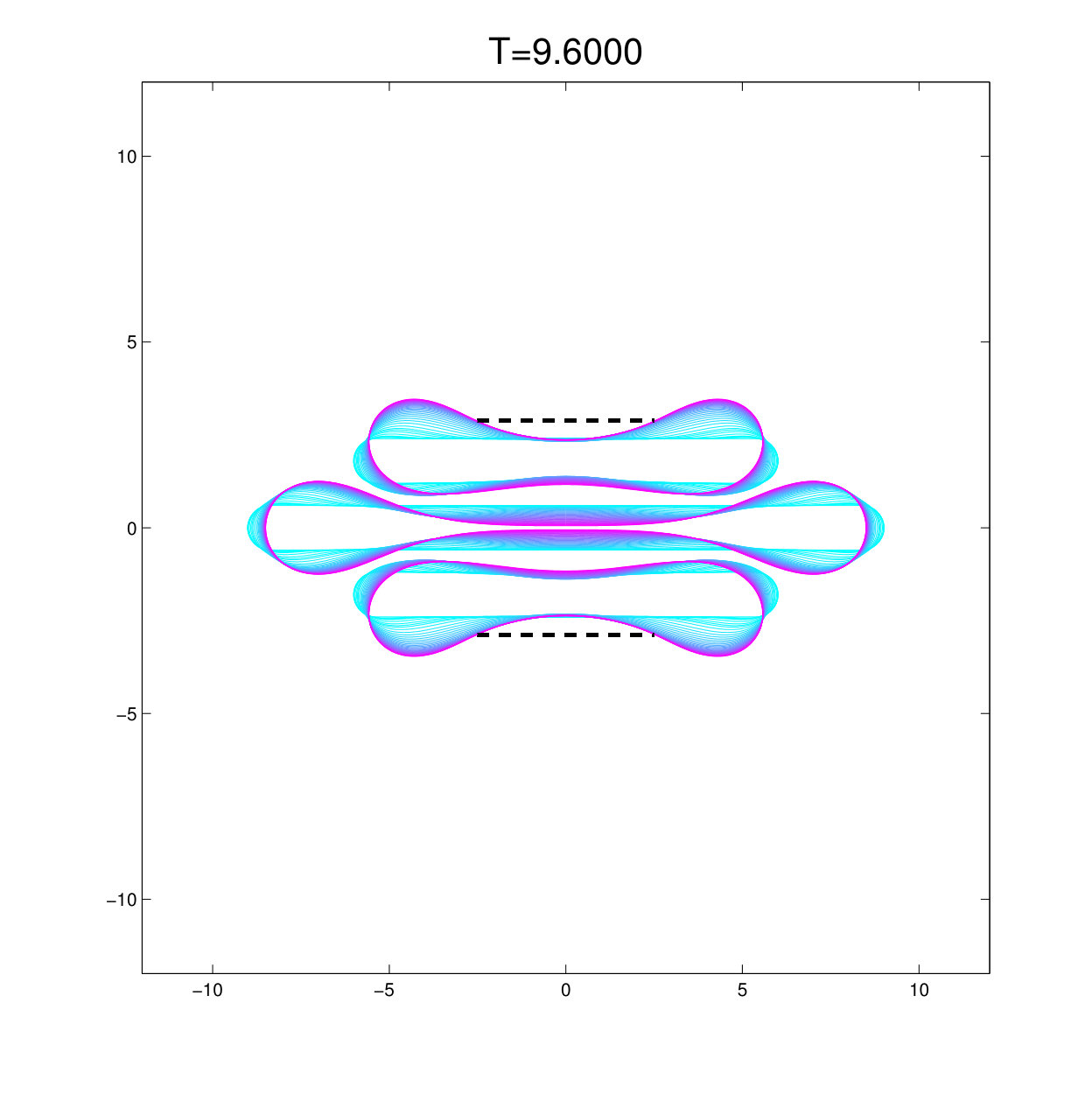 Figure 39
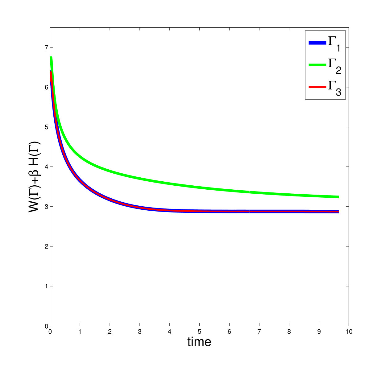 Figure 40
| FEM | Finite Element Method |
| SDG | Staggered Discontinuous Galerkin |
| the set of real numbers | |
| a hypersurface of dimension embedded in | |
| outer unit normal vector field | |
| Euclidean norm | |
| The space of polynomials of degree 2 defined over the set | |
| continuously differentiable functions | |
| tangential gradient of | |
| tangential Jacobian matrix of | |
| tangential divergence of | |
| tangential Laplace of |
Peer Reviews
No public reviews on file for this paper yet. If you reviewed it on a platform where reviews are public (OpenReview, ICLR, NeurIPS, ICML), you can paste yours below so the community can read it here.
Videos
No videos yet. Explain this paper in a talk, walkthrough, or lecture? Add one.
Taxonomy
TopicsCellular transport and secretion · Lipid Membrane Structure and Behavior · Advanced Fluorescence Microscopy Techniques
Parametric FEM for Shape Optimization applied to Golgi Stack
CHEN, Xinshi
A Thesis Submitted in Partial Fulfilment
of the Requirements for the Degree of
Master of Philosophy
in
Mathematics
The Chinese University of Hong Kong
July 2017
Thesis Assessment Committee
Professor CHAN Hon Fu Raymond (Chair)
Professor CHUNG Tsz Shun Eric (Thesis Supervisor)
Professor LUI Lok Ming (Committee Member)
Professor KIM Hyea Hyun (External Examiner)
Abstract
The thesis is about an application of the shape optimization to the morphological evolution of Golgi stack. Golgi stack consists of multiple layers of cisternae. It is an organelle in the biological cells. Inspired by the Helfrich Model [2], which is a model for vesicles typically applied to biological cells, a new model specially designed for Golgi stack is developed and then implemented using FEM in this thesis.
In the Golgi model, each cisternae of the Golgi stack is viewed as a closed vesicle without topological changes, and our model is adaptable to both single-vesicle case and multiple-vesicle case. The main idea of the math model is to minimize the elastic energy(bending energy) of the vesicles, with some constraints designed regarding to the biological properties of Golgi stack. With these constraints attached to the math model, we could extend this model to an obstacle-type problem. Hence, in the thesis, not only the simulations of Golgi stack are shown, some interesting examples without biological meanings are also demonstrated. Also, as multiple cisternaes are considered as a whole, this is also a model handling multiple objects.
A set of numerical examples is shown to compare with the observed shape of Golgi stack, so we can lay down some possible explanations to the morphological performance of trans-Golgi cisternae.
ACKNOWLEDGMENTS
I would like to express my sincere gratitude to Prof. Eric CHUNG, who took me as his M.Phil. student two years ago. It is with this chance he gave me that I could participate this awesome graduate program in Department of Mathematics in CUHK. His constant guidance on my thesis research through the past two years is of great importance to me. Besides, I wish to express my appreciation to Prof. Raymond CHAN, who provided me with many opportunities of presenting my work in some meetings and symposium. Here I extend my gratitude to Prof. LUI Lok Ming and Prof. KIM Hyea Hyun, for spending their precious time on the examination of my thesis research.
Besides, I want to thank all the faculties, staffs and colleagues that I met in CUHK Math Department, for their various kinds of supports to my two years’ study. Especially, I want to thank my group-mates including Dota Chi Yeung LAM, Tony Siu Wun CHEUNG, Nina Yue QIAN, Ivan Tak Shing AU YEUNG, Simon Sai Mang PUN, John Ming Fai LAM, Tommy Chor Hung LI, and quasi-group-mate John Yufei ZHANG, who give me countless help and bring me lots of fun everyday.
Last but not least, I would like to delicate this thesis to my parents, Mr. and Mrs. CHEN, and my boyfriend, Rui, for their unconditional company and support.
Contents
Abbreviations and Notations
Chapter 1 Introduction
The thesis project is a mathematical modeling on the shape evolution of Golgi stack. This project was proposed by Prof. Kang from Life Science Department, and the final goal of this project is to mimic the growing process of Golgi stack so as to give a potential explanation to some special properties of the observed shapes of Golgi stack mathematically. The following image is shown to give a first impression of the Golgi stack [1].
A Golgi stack consists of multiple layers. Each layer is a Golgi cisternae. The cisternae in different stages has different morphological performances. Those stages are called cis-, med- and trans-. For the cis-Golgi, the cisternal assembly is in process, but in the trans-Golgi, the assembly is finished. Our model mainly concerns with trans-Golgi cisternae, for which we can view each layer(cisternae) as a vesicle with closed surface without topological changes.
Our math model is constructed by forming a series of geometric evolution equations. Suppose is the surface of a vesicle, which represents one Golgi cisternae. There are four shape functionals considered in our model defined on . First, the Willmore energy , where is the mean curvature. It is believed that the shapes of the biomembranes are closely relevant to the elastic energy. Because Willmore energy is equivalent to the elastic energy under certain condition, which is explained in Section 1.1.1, we regard the Willmore energy as the dominant energy in our model of Golgi stack. Second, the area functional . The model include this functional to serve for the surface area constraint. Because the number of molecules is believed to be fixed in our model, the surface area of the shape is conserved. Third, a heaviside functional , where is an indicator function. To mimic the barriers (the intercisternal elements for Golgi stack) above and belong each Golgi layer, we form this new functional by integrating the heaviside function. Note that the set represents the region of the barriers/obstacles. Fourth, a distance functional . When multiple vesicles are considered as a whole, the intersection of them should be avoided. Hence, this distance functional is included to handle the relations among those objects. We couple these functionals to form the model. Then we implement it by parametric finite element method, using Matlab.
The followings are the main results of the Golgi simulation. First, for a single layer of trans-cisternae, we mimic the evolution process of the cisternae when the protein vesicles bud from the marginal part of the cisternae. The numerical result explains that it is the barriers placed above and below the cisternae that inhibit the vertical expansion of the cisterae. Second, it is revealed from our result that the swelling of the marginal regions of the trans-cisternae thins its central part to decrease the elastic energy. Third, we also mimic the shape evolution of Golgi with multiple cisternae stacked upon each other. All these simulations are done by mathematical computation, which may give a potential explanation to the mechanism of the Golgi stack.
What’s more, the model can also be extended to more general cases without biological meanings. In Section 5.1, many examples of the applications of this model are demonstrated.
1.1 Overall Introduction and Motivation
In this section, I describe the construction of the math models with explanations on the corresponding biological properties of Golgi stack. From now on, we use the geometric surface to describe the surface of a single Golgi cisternae, which is assumed to be a closed vesicle without topological changes. For the case including multiple layers of Golgi cisternaes in one model, we use the family , where each layer of Golgi cisternae is represented by a surface for some . The followings are four important functionals related to the thesis.
1.1.1 Willmore Energy
First, based on a well-accepted fact suggested in some previous works [2, 3, 4, 5, 6] that the biomembranes are closely related to elastic energy, we consider the elastic energy as the dominated energy to be minimized in our model. We include this energy because is also a surface of biomembranes. The elastic energy, also named bending energy, to the lowest order, take the form
[TABLE]
where the integral is taken over the surface , is the bending rigidity with respect to mean curvature and is the bending rigidity with respect to Gaussian curvature. and are the mean and Gaussian curvature respectively defined as . and are the principle curvatures. Assume that is a closed surface. Gauss-Bonnet Theorem [7, Ch. 8] tells,
[TABLE]
where is the Euler characteristic of , which is topological invariant. Hence, we only need to consider the Willmore energy [8]
[TABLE]
when is a closed surface without topological changes. In summary, to find the optimal shape of Golgi cisternae by minimizing the Willmore energy is the first main point in our model.
1.1.2 Area Constraint
Second, in many cell models, the surface area of a cell is set to be fixed [2, 3]. Agreed by Prof. Kang (Life Science Department), we assume the surface area of each trans-Golgi cisternae is conserved. This is based on the fact that the cisternal assembly is completed for tran-cisternae, so the number of molecules of the membrane surface is assumed to be invariant. To enforce this constraint, we consider the functional defined by
[TABLE]
which indicates the area of the surface . Utilizing this functional, we impose the area constraint into the model.
1.1.3 Barrier Functional
Third, we want to include the inter-cisternal elements of Golgi stack, which is biologically relevant to the membrane stacking, into our model. The inter-cisternal elements may limit the expansion of Golgi cisternae in the lateral direction. It serves as the obstacles/barriers placed above and below each Golgi cisternae. To model these restraining factors, we construct a shape functional by the integration of an indicator function , where is a subset of indicating the region of the obstacles. We define the functional as
[TABLE]
where is the identity on . We want to include this functional to our model so that the surface gets hard to cross the region indicated by the set . Detailed explanation of the usage of this functional is given in Section 3.2.
1.1.4 Distance Functional - for multiple vesicles case
Fourth, Golgi stack consists of multiple layers of Golgi cisternaes. When multiple vesicles are placed in one model, the interaction among the vesicles should be considered. In other words, the vesicles should not cross each other, and even the repulsion between the vesicles should be taken into consideration, because the lipid bilayer structure of the bio-membranes could cause repulsion when the vesicles approach each other. In this case, we consider the distance among the cisternaes. We also use it to construct a functional . The detailed formulas and explanations are demonstrated in Section 3.3. In summary, is built to control the multiple vesicles case.
1.2 Outline
- •
Chapter 2: The preliminary definitions and lemmas related to the thesis are stated. Most of them are in the field of Differential Geometry. Though we did not work on the theories of Geometry, the theoretical results worked by the predecessors are important for us to construct the numerical algorithm.
- •
Chapter 3: The detailed constructions of three models are illustrated. Model 2 and Model 3 are main contributions of this thesis. The three models are introduced in Section 3.1, 3.2 and 3.3 respectively. In each of the section, the motivation of building the model, the idea of the model and the detailed problem setting of the model are stated.
- •
Chapter 4: In the first part of this chapter, the detailed explanation of the time discretization and the space discretization (the construction of the mesh) is given. In the second part, the linearization of some nonlinear functions are illustrated, and then the fully discretized weak formulas for the discrete problems are written for each model introduced in Chapter 3. Finally, the full algorithm is given.
- •
Chapter 5: The first part of this section gives some numerical examples without biological meanings, only to demonstrate the models and to see the conservation of and the decrease of the energy. The second part gives some simulations of Golgi stack, including single cisternae case and multi-cisternae case. Some possible explanations to the morphological properties of the Golgi are given, according to the comparison of the numerical results and the observed Golgi.
1.3 Previous Work and Our Contributions
The mathematical study of the shape of biomembranes is introduced by the Helfrich model in 1970s [2, 3], which is a model aiming to study the equilibrium shape of vesicles dominated by elastic energy (or called bending energy). After that, further works on this topic have been done [5, 6, 9, 11, 10, 12, 13, 14, 15], including theoretical analysis and numerical implementation. Many of them applied FEM [11, 10]. Besides, other methods were also studied, for instance, finite difference method [13], level set method [14] and discrete Willmore flow method [15]. Previous works give us inspirations. For example, the Lagrange Multiplier Method is commonly used for the area constraint. Also, previous studies provided excellent formulas for the shape derivative of Willmore energy.
In the thesis, I introduce three models in Section 3.1, 3.2 and 3.3 respectively, and then these models are implemented by FEM with the algorithm stated in Chapter 4. In Section 3.1, it brings out a model dominated by the Willmore energy with conservation of the surface area. This is not a new model developed and solved by us. The works mentioned above [9, 11, 10, 12] have studied this model. Some of them only includes the area constraint [9, 11]. Some also take the volume into account [10, 12]. If one includes both the area and volume constraints, the numerical results could explain the concave shape of the blood cells in a numerical way [2, 10].
Besides, Model 2 (Section 3.2) and Model 3 (Section 3.3) are presented in Chapter 3. These two models are constructed by considering the properties of the Golgi stack and these are the main contribution of our work. Model 2 is an extension of Model 1 by adding some obstacles into the problem. This is inspired by the existence of some biological elements which locate above and below each Golgi cisternae and may confine the vertical extension of the cisternae. Besides, as those confining elements could be moving, we also demonstrate the examples of the moving obstacles. Model 3 is designed for the Golgi stack of multiple cisternaes as a whole. These cisternaes could not cross each other, and even the repulsion of their surface should also be considered. Hence, our method could handle the problem with multiple objects. In summary, Model 2 and 3 are newly formed by us, and we also implement the models by FEM. The numerical results are shown in Chapter 5.
Lastly, by comparing our numerical simulation of the Golgi trans-cisternae to the observed Golgi, some possible explanations are drawn on the morphological performance of the trans-cisternae.
Chapter 2 Mathematical Background
The theoretical background of this research is introduced in this chapter. It contains many theories in the field of Differential Geometry. Without the theoretical results of Geometry worked by the predecessors, the numerical methods will be hard to implement. In this chapter, denotes a hyperspace embedded in , which is piecewise smooth. The mathematical concepts and theories defined on , which are relevant to this thesis research, are presented.
2.1 Tangential Calculus
Definition 2.1.1**.**
**(Tangential Gradient)
**The tangential gradient of a function is defined as
[TABLE]
where is a smooth extension to such that .
Remark 2.1.2*.*
The value of is independent on the extension function chosen.
With the above definition, we can write down the corresponding tangential Jacobian matrix for a vector function :
[TABLE]
Definition 2.1.3**.**
**(Tangential Divergence)
**The tangential divergence of a function is defined as
[TABLE]
where represents the trace of the matrix.
Definition 2.1.4**.**
**(Tangential Laplace-Beltrami operator)
**The tangential Laplace of a function is defined as
[TABLE]
2.2 Shape Differential Calculus
Consider a domain and a functional defined on in the following form
[TABLE]
Consider a family of transformations of , . Denote the transformation by such that and . We assume that is a diffeomorphism from to (see [17, Ch. 5] for the definition of diffeomorphism). Denote by the domain containing for all . Let be the velocity field associated with the transformation , then we can arrive at the following definition.
Definition 2.2.1**.**
(shape derivative) Suppose is shape differentiable at (see [17, Ch. 5] for the definition). The shape derivative at according to the direction is defined as
[TABLE]
where the transformation is associated with .
Here are two examples of the formulas of shape derivatives of the functional , where is the mean curvature. And the detailed derivations of these formulas are provided in [10] and [11]. Note that .
[TABLE]
[TABLE]
where .
Recall the functional
[TABLE]
Now suppose the function value of only depends on . In other words, the function value can be represented by . According to [18, Ch. 2], the following lemma is applicable.
Lemma 2.2.2**.**
Suppose is independent on the geometry and is of class . Then in the direction ,
[TABLE]
For example, this lemma can be applied to the functional . Here is clearly independent of . One can simply apply Lemma 2.1.6 to obtain the formula
[TABLE]
Since (see [19]), where represents the conormal vector, and the surface we consider do not have boundary. Hence, we arrive at the following equation that we widely use in our work:
[TABLE]
Chapter 3 Model and Problem Setting
3.1 Willmore energy with Area Constraint
With the functionals introduced above, we can define a functional dependent on the specific problem we are working on, and this functional functions as the dominant energy that we want to minimize on the surface . To track the motion of dominated by the energy , a typical way is to define a geometric evolution equation using the shape derivative . Hence, the main idea of our numerical method to solve the shape evolution is to find the velocity , which satisfies the equation
[TABLE]
where is a Hilbert space of functions defined on .
Consequently, we can define different models by constructing different energies . In the following sections, I formula three sets of problems corresponding to three models, which can be numerically solved by the discrete schemes described in Chapter 4. In the following three sub-sections, each model is illustrated with detailed equations.
3.1.1 The Model 1 and the Functional
The model 1 is a basic model. It considers only one vesicle . The main idea of Model 1 is to minimize the Willmore energy under the condition that the surface area of is fixed. Hence, it does with the functionals and . They are briefly discussed in Section 2.1.1 and Section 2.1.2. The biological reason of the conservation of the area is also given in Section 2.1.2.
[TABLE]
where is a given initial shape. The confinement is imposed to the problem by using a multiplier . Then is formulated as
[TABLE]
We aim to find the optimal and .
3.1.2 Problem Setting of Model 1
First, we define
[TABLE]
and by
[TABLE]
for all and . Hence, we can regard . The goal is now to minimize the functional . Hence, it is a typical way to form an evolution equation in the form of (3.1). Consequently, we have the following problem setting.
Problem 3.1.1**.**
**(Willmore Flow with Area Constraint, Weak Form)
**For a given initial shape , find the multiplier and the function according to the family of surface , such that on the time interval ,
[TABLE]
[TABLE]
for all test function . The function space of will be later discussed.
The shape derivatives of the above functionals can be computed using the following equations
[TABLE]
or
[TABLE]
and
[TABLE]
The details of the first two equations can be found in [10] and [11]. The third equation is simpler, so its derivation is given in the Preliminary Section.
Some of the notations used in the above equations are explained as follows:
- •
is the vector form of mean curvature on the direction of the outer unit normal vector .
- •
is the identity on .
- •
is a symmetric tensor defined by .
The equation (3.7) and (3.9) are implemented for the Model 1.
This Model 1 is not a model firstly produced and solved by us. Instead, many works [9, 11, 10, 12] have been done on the study of this model, of which many also consider the volume constraint [10, 12]. In summary, Model 1 is a fundamental model, which has been studied for many years. However, it catches an important property of the bio-membranes, that the membranes is closely relevant to the elastic energy. Also, it imposes the idea that the number of molecules of the membranes is fixed such that the surface area of the membrane is conserved. If one includes one more constraint, the volume constraint, to Model 1, the numerical results can explain the concave shape of the blood cells mathematically [2, 10]. However, since our work is triggered by the shape evolution of Golgi stack, instead of considering the volume constraints, we consider other special properties of the Golgi stack and build our own models. The coming two sections present two models of Golgi stacks. Model 2 is designed for a singer layer of Golgi cisternae and Model 3 is designed for the Golgi stack of multiple cisternaes as a whole.
3.2 Willmore Energy with Area Constraint and Obstacles
3.2.1 The Model 2 and the Functional
Model 2 is an extension to Model 1 by considering the existence of some obstacles/barriers in the problem. This is motivated by a property of Golgi cisternae, which may be confined by the intercisternal elements above and below each Golgi cisternae layer. (See Section 2.1.3). In Model 2, the obstacles are considered and estimated by the functional
[TABLE]
defined in Section 2.1.3, where represents the region of the obstacles/barriers. One can easily observe that will take nonzero values only if . Hence, if we add this functional to the energy that we want to minimize, it will be hard for the shape to touch and cross the region so as to avoid the increase of the total amount of the energy.
To conclude, in Model 2, we want to do the same optimization as in Model 1, but also to include some obstacles indicated by the set . Normally, this model can be explained by the following problem:
[TABLE]
The resulted functional can then be formulated as
[TABLE]
which is the augmented energy to be minimized in Model 2.
Remark 3.2.1*.*
The constant is a weight of the functional to control the impact of . The dominated energy of our model should be the Willmore energy . is only a constraint. Hence, we don’t want the functional to dominate the whole energy .
3.2.2 Problem Setting of Model 2
Use the same notation as those in Section 3.1.2, we can form the following weak problem to minimize .
Problem 3.2.1**.**
**(Willmore Flow with Area Constraint and Obstacles, Weak Form)
**Suppose that is fixed as a weight coefficient. Now given , find and the function such that on the time interval ,
[TABLE]
[TABLE]
for all test function .
The calculation of is discussed as follows.
Since the indicator function is discontinuous, the implementation of it using FEM is not applicable. In the finite element method, we choose a smooth version of the indicator. More precisely, assume that represents a very regular shape. Then, can be written as a composition of the heaviside function
[TABLE]
Remark 3.2.2*.*
For example, if , then it can be written as a composition of by
[TABLE]
Though is still a discontinuous step function, we use the smooth approximation
[TABLE]
of it. Now a smooth version of is obtained.
With the smoothness of , we can now derive the formula for . By lemma 2.2.2, the formula of is obtained:
[TABLE]
Remark 3.2.3*.*
Usually, in the math models, is some fixed obstacles and independent of time. However, inspired by the hypothesis mentioned by Prof. Kang, that the intercisternal elements (such as Golgi matrix, which works as the constraining factor in our math model on Golgi stacks) maintain the same distance with the membrane since some of its components are embedded in the membrane. Hence, it could be more realistic to keep the distance between the membrane and the barriers when we mimic the growing process of Golgi cisternae. Nevertheless, since the shape of the cisternae evolves with time, the position of the barriers also need changesx to keep the distance. Based on this, we also make some numerical experiments for the moving obstacles . These examples can be found in Chapter 5.
3.3 Multiple Vesicles Case
3.3.1 The Distance Functional
As succinctly introduced in Section 2.1.4, the Golgi stack consist of multiple layers of Golgi cisternaes, denoted by in our math model. The family is aimed to be modeled on the whole, at the same time the vesicles should not cross or even should repulse from each other. We applied the following function with Euclidean norm to measure the distance between the vesicles:
[TABLE]
where denotes the -th vesicle. Equivalently, can be defined as
[TABLE]
Using this measurement of distance, we define the following functional
[TABLE]
where is the identity on . Note that only represents the surface of one single vesicle .
3.3.2 The Model 3 and the Functional
Well-prepared with the above functional , we can now extend the single vesicle case - Model 2 to the multiple case - Model 3. Let for some . For each , we do the following problem:
[TABLE]
where are the weight coefficients for and respectively. To translate this optimization problem: in fact, we are minimizing the Willmore energy , under the condition that, firstly, is hard to tough the region with a weight and secondly, is hard to get very closed to other vesicles with a weight .
The associated functional corresponding to this problem is given by
[TABLE]
which is the augmented energy to be minimized in Model 3.
Remark 3.3.1*.*
The Model 3 is also newly formed by us. It is motivated by the component of the multiple layers of Golgi. It could be extended to other problems which include multiple objects.
3.3.3 Problem Setting of Model 3
Similar to what we do for the above two models, we can now form the following weak problem to minimize the functional .
Problem 3.3.1**.**
**(Willmore Flow with Area Constraint and Obstacles - applied to Multiple Vesicles Case, Weak Form)
**Suppose that are fixed as a weight coefficient for the functional and respectively. Given an initial shape , find the multiplier and the function according to the family of surfaces , such that on the time interval ,
[TABLE]
[TABLE]
for all test function .
The formulas of the shape derivatives of , and are clearly explained in the previous sections, so I only demonstrate the calculation of in this section. Since our model is implemented by FEM at the end, I estimate the shape derivative of in a tricky way. First, for any point , consider an open ball centered at with radius and define a function by
[TABLE]
Since is independent on the geometry, we can apply Lemma 2.2.2 and then obtain the shape derivative of .
[TABLE]
Applying this formula, then we can approximate the shape derivative of by piecewise implementation in FEM.
Chapter 4 Numerical Schemes
4.1 Time Discretization and Equation Split
4.1.1 Time Discretization
The model is implemented on the time-interval , though the final time can be chosen dependent on the stopping criteria set in the algorithm. Let
[TABLE]
where , be a partition of the interval .
Remark 4.1.1*.*
About Time Adaptivity: If one wants to obtain a more effective algorithm to reach the optimization shape of faster, it is more reasonable to make the time step
[TABLE]
adaptive to the mesh size, because this FEM is using a moving-mesh. For me, I simply choose a comparatively small time step , which is fixed, for convenience. However, there is actually a goodness of using a small time step , because we apply the linear approximations (see Section 4.3.1) on some shape functionals in our method and a small time step is beneficial to the linear approximations.
Now the solution we want to find is the family when is given. Recall the function defined by equation (3.4). From now on, we denote the numerical solution by at each time , which is viewed as the image of
[TABLE]
with given approximation .
4.1.2 Split
From equation (3.5) and (3.7), one can see that, if we solve directly, the order of the differential equation is high. To reduce this order, many previous work chose to split the formula [10]. In our work, we solve a pair of unknown first, and then update . is defined as
[TABLE]
By applying the equation [19, Page 390] and the above equation (4.2), the following identity for is obtained
[TABLE]
and hence the following weak formula
[TABLE]
for all test function . The function space of the test function will be discussed in the coming section.
In summary, with equation (4.4), we can solve the problems stated in Chapter 3 by solving the pair of unknowns first and then update by equation (4.2).
4.2 Finite Elements
The following are some notations and definitions used in this section.
- •
is the space containing .
- •
is the parametrization space.
Polyhedral Approximation
- •
is a polyhedral approximation of , where is the triangulation of and the vertices of lie on .
- •
is a -simplex in with its vertices .
- •
is the vertex set that we use in FEM, which includes the vertices of and the mid-points of each edge of .
Polynomial Approximation
- •
is the image of a function defined on such that is a polynomial of degree .
- •
Denote . Then we have .
- •
.
- The function values of indicate the position of the vertices . The values of is obtained by following the rules:
If (i.e. is a vertex of the -simplex ), then . Since are on , then are also on . 2. 2.
If (i,e, is a mid-point of an edge of ), then is an orthogonal projection onto . Hence, also lies on .
To make sure that the set is the orthogonal projection of on to , we adjust the position of the vertices whenever we obtain a new set from by solving the numerical problem.
By the above construction, one can conclude that all the points in are on . Besides, the existence and uniqueness of the polynomial satisfying the above two rules are proved by [16, Theorem 2.2.1].
Reference Element
- •
, a -simplex in . We define the standard reference as the convex envelope with vertices .
- –
In , .
- –
In , .
- •
represents the vertex set of .
- For each -simplex in mentioned above, there exists a bijective mapping such that maps to .
Finite Element Space
- The finite element space defined over the set is defined as
[TABLE]
- At each time step , is known. Hence, the finite element function space that we consider at the time step to find is .
4.3 Discrete Problems
With the time and space discretization discussed in the previous sections, we can now rewrite our problems in the discrete forms, which can be implemented.
In Chapter 3, we formulate the three problems, Problem 3.1.1, Problem 3.2.1 and Problem 3.3.1. In each of them, we aim to solve for . After time discretization, we aim to solve (equation (4.1)) at each time . Instead of solving directly from , as discussed in Section 4.1.2, we split the formula by adding the equation (4.4), so we can solve first and then update by equation (4.2). The discretization (Section 4.2) gives us the space to solve . Based on these ideas, we can formulate the problems in Chapter 3 into the following discrete forms.
Problem 4.3.1**.**
**(Discrete Form of Problem 3.1.1.)
**Suppose that are fixed as a weight coefficient for the functional and respectively. Given an initial shape , find and such that for each , ,
[TABLE]
[TABLE]
[TABLE]
where
[TABLE]
and
[TABLE]
At each time step, is updated by
[TABLE]
Problem 4.3.2**.**
**(Discrete Form of Problem 3.3.1.)
**Given an initial shape , find and such that for each , ,
[TABLE]
[TABLE]
[TABLE]
where the formulations of and are linearized in the next section. They are specially treated and formulated in an implicit form.
Note that the discrete form of Problem 3.2.1. is the same as Problem 4.3.2. by simply taking to be zero.
4.3.1 Linearization of and in FEM
Linearization of
Recall the formula for (3.14):
[TABLE]
The function with smoothness (by applying exponential functions) is nonlinear. So is . In FEM, we use their linear approximation. They are simply made in the standard way:
[TABLE]
[TABLE]
Here is the Fréchet derivative operator. It is well-known that the approximation is good for if it is close enough to , so it is very natural that when we take the points from . When is small, the approximation could be good. Hence, we now replace by and by . More specifically, we write the approximation as: ,
[TABLE]
[TABLE]
Clearly, in the discretized form, we can replace by and then obtain the following semi-implicit formula for :
[TABLE]
Linearization of
Recall the formula (3.22) for on the neighborhood of a point :
[TABLE]
Similarly, we first linearize the functions and in the standard way:
[TABLE]
[TABLE]
Here is the Hessian matrix of the function at the point . Similarly, we take to be the points on and then obtain the following equations for all :
[TABLE]
[TABLE]
With this approximation, we construct the formula for :
[TABLE]
Note that is exactly the distance function by taking the point dependent on each element , denoted by . Understandably, is taken in the multiple vesicles case where is a point on one of the vesicles other than such that it is closest to the element .
4.4 Algorithm
The problem is fully discretized as discussed in the last chapter. Since the Problem 4.3.2. is the full problem when the other two problems can be obtained by taking either or to be zero, we illustrate the full algorithm for this problem in this chapter. We now have the Problem 4.3.2. discretized and linearized, which make it standard to be solved by FEM, except that the area constraint need to be reconsidered. Hence, we start our discussion from the part of ’area constraint’.
4.4.1 Area Constraint
The method to treat the area constraint is based on the method presented in [10] to compute the Lagrange multiplier , but with some nontrivial difference.
First, recall the equations for Problem 4.3.2. here for convenience:
[TABLE]
[TABLE]
[TABLE]
In their method, they make the shape derivative in the above equation to be explicit [10]. That is to say, it becomes instead of as stated in our method. However, when I try to make it explicit as they said and implement the method in Matlab, the program always breaks down. Even if I take and to be zero, which makes our model very similar to their problem, the numerical results still break down. However, when I use the implicit formula as in equation (4.21), the numerical results reveal to be stable and convergent. Hence, we apply the ideas of computing Lagrange Multiplier as stated in [10], but use . The idea for solving our problem exactly stated as in equations (4.21 - 4.4.2) is explained below.
Rewrite the pair of unknown as . We solve and separately corresponding to the Problem 4.4.1 and Problem 4.4.2, and then find the Lagrange Multiplier such that the resulted updated by satisfies the area constraint.
Problem 4.4.1**.**
Find such that ,
[TABLE]
[TABLE]
Problem 4.4.2**.**
Find such that ,
[TABLE]
[TABLE]
The above two problems are standardly formulated to be solved by FEM. Now the values of and are known and we only need to find the suitable . More specifically, by equation , we solve the Lagrange Multiplier by Newton’s Method as a root of the function
[TABLE]
where
[TABLE]
The detailed information about the derivation of the differential of and the initial guess for this Newton’s method is given by [10]. The iterative equation is
[TABLE]
where . The initial guess is
[TABLE]
4.4.2 Full Algorithm
Chapter 5 Numerical Examples
In this chapter, we demonstrate various numerical examples to show the various applications of the models (from Model 1 to Model 3). In Section 5.1, the experiments are not aimed to mimic something. We just try different initial shapes to make as many interesting experiments as possible. Also, we plot some graphs to see the decrease of energy. In Section 5.2, the experiments are aimed to mimic the shape properties of the Golgi stacks, so the initial shapes are set goal-oriented. In this section, we provide additional information about the biological motivation of forming those special experiments. Also, we combine those numerical results with the observed image of Golgi cisternae and draw some conclusions based on that.
5.1 Examples
In this section, we present various examples, from the most basic one. The first example is a minimization of the functional . It is simply the length of in . This model is simple but contained in every model. Figure 5.1 shows that the ellipse shrinks to a point.
Example 1
Example 2 - Model 1
The second example is the minimization of Willmore Energy under the condition that the area (length in 2D) is fixed.
Example 3 - Model 1
This is similar to example 2 but it has a more interesting initial shape - the C shape.
Example 4 - Model 2
Now we begin to demonstrate some examples of Model 2, where the barriers/obstacles is included. In all these examples, the dash lines or the grey block areas represent the region of the obstacles .
Example 5 - Model 2
This is an interesting example. When the barriers are put on one side of an ellipse, the ellipse will get rid of the bounds and then become a circle. This experiment is pretty realistic.
Example 6 - Model 2
The examples continue in next section. In Section 5.2, more examples of Model 2 and Model 3 are explained. In particular, those examples have their practical meanings applying to the shape evolution of Golgi stacks.
5.2 Golgi Stacks Examples
Detailed Biological Explanations
There are different stages (cis-,med-,trans-) for the Golgi cisternaes. The morphological changes we aim to mimic are those for trans-cisternae in plant cells. Biologists have done some works on the ET analyses of Golgi, which observed that trans-cisternae are less thicker than interior cisternae [20, 21]. Prof. Kang (Life Science Department, CUHK) also provided an image of trans-cisternae in the border cell (Figure 5.7), from which one can draw similar conclusion with the previous biological work.
To explain the observed morphological properties, we model the evolution of the Golgi membrane in for simplicity. The idea of our modeling is roughly stated in Chapter 2. More specifically, suppose that the shapes of the cisternal membrane are determined to minimize the elastic energy of the membrane with two barriers lying above and below the cisternae. These barriers are used to model some inter-cisternal elements, so for a single cisternae they just lie above and below. This is how we place the obstacles . Besides, based on the condition that cisternal assembly is completed in the med- stage of Golgi, the surface area of the membrane only grows in the med- stage, but for trans-cisternae the number of molecules which consist the membrane is fixed. Hence, the constraint applies. Lastly, the maturation process of Golgi in the plant border cells involves lots of synthesis of the biological substance. Naturally, the luminal volume of trans-cisternae should increase, though biologists did not measure it specifically. We do not consider a condition on the volume in our math model, because there is too much uncertainty about the measurement of the increase. However, when the elastic energy decrease, the volume usually increase naturally.
Numerical Examples for Single Cisternae
With these ideas, we use Model 2 to mimic the evolution of a single trans-cisternae with initial shape shown in Figure 5.7(a). The first set of numerical results are demonstrated in Figure 5.7.
Observation and Conclusion
By observing the numerical experiment shown in Figure 5.7, we arrive at the following conclusions.
First, When the obstacles were placed to restrain the vertical expansion of the cisternal membrane , the growth was limited to the peripheral regions of the cisternae. As a comparison, if we remove the obstacles, the cisternae grows to a peanut shape (as shown in Figure 5.11(b)-(c)) and then it grows isotropically. The cisternae without barriers finally become a sphere (Figure 5.11(h)), which is the optimized shape when the length of in is fixed. In conclusion, Figure 5.7 shows an mathematical example that matches the phenomenon that the shapes of trans-cisternae evolve out to the cisternal margin by confining the extension of the central domain and decreasing the elastic energy. Note that naturally it is more stable if the energy is low.
Second, it is intriguing to find that the central domain of the cisternae gets thinner when the elastic energy decreases. It is not an essential phenomenon when the marginal domain is swelling. Figure 5.8 demonstrates a counter example. In this example, the central domain is also limited by the barriers. The marginal part also swells. The volume also increases. The length is also fixed. However, the central domain dose not become thinner. Hence, we here relate the thinning of the central part of the trans-cisternae, which is observed by previous biological works [20, 21], to the decrease of the elastic energy of the cisternal membrane.
A Single Cisternae with Moving Barriers
Usually, in the math models, the position of the obstacles is fixed. However, inspired by the hypothesis mentioned by Prof. Kang, that the intercisternal elements (such as Golgi matrix) maintain the same distance with the membrane since some of its components are embedded in the membrane. Hence, it could be more realistic to keep the distance between the membrane and the barriers.
A Single Cisternae without Barriers
Multiple Layers
The Golgi stacks consist of multiple layers of cisternaes (see Figure 5.12). This fact inspires us to form a model of multiple vesicles .
The details of the multiple vesicles case are illustrated in Section 3.3. The following example is an implementation of Model 3, with the initial shapes given as a set of parallelly ellipse-like shapes. In Figure 5.13, three cisternaes, named and from up to down are considered.
We do not draw conclusions about the Golgi stacks based on the modeling of multiple cisternaes, because the components of the Golgi stack is much more complicated. Not only the different biological properties of different stages of cisternaes make it complicated, but also the mechanism between them. Hence, we do these examples as a try only, though we can still find some similarity between our numerical results and the observed Golgi. For example, in Figure 5.12, the marginal parts of the upper half cisternaes go up, while those of the cisternaes below go down. Our numerical results also reveal this tendency.
The simulation of more layers (5 cisternaes in Figure 5.14) gives similar results as those in Figure 5.13.
The reference list from the paper itself. Each links out to its DOI / PubMed record.
- 1[1] L. Andrew Staehelin and Byung-Ho Kang , Nanoscale Architecture of Endoplasmic Reticulum Export Sites and of Golgi Membranes as Determined by Electron Tomography , Plant Physiol. 2008 147 (4) 1454-1468.
- 2[2] W. Helfrich , Elastic properties of lipid bilayers - theory and possible experiments , Zeitschrift Fur Naturforschung C-A Journal Of Biosciences 28 (1973), 693.
- 3[3] H.J. Deuling, W. Helfrich , The curvature elasticity of fluid membranes : A catalogue of vesicle shapes , Journal de Physique, 1976, 37 (11), pp.1335-1345.
- 4[4] P. B. Canham , The minimum energy of bending as a possible explanation of the biconcave shape of the human red blood cell , Journal of Theoretical Biology 26:61 - 81 · February 1970.
- 5[5] Z. C. Tu, Z. C. Ou-Yang , Geometric theory on the elasticity of bio-membranes , Journal of Physics A: Mathematical and Theoretical, Volume 37, Issue 47, pp. 11407-11429 (2004).
- 6[6] Reinhard Lipowsky , Coupling of bending and stretching deformations in vesicle membranes , Advances in Colloid and Interface Science, Volume 208, June 2014, Pages 14-24, ISSN 0001-8686.
- 7[7] Sebastián Montiel, Antonio Ros , Curves and surfaces , American Mathematical Society, Providence, R.I., United States, c 2009.
- 8[8] T. J. Willmore , Riemannian geometry , Oxford Science Publications, The Clarendon Press Oxford University Press, New York, 1993. MR 1261641 (95e:53002).