Methods of interpreting error estimates for grayscale image reconstructions
Aaron Defazio, Mark Tygert

TL;DR
This paper explores various methods for visualizing and summarizing error estimates in grayscale image reconstructions, highlighting practical challenges and proposing simple, effective display techniques with applications in medical imaging.
Contribution
It introduces practical visualization and summary methods for error estimates in image reconstruction, emphasizing the benefits of simple displays and mild blurring to improve interpretability.
Findings
Colorizations can be distracting in clinical settings.
Root-mean-square is affected by background noise.
Blurring error estimates enhances RMS usefulness.
Abstract
One representation of possible errors in a grayscale image reconstruction is as another grayscale image estimating potentially worrisome differences between the reconstruction and the actual "ground-truth" reality. Visualizations and summary statistics can aid in the interpretation of such a representation of error estimates. Visualizations include suitable colorizations of the reconstruction, as well as the obvious "correction" of the reconstruction by subtracting off the error estimates. The canonical summary statistic would be the root-mean-square of the error estimates. Numerical examples involving cranial magnetic-resonance imaging clarify the relative merits of the various methods in the context of compressed sensing. Unfortunately, the colorizations appear likely to be too distracting for actual clinical practice, and the root-mean-square gets swamped by background noise in the…
Click any figure to enlarge with its caption.
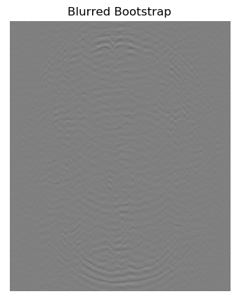 Figure 1
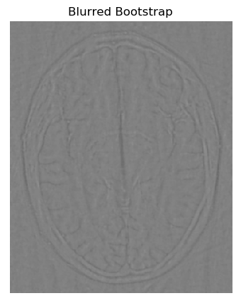 Figure 2
 Figure 3
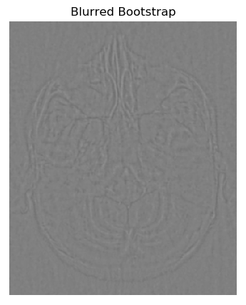 Figure 4
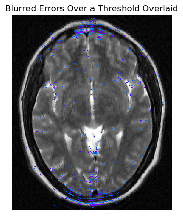 Figure 5
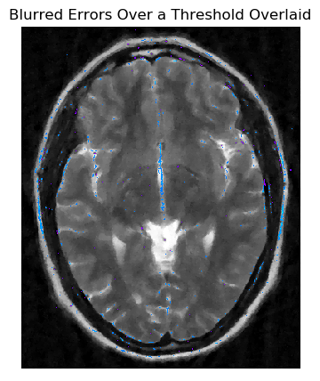 Figure 6
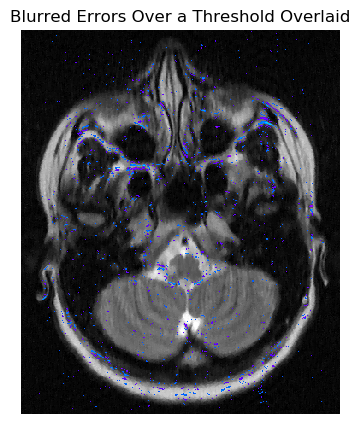 Figure 7
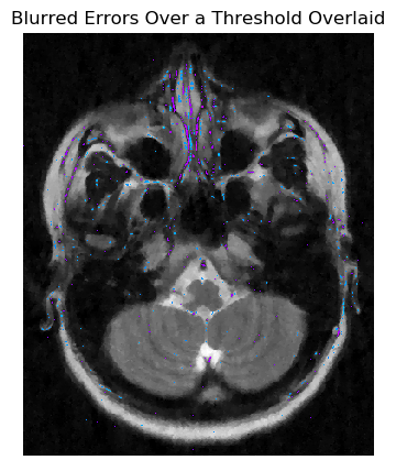 Figure 8
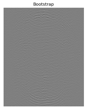 Figure 9
 Figure 10
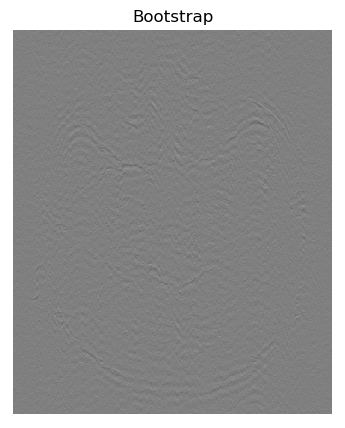 Figure 11
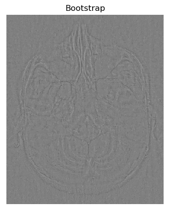 Figure 12
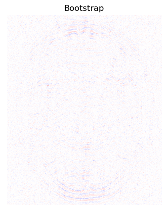 Figure 13
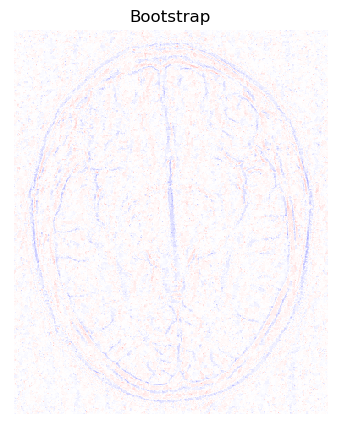 Figure 14
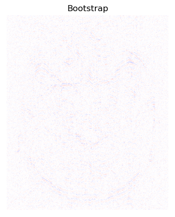 Figure 15
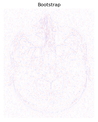 Figure 16
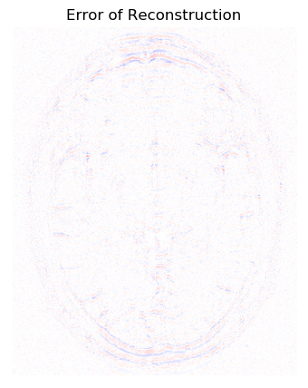 Figure 17
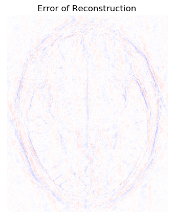 Figure 18
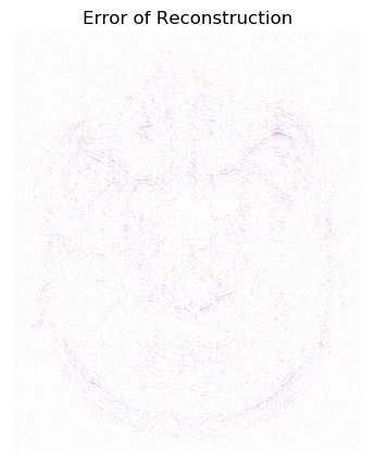 Figure 19
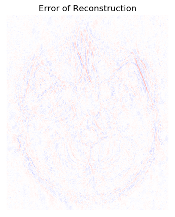 Figure 20
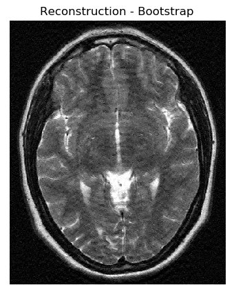 Figure 21
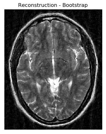 Figure 22
 Figure 23
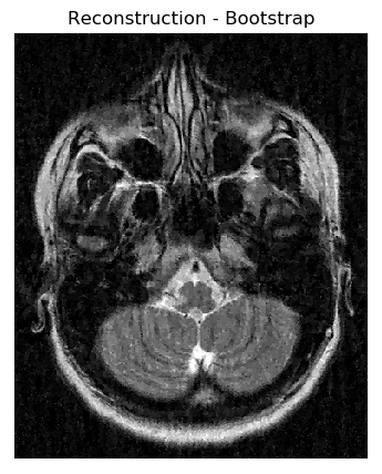 Figure 24
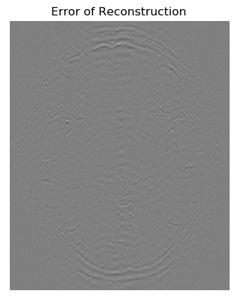 Figure 25
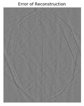 Figure 26
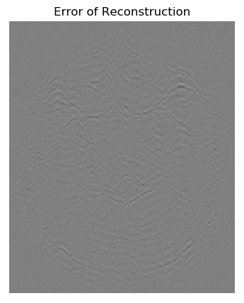 Figure 27
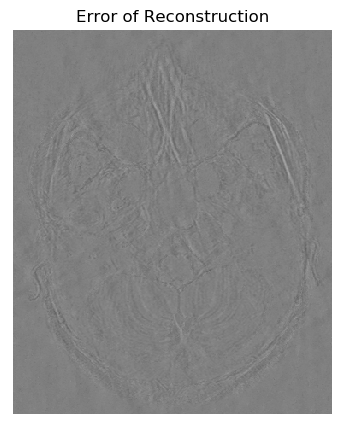 Figure 28
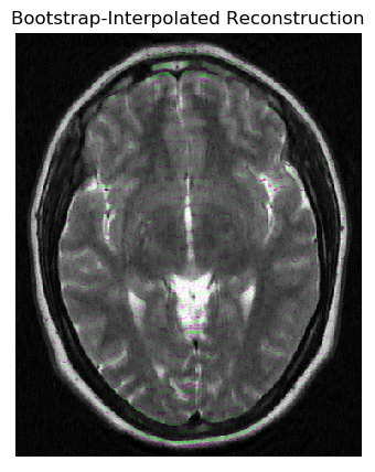 Figure 29
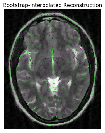 Figure 30
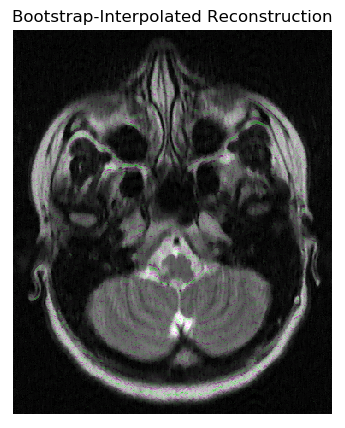 Figure 31
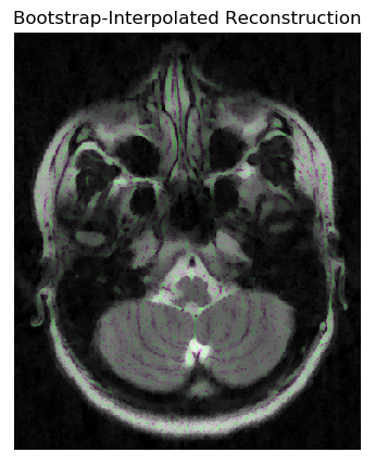 Figure 32
 Figure 33
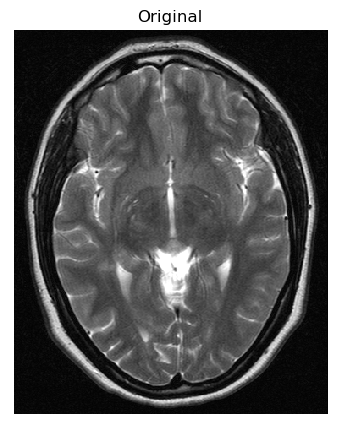 Figure 34
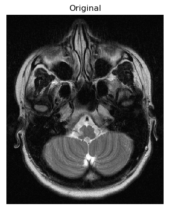 Figure 35
 Figure 36
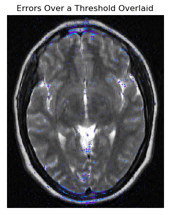 Figure 37
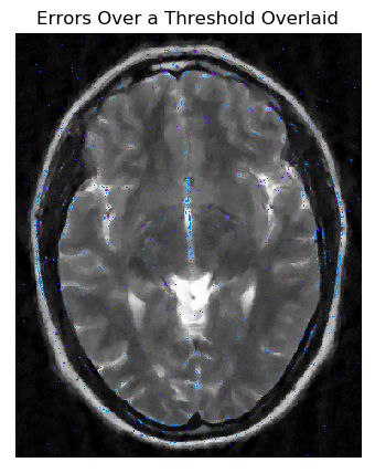 Figure 38
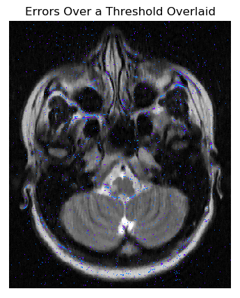 Figure 39
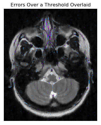 Figure 40
| Sampling | Slice | Bootstrap | Blurred Bootstrap |
|---|---|---|---|
| horizontally | lower | 12.9 | 6.25 |
| horizontally | upper | 13.8 | 7.34 |
| radially | lower | 17.5 | 10.5 |
| radially | upper | 18.0 | 11.6 |
| Std. Dev. | Horizontally | Radially |
|---|---|---|
| 0.0 | 12.9 | 17.5 |
| 0.5 | 9.94 | 14.6 |
| 1.0 | 6.25 | 10.5 |
| 1.5 | 4.38 | 8.06 |
| 2.0 | 3.03 | 6.34 |
| 2.5 | 2.04 | 5.06 |
| 3.0 | 1.33 | 4.09 |
| 3.5 | .847 | 3.34 |
| 4.0 | .535 | 2.75 |
| Std. Dev. | Horizontally | Radially |
|---|---|---|
| 0.0 | 13.8 | 18.0 |
| 0.5 | 10.9 | 15.3 |
| 1.0 | 7.34 | 11.6 |
| 1.5 | 5.35 | 9.50 |
| 2.0 | 3.82 | 7.97 |
| 2.5 | 2.63 | 6.79 |
| 3.0 | 1.75 | 5.87 |
| 3.5 | 1.14 | 5.13 |
| 4.0 | .745 | 4.54 |
Peer Reviews
No public reviews on file for this paper yet. If you reviewed it on a platform where reviews are public (OpenReview, ICLR, NeurIPS, ICML), you can paste yours below so the community can read it here.
Videos
No videos yet. Explain this paper in a talk, walkthrough, or lecture? Add one.
Taxonomy
TopicsMedical Imaging Techniques and Applications · Photoacoustic and Ultrasonic Imaging · Sparse and Compressive Sensing Techniques
Methods of interpreting error estimates
for grayscale image reconstructions
Aaron Defazio and Mark Tygert
Abstract
One representation of possible errors in a grayscale image reconstruction is as another grayscale image estimating potentially worrisome differences between the reconstruction and the actual “ground-truth” reality. Visualizations and summary statistics can aid in the interpretation of such a representation of error estimates. Visualizations include suitable colorizations of the reconstruction, as well as the obvious “correction” of the reconstruction by subtracting off the error estimates. The canonical summary statistic would be the root-mean-square of the error estimates. Numerical examples involving cranial magnetic-resonance imaging clarify the relative merits of the various methods in the context of compressed sensing. Unfortunately, the colorizations appear likely to be too distracting for actual clinical practice, and the root-mean-square gets swamped by background noise in the error estimates. Fortunately, straightforward displays of the error estimates and of the “corrected” reconstruction are illuminating, and the root-mean-square improves greatly after mild blurring of the error estimates; the blurring is barely perceptible to the human eye yet smooths away background noise that would otherwise overwhelm the root-mean-square.
1 Introduction
Compressed sensing in imaging is a paradigm for accelerating the acquisition of full images by taking fewer measurements than the number of degrees of freedom being reconstructed. The measurements are thus “undersampled” relative to the usual information-theoretic requirements of sampling at the Nyquist rate etc. Compressed sensing therefore risks introducing errors, errors which very well may vary among different image acquisitions. Recent work of [Tygert et al., 2018] and others generates an error “bar” for each reconstructed image, in the form of another image that can be expected to be representative of potential differences between the reconstruction and the real ground-truth. The present paper considers user-friendly methods for generating visualizations and automatic interpretations of these error estimates, appropriate for display to medical professionals (especially radiologists) on data of cranial scans from magnetic-resonance imaging (MRI) machines.
After testing several natural visual displays, we find that any nontrivial visualization is likely to be too distracting for physicians, as some have expressed reservations about having to look at any errors at all — they would be much happier having a machine look at the estimates and flag potentially serious errors for special consideration. We might conclude that colorization is too distracting, that the best visualizations are simple displays of the error estimates, possibly supplemented with the error estimates subtracted from the reconstructions (thus showing how the error estimates can “correct” the reconstructions). Most of the results of the present paper about visualization could be regarded as negative, however natural and straightforward the colorizations may be.
For circumstances in which visualizing errors is overkill (or unnecessarily bothersome), we find that an almost simplistic automated interpretation of the plots of errors — reporting just the root-mean-square of the denoised error estimates — works remarkably well. While background noise dominates the root-mean-square of the initial, noisy error estimates, even denoising that is almost imperceptible can remove the obfuscatory background noise; the root-mean-square can then focus on the remaining errors, which are often relatively sparsely distributed. When the root-mean-square of the denoised error estimates is large enough, a clinician could look at the visualizations mentioned above to fully understand the implications of the error estimates (or rescan the patient using a less error-prone sampling pattern).
2 Methods
2.1 Visualization in grayscale and in color
We include four kinds of plots displaying the full reconstructions and errors:
“Original” is the original grayscale image. 2. 2.
“Reconstruction” is the reconstruction via compressed sensing. Specifically, we use the configuration of [Tygert et al., 2018]; for details (which are largely irrelevant for comparing the utility of visualizations), please see the third section, “Numerical examples,” of [Tygert et al., 2018]. 3. 3.
“Error of Reconstruction” displays the difference between the original and reconstructed images, with black (or white) corresponding to extreme errors, and middling grays corresponding to the absence of errors. 4. 4.
“Bootstrap” displays the errors estimated via the bootstrap of [Tygert et al., 2018] (using the same 1000 iterations used by [Tygert et al., 2018]), with black (or white) corresponding to extreme errors, and middling grays corresponding to the absence of errors.
We visualize the errors in reconstruction and the bootstrap estimates using grayscale so that the phases of oscillatory artifacts are less apparent; colorized errors look very different for damped sine versus cosine waves, whereas the medical meaning of such waves is often similar. Appendix A displays the errors in color.
We consider four methods for visualizing the effects of errors (as estimated via the bootstrap) simultaneously with displaying the reconstruction, via manipulation of the hue-saturation-value color space described, for example, by [van der Walt et al., 2014]:
“Reconstruction - Bootstrap” is literally the bootstrap error estimate subtracted from the reconstruction, in some sense “correcting” or “enhancing” the reconstruction. 2. 2.
“Errors Over a Threshold Overlaid” identifies the pixels in the bootstrap error estimate whose absolute values are in the upper percentiles (the upper two percentiles for horizontally retained sampling, the upper one for radially retained sampling), then replaces those pixels (retaining all other pixels unchanged) in the reconstruction with colors corresponding to the values of the pixels in the bootstrap. Specifically, the colors plotted are at the highest value possible and fully saturated, with a hue ranging from cyan to magenta, with blue in the middle (however, as we include only the upper percentiles, only hues very close to cyan or to magenta actually get plotted). This effectively marks the pixels corresponding to the largest estimated errors with eye-popping colors, leaving the other pixels at their gray values in the reconstruction. 3. 3.
“Bootstrap-Saturated Reconstruction” sets the saturation of a pixel in the reconstruction to the corresponding absolute value of the pixel in the bootstrap error estimate (normalized by the greatest absolute value of any pixel in the bootstrap), with a hue set to red or green depending on the sign of the pixel in the bootstrap. The value of the pixel in the reconstruction stays the same. Thus, a pixel gets colored more intensely red or more intensely green when the absolute value of the pixel in the bootstrap is large, but always with the value in hue-saturation-value remaining the same as in the original reconstruction; a pixel whose corresponding absolute value in the bootstrap is relatively negligible stays unsaturated gray at the value in the reconstruction. 4. 4.
“Bootstrap-Interpolated Reconstruction” leaves the value of each pixel at its value in the reconstruction, and linearly interpolates in the hue-saturation plane between green and magenta based on the corresponding value of the pixel in the bootstrap error estimate (normalized by the greatest absolute value of any pixel in the bootstrap). Pure gray is in the middle of the line between green and magenta, so that any pixel whose corresponding error estimate is zero will appear unchanged, exactly as it was in the original reconstruction; pixels whose corresponding error estimates are the largest have the same value as in the reconstruction but get colored magenta, while those whose corresponding error estimates are the most negative have the same value as in the reconstruction but get colored green.
2.2 Summarization in a scalar
The square root of the sum of the squares of slightly denoised error estimations summarizes in a single scalar the overall size of errors. Even inconspicuous denoising can greatly improve the root-mean-square: While the effect of blurring the bootstrap error estimates with a normalized Gaussian convolutional kernel of standard deviation one pixel is almost imperceptible to the human eye (or at least preserves the semantically meaningful structures in the images), the blur helps remove the background of noise that can otherwise dominate the root-mean-square of the error estimates. The blur largely preserves significant edges and textured areas, yet can eliminate much of the perceptually immaterial zero-mean background noise. Whereas background noise can overwhelm the root-mean-square of the initial, noisy bootstrap, the root-mean-square of the slightly blurred bootstrap captures the magnitude of the important features in the error estimates.
3 Results
Our data comes from [Loizou et al., 2013a], [Loizou et al., 2011], [Loizou et al., 2013b], [Loizou et al., 2015]. Specifically, we consider two cross-sectional slices through the head of a patient in an MRI scanner: the lower slice is the third of twenty from [Tygert et al., 2018], while the upper slice is the tenth of twenty from [Tygert et al., 2018]. Compressed sensing reconstructs a cross-sectional image given only a subset of the usual measurements of values of the two-dimensional Fourier transform of the original, “ground-truth” cross-section. We consider the radially retained and horizontally retained subsets of [Tygert et al., 2018], which yield the error estimates displayed in the figures below (the third section, “Numerical examples,” of [Tygert et al., 2018] details the schemes for sampling, but these details are irrelevant for assessment of visualizations). We used the Python package (“fbooja”) of [Tygert et al., 2018]; the Gaussian blur from Subsection 2.2 leverages skimage.filters.gaussian from scikit-image of [van der Walt et al., 2014].
Figures 1–8 display the visualizations from Subsection 2.1. Figures 9 and 10 depict the effects of the Gaussian blur from Subsection 2.2. Table 1 reports how drastically such a nearly imperceptible blur changes the square roots of the sums of the squares of the error estimates. Background noise clearly overwhelms the root-mean-square without any denoising of the error estimates — the root-mean-square decreases dramatically even with just the mild denoising of blurring with a normalized Gaussian convolutional kernel whose standard deviation is one pixel, as in Table 1 and Figures 9 and 10. Tables 2 and 3 report how blurring with wider Gaussians affects the root-mean-square; of course, wider Gaussian blurs are much more conspicuous and risk washing out important coherent features of the error estimates, while the last column of Table 3 shows that denoising with wider Gaussian blurs brings diminishing returns. The width used in Table 1 and Figures 9 and 10 — only one pixel — may be safest. Appendix B displays the grayscale reconstructions overlaid with the blurred bootstraps (blurring with a Gaussian whose standard deviation is one pixel), thresholded and colorized as in Subsection 2.1.
4 Discussion and Conclusion
Broadly speaking, the bootstrap-saturated reconstructions and bootstrap-interpolated reconstructions look similar, even though the details of their constructions differ. Both the bootstrap-saturated reconstruction and the bootstrap-interpolated reconstruction highlight errors more starkly on pixels for which the reconstruction is bright; dark green, dark red, and dark magenta (that is, with a relatively low value in hue-saturation-value) simply do not jump out visually, even if the green, red, or magenta are fully saturated. That said, retaining the value of the pixel in the reconstruction makes the colorization of the bootstrap-saturated reconstruction and the bootstrap-interpolated reconstruction far less distracting than in errors over a threshold overlaid, with much higher fidelity to the form of the grayscale reconstruction in the colored regions. Of course, the errors over a threshold overlaid do not alter the grayscale reconstruction at all when the errors are within the threshold, so the fidelity to the grayscale reconstruction is perfect in those areas of the images with overlaid errors where the error estimates do not go beyond the threshold.
Thus, none of the colorizations is uniformly superior to the others, and all may be too distracting for actual clinical practice. Alternatives include direct display of the bootstrap error estimates, possibly complemented by the bootstrap subtracted from the reconstruction (to illustrate the effects of “correcting” the reconstruction with the error estimates), which are readily interpretable and minimally distracting.
The bootstrap subtracted from the reconstruction tends to sharpen the reconstruction and to add back some features such as lines or textures that the reconstruction obscured. However, this reconstruction that is “corrected” with the bootstrap estimations may contain artifacts not present in the original image — the error estimates tend to be conservative, possibly suspecting errors in some regions where in fact the reconstruction is accurate. The “corrected” reconstruction (that is, the bootstrap subtracted from the reconstruction) can be illuminating, but only as a complement to plotting the bootstrap error estimates on their own, too.
A sensible protocol could be to check if the root-mean-square of the blurred bootstrap is large enough to merit further investigation, investigating further by looking at the full bootstrap image together with the reconstruction “corrected” by subtracting off the bootstrap error estimates (or colorizations).
Appendix A Bootstraps and Errors in Color
For reference, this appendix displays the errors of reconstruction and bootstrap estimates in color, with blue for negative errors, red for positive errors, and white for the absence of any error (light blue and light red indicate less extreme errors than pure blue or pure red). The labeling conventions (“lower,” “upper,” etc.) conform to those introduced in Section 3.
Appendix B Blurred Errors Over a Threshold Overlaid
For reference, this appendix displays the same errors over a threshold overlaid over the reconstruction as in Subsection 2.1, together with the blurred errors over a threshold overlaid over the reconstruction (blurring with a Gaussian convolutional kernel whose standard deviation is one pixel, as in Subsection 2.2). The labeling conventions (“lower,” “upper,” etc.) conform to those introduced in Section 3. The blurred errors certainly introduce less distracting noise than without blurring, yet the colors still appear really distracting.
The reference list from the paper itself. Each links out to its DOI / PubMed record.
- 1[Loizou et al., 2013 a] Loizou, C. P., Kyriacou, E. C., Seimenis, I., Pantziaris, M., Petroudi, S., Karaolis, M., and Pattichis, C. (2013 a). Brain white matter lesion classification in multiple sclerosis subjects for the prognosis of future disability. Intel. Decision Tech. J. , 7:3–10.
- 2[Loizou et al., 2011] Loizou, C. P., Murray, V., Pattichis, M., Seimenis, I., Pantziaris, M., and Pattichis, C. (2011). Multi-scale amplitude-modulation–frequency-modulation (AM-FM) texture analysis of multiple sclerosis in brain MRI images. IEEE Trans. Inform. Tech. Biomed. , 15(1):119–129.
- 3[Loizou et al., 2013 b] Loizou, C. P., Pantziaris, M., Pattichis, C. S., and Seimenis, I. (2013 b). Brain MRI image normalization in texture analysis of multiple sclerosis. J. Biomed. Graph. Comput. , 3(1):20–34.
- 4[Loizou et al., 2015] Loizou, C. P., Petroudi, S., Seimenis, I., Pantziaris, M., and Pattichis, C. (2015). Quantitative texture analysis of brain white matter lesions derived from T 2-weighted MR images in MS patients with clinically isolated syndrome. J. Neuroradiol. , 42(2):99–114.
- 5[Tygert et al., 2018] Tygert, M., Ward, R., and Zbontar, J. (2018). Compressed sensing with a jackknife and a bootstrap. Technical Report 1809.06959, ar Xiv.
- 6[van der Walt et al., 2014] van der Walt, S., Schönberger, J. L., Nunez-Iglesias, J., Boulogne, F., Warner, J. D., Yager, N., Gouillart, E., and Yu, T. (2014). Scikit-image: image processing in Python. Peer J , 2(e 453):1–18.