A Sequential Two-Step Algorithm for Fast Generation of Vehicle Racing Trajectories
Nitin R. Kapania, John Subosits, J Christian Gerdes

TL;DR
This paper introduces a fast, iterative two-step algorithm for real-time vehicle racing trajectory generation that balances computational efficiency with near-optimal lap times, validated on an autonomous racecar.
Contribution
The paper presents a novel two-step iterative approach that simplifies nonlinear optimal control into convex subproblems for rapid trajectory planning.
Findings
Converges in 4-5 iterations with 30 seconds per full lap computation.
Achieves lap times comparable to nonlinear optimization and professional drivers.
Validated on an autonomous Audi TTS at Thunderhill Raceway.
Abstract
The problem of maneuvering a vehicle through a race course in minimum time requires computation of both longitudinal (brake and throttle) and lateral (steering wheel) control inputs. Unfortunately, solving the resulting nonlinear optimal control problem is typically computationally expensive and infeasible for real-time trajectory planning. This paper presents an iterative algorithm that divides the path generation task into two sequential subproblems that are significantly easier to solve. Given an initial path through the race track, the algorithm runs a forward-backward integration scheme to determine the minimum-time longitudinal speed profile, subject to tire friction constraints. With this fixed speed profile, the algorithm updates the vehicle's path by solving a convex optimization problem that minimizes the resulting path curvature while staying within track boundaries and…
Click any figure to enlarge with its caption.
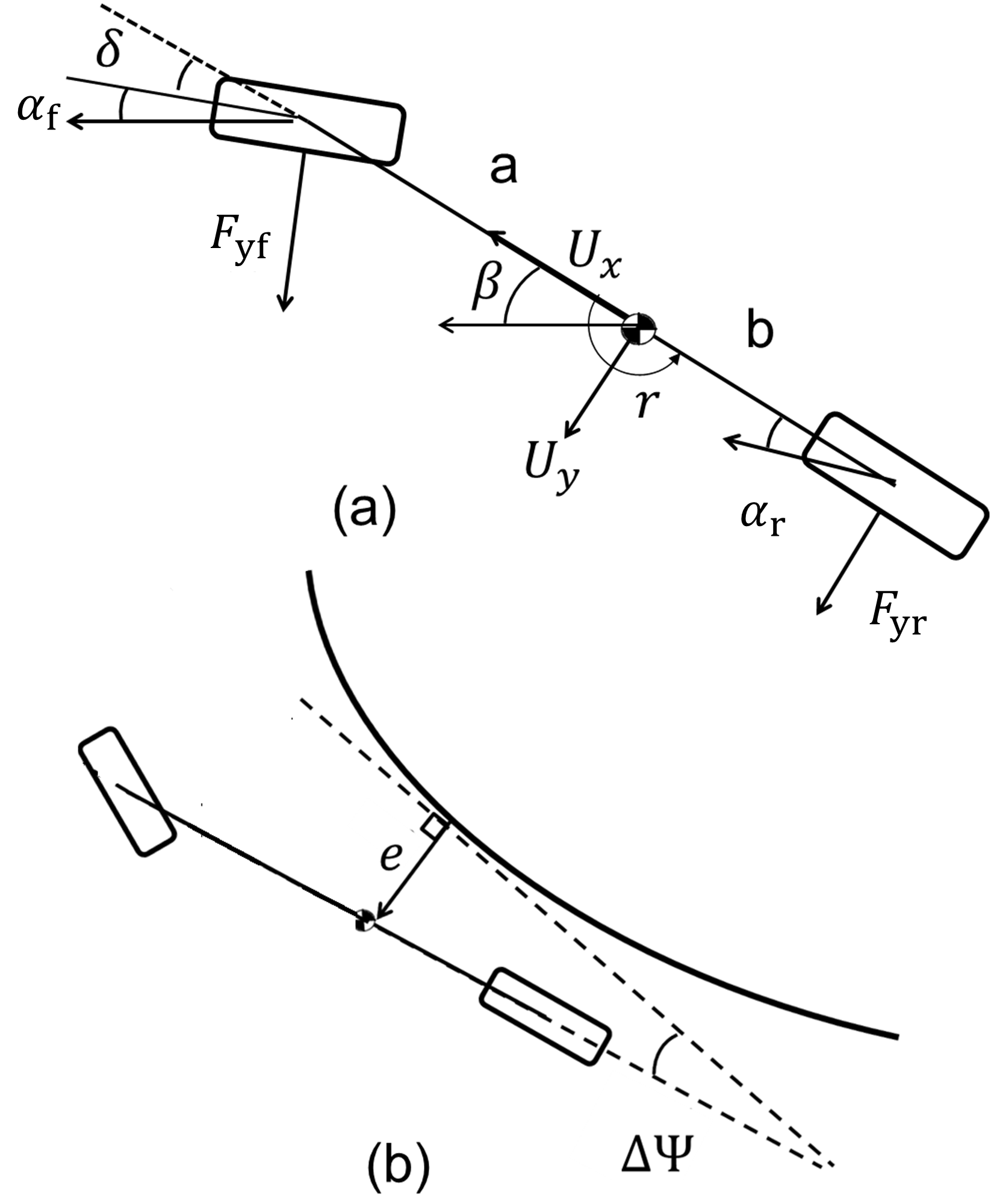 Figure 1
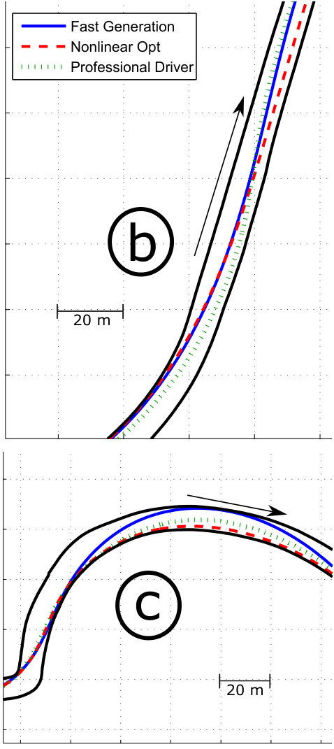 Figure 2
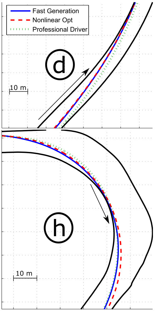 Figure 3
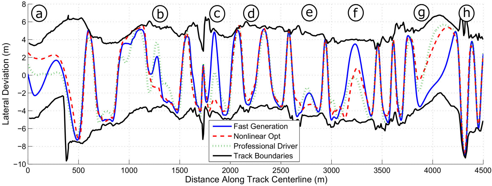 Figure 4
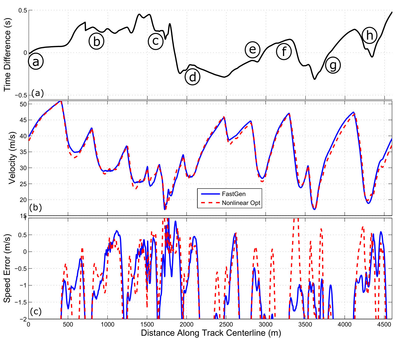 Figure 5
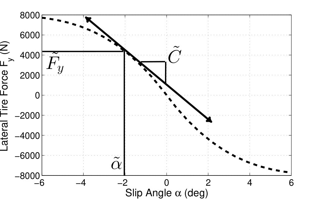 Figure 6
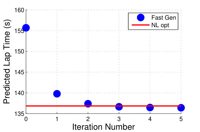 Figure 7
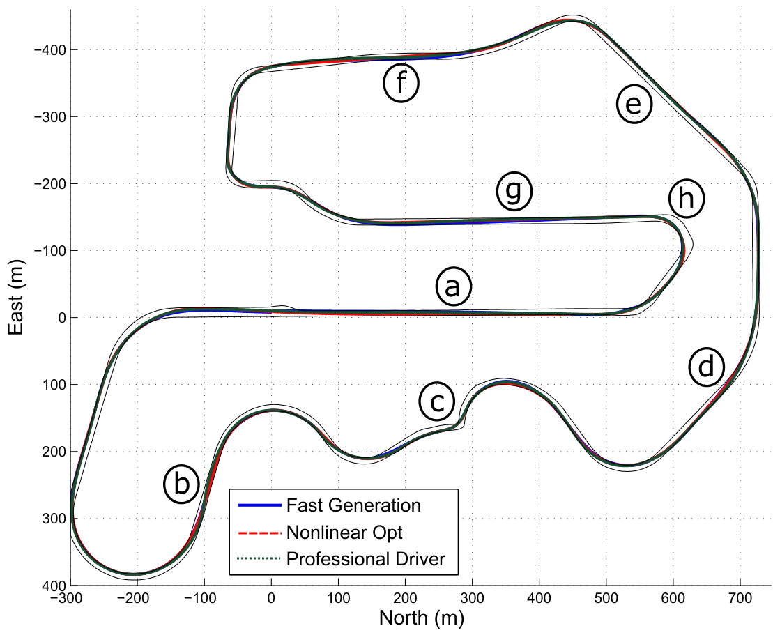 Figure 8
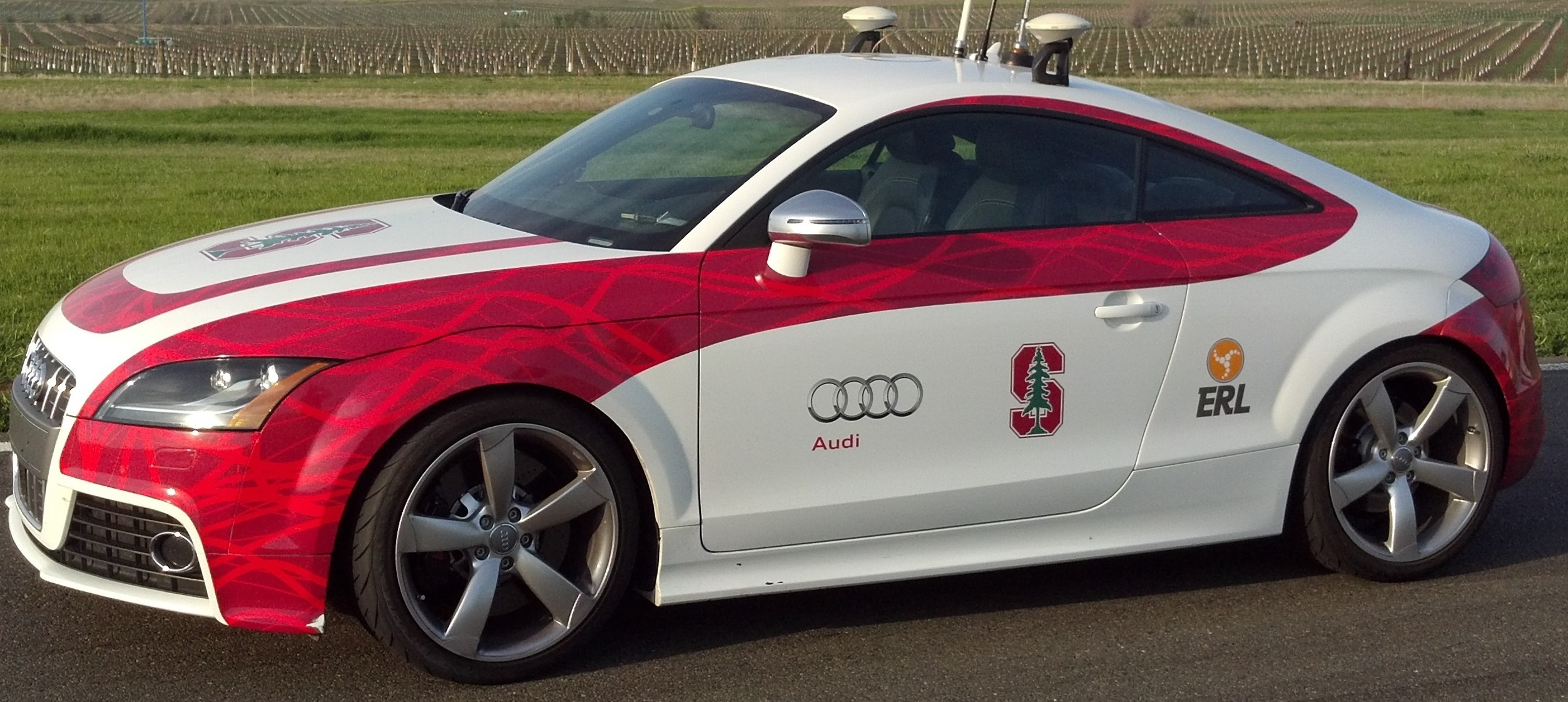 Figure 9
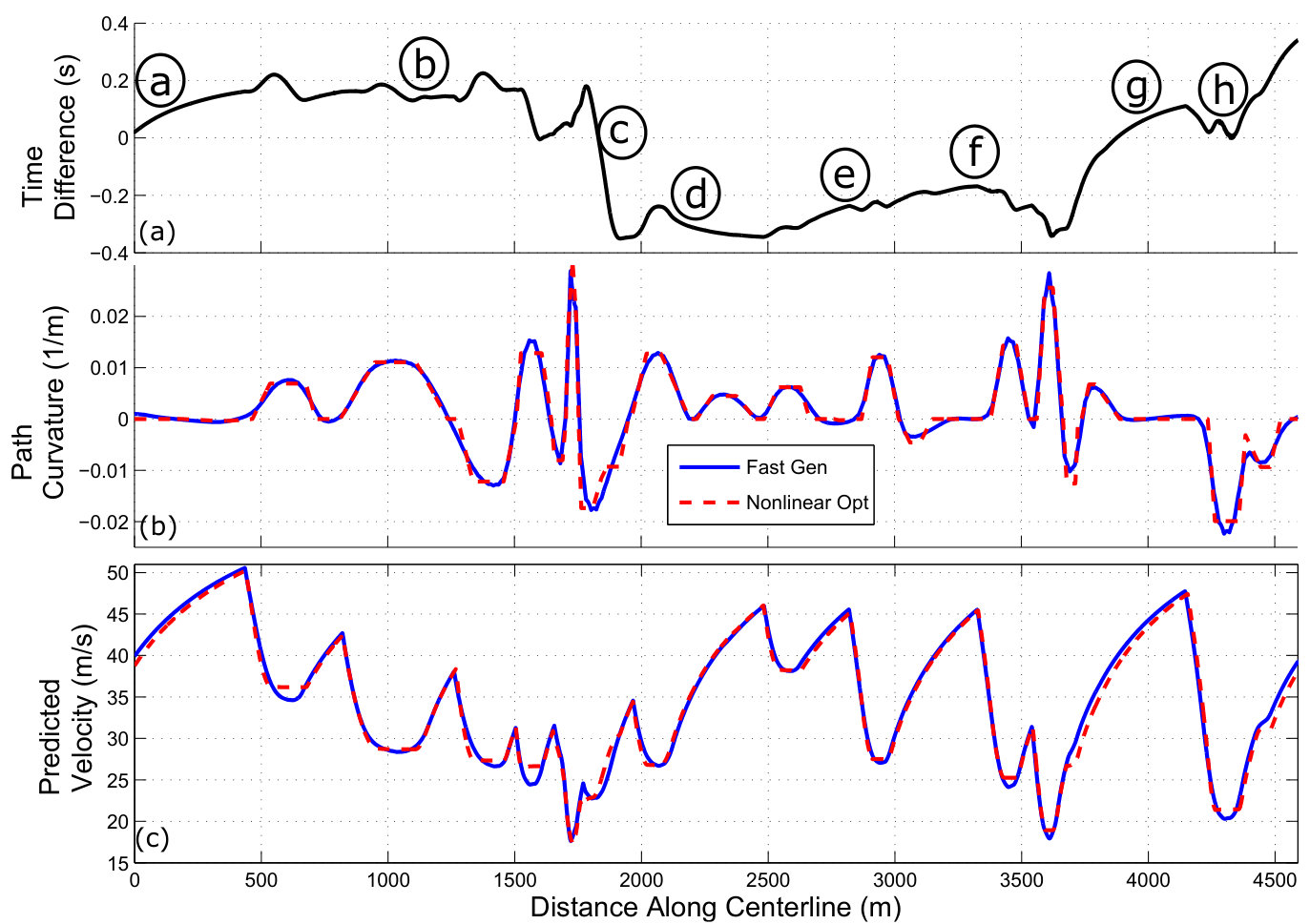 Figure 10
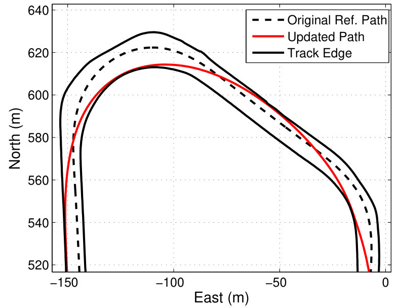 Figure 11
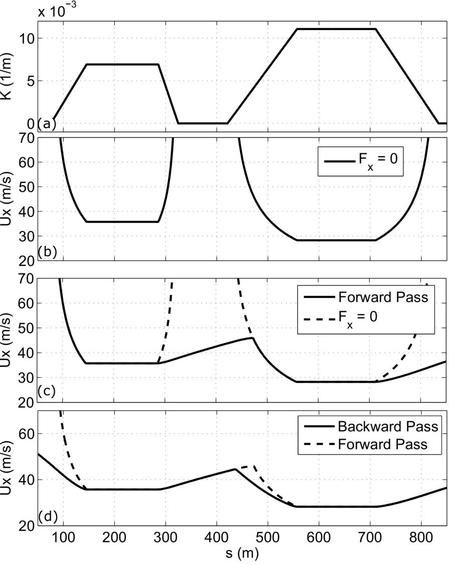 Figure 12
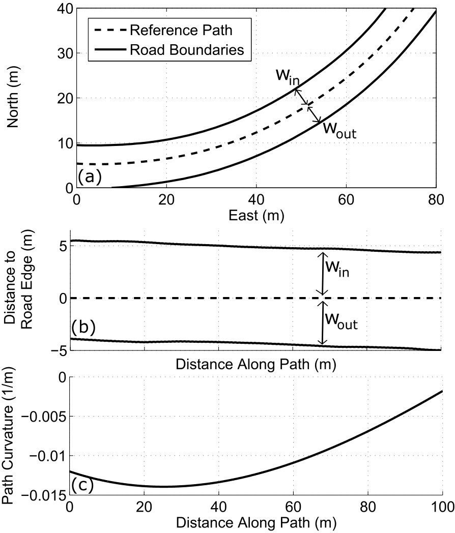 Figure 13
| Parameter | Symbol | Value | Units |
|---|---|---|---|
| Regularization Parameter | 1 | ||
| Stop Criterion | .1 | s | |
| Vehicle mass | 1500 | kg | |
| Yaw Inertia | 2250 | ||
| Front axle to CG | 1.04 | m | |
| Rear axle to CG | 1.42 | m | |
| Front cornering stiffness | 160 | ||
| Rear cornering stiffness | 180 | ||
| Friction Coefficient | 0.95 | ||
| Path Discretization | 2.75 | ||
| Optimization Time Steps | 1843 | - | |
| Max Engine Force | - | 3750 | N |
| Simulation | Experiment | |
|---|---|---|
| Fast Generation | 136.4 | 138.6 |
| Gradient Descent | 136.7 | 139.2 |
| Human Driver | N/A | 137.7 |
| Lookahead (m) | Solve Time (s) | |
|---|---|---|
| 450 | 184 | 5 |
| 900 | 369 | 6 |
| 1800 | 737 | 12 |
| 4500 | 1843 | 26 |
Peer Reviews
No public reviews on file for this paper yet. If you reviewed it on a platform where reviews are public (OpenReview, ICLR, NeurIPS, ICML), you can paste yours below so the community can read it here.
Videos
No videos yet. Explain this paper in a talk, walkthrough, or lecture? Add one.
A Sequential Two-Step Algorithm for Fast Generation of Vehicle Racing Trajectories
Nitin R. Kapania Address all correspondence to this author.
Dept. of Mechanical Engineering
Stanford University
Stanford, CA 94305
John Subosits
Dept. of Mechanical Engineering
Stanford University
Stanford, CA 94305
J. Christian Gerdes
Dept. of Mechanical Engineering
Stanford University
Stanford, CA 94305
Abstract
The problem of maneuvering a vehicle through a race course in minimum time requires computation of both longitudinal (brake and throttle) and lateral (steering wheel) control inputs. Unfortunately, solving the resulting nonlinear optimal control problem is typically computationally expensive and infeasible for real-time trajectory planning. This paper presents an iterative algorithm that divides the path generation task into two sequential subproblems that are significantly easier to solve. Given an initial path through the race track, the algorithm runs a forward-backward integration scheme to determine the minimum-time longitudinal speed profile, subject to tire friction constraints. With this fixed speed profile, the algorithm updates the vehicle’s path by solving a convex optimization problem that minimizes the resulting path curvature while staying within track boundaries and obeying affine, time-varying vehicle dynamics constraints. This two-step process is repeated iteratively until the predicted lap time no longer improves. While providing no guarantees of convergence or a globally optimal solution, the approach performs very well when validated on the Thunderhill Raceway course in Willows, CA. The predicted lap time converges after four to five iterations, with each iteration over the full 4.5 km race course requiring only thirty seconds of computation time on a laptop computer. The resulting trajectory is experimentally driven at the race circuit with an autonomous Audi TTS test vehicle, and the resulting lap time and racing line is comparable to both a nonlinear gradient descent solution and a trajectory recorded from a professional racecar driver. The experimental results indicate that the proposed method is a viable option for online trajectory planning in the near future.
1 Introduction
The problem of calculating the minimum lap time trajectory for a given vehicle and race track has been studied over the last several decades in the control, optimization, and vehicle dynamics communities. Early research by Hendrikx et al. [1] in 1996 used Pontryagin’s minimum principle to derive coupled differential equations to solve for the minimum-time trajectory of a vehicle lane change maneuver. The minimum lap time problem drew significant interest from professional racing teams, and Casanova [2] published a method in 2000 capable of simultaneously optimizing both the path and speed profile for a fully nonlinear vehicle model using nonlinear programming (NLP). Kelly [3] further extended the results from Casanova by considering the physical effect of tire thermodynamics and applying more robust NLP solution methods such as Feasible Sequential Quadratic Programming. More recently, Perantoni and Limebeer [4] showed that the computational expense could be significantly reduced by applying curvilinear track coordinates, non-stiff vehicle dynamics, and the use of smooth computer-generated analytic derivatives. The authors simulated the optimal vehicle lap on the Catalunya race circuit with a spatial discretization of two meters and a solve time of around 15 minutes.
More recently, the development of autonomous vehicle technology at the industry and academic level has led to research on optimal path planning algorithms that can be used for driverless cars. Theodosis and Gerdes published a gradient descent approach for determining time-optimal racing lines, with the racing line constrained to be composed of a fixed number of clothoid segments [5]. Given the computational expense of performing nonlinear optimization, there has also been a significant research effort to find approximate methods that provide fast lap times. Timings and Cole [6] formulated the minimum lap time problem into a model predictive control (MPC) problem by linearizing the nonlinear vehicle dynamics at every time step and approximating the minimum-time objective by maximizing distance traveled along the path centerline. The resulting racing line for a 90 degree turn was simulated next to an NLP solution. Gerdts et al. [7] proposed a similar receding horizon approach, where distance along a reference path was maximized over a series of locally optimal optimization problems that were combined with continuity boundary conditions. One potential drawback of the model predictive control approach is that an optimization problem must be reformulated and solved at every time step, which can still be computationally expensive. For example, Timings and Cole reported a computation time of 900 milliseconds per 20 millisecond simulation step with the CPLEX quadratic program solver on a desktop PC.
While experimental validation was reported only by [5] and [7], all of the aforementioned methods are feasible for experimental implementation, as an autonomous vehicle can apply a closed-loop controller to follow a time-optimal vehicle trajectory computed offline. However, there are significant benefits to developing a fast trajectory generation algorithm that can approximate the globally optimal trajectory in real-time. If the algorithm runtime is small compared to the actual lap time, the algorithm can run as a real-time trajectory planner and find a fast racing line for the next several turns of the racing circuit. This would allow the trajectory planner to modify the desired path based on the motion of competing race vehicles and estimates of road friction, tire wear, engine/brake dynamics and other parameters learned over several laps of racing. Additionally, the fast trajectory algorithm can be used to provide a very good initial trajectory for a nonlinear optimization method.
This paper therefore presents an experimentally validated iterative algorithm that generates vehicle racing trajectories with low computational expense. To decrease computation time, the combined lateral/longitudinal optimal control problem is replaced by two sequential sub-problems where minimum-time longitudinal speed inputs are computed given a fixed vehicle path, and then the vehicle path is updated given the fixed speed commands.
The following section presents a mathematical framework for the trajectory generation problem and provides a linearized five-state model for the planar dynamics of a racecar following a set of speed and steering inputs, with lateral and heading error states computed with respect to a fixed path. Section 3 describes the method of finding the minimum-time speed inputs given a fixed path. While this task has been recently formulated as a convex optimization problem [8], a forward-backward integration scheme based on prior work [9] is used instead. Section 4 describes a method for updating the racing path given the fixed speed inputs using convex optimization, where the curvature norm of the driven path is explicitly minimized. The complete algorithm is outlined in Section 5, and the racing trajectory generated on the Thunderhill Raceway circuit in Willows, CA is compared to results from both a nonlinear optimization and data recorded from a professional racecar driver. In Section 6, the racing trajectory is then tested experimentally in an autonomous Audi TTS testbed via a previously published closed-loop path following controller [10]. The resulting lap time compares well with the lap time recorded for the nonlinear optimization trajectory. Section 7 concludes by discussing future implementation of the algorithm in a real-time path planner.
2 Path Description and Vehicle Model
Figure 1 describes the parameterization of the reference path that the vehicle will follow. The reference path is most intuitively described in Fig. 1(a) as a smooth curve of Cartesian East-North coordinates, with road boundaries represented by similar Cartesian curves. However, for the purposes of quickly generating a racing trajectory, it is more convenient to parameterize the reference path as a curvature profile that is a function of distance along the path (Fig. 1(c)). Additionally, it is convenient to store the road boundary information as two functions and , which correspond to the lateral distance from the path at to the inside and outside road boundaries, respectively (Fig. 1(b)). This maximum lateral distance representation will be useful when constraining the generated racing path to lie within the road boundaries. The transformation from the local , coordinate frame to the global Cartesian coordinates , are given by the Fresnel integrals:
[TABLE]
where is the heading angle of the reference path and is a dummy variable.
With the reference path defined in terms of and , the next step is to define the dynamic model of the vehicle. For the purposes of trajectory generation, we assume the vehicle dynamics are given by the planar bicycle model in Fig. 2(a), with yaw rate and sideslip states describing the lateral dynamics. Additionally, the vehicle’s offset from the reference path is given by the path lateral deviation state and path heading error state (Fig. 2(b)). Linearized equations of motion for all four states are given by:
[TABLE]
where is the vehicle forward velocity and and are the front and rear lateral tire forces. The vehicle mass and yaw inertia are denoted by and , and the geometric parameters and are shown in Fig. 2(a). Note that while the vehicle longitudinal dynamics are not explicitly modeled, the bicycle model does allow for time-varying values of .
3 Velocity Profile Generation Given Fixed Reference Path
Given a fixed reference path described by and , the first algorithm step is to find the minimum-time speed profile the vehicle can achieve without exceeding the available tire-road friction. The approach taken in this paper is a “three-pass” approach described in complete detail by Subosits and Gerdes [9], and originally inspired by work from Velenis and Tsiotras [11]. Given the lumped front and rear tires from Fig. 2(a), the available longitudinal force and lateral force at each wheel is constrained by the friction circle:
[TABLE]
where is the tire-road friction coefficient and is the available normal force. The first pass of the speed profile generation aims to find the maximum permissible steady state vehicle speed given zero longitudinal force. For the simplified case where weight transfer and topography effects are neglected, this is given by:
[TABLE]
where the result in (4) is obtained by setting and . The results of this first pass for the sample curvature profile in Fig. 3(a) are shown in Fig. 3(b). The next step is a forward integration step, where the velocity of a given point is determined by the velocity of the previous point and the available longitudinal force for acceleration. This available longitudinal force is calculated in [9] by accounting for the vehicle engine force limit and the lateral force demand on all tires due to the road curvature:
[TABLE]
A key point of the forward integration step is that at every point, the value of is compared to the corresponding value from (4), and the minimum value is taken. The result is shown graphically in Fig. 3(c). Finally, the backward integration step occurs, where the available longitudinal force for deceleration is again constrained by the lateral force demand on all tires:
[TABLE]
The value of is then compared to the corresponding value from (5) for each point along the path, and the minimum value is chosen, resulting in the final velocity profile shown by the solid line in Fig. 3(d). While treatment of three-dimensional topography effects are not described in this paper, the method described in [9] and used for the experimental data collection determines the normal and lateral tire forces and at each point along the path by accounting for weight transfer, road bank and grade.
4 Updating Path Given Fixed Velocity Profile
4.1 Overall Approach and Minimum Curvature Heuristic
The second step of the trajectory generation algorithm takes the original reference path and corresponding velocity profile as inputs, and modifies the reference path to obtain a new, ideally faster, racing line. Sharp [12] suggests a general approach for modifying an initial path to obtain a faster lap time by taking the original path and velocity profile and incrementing the speed uniformly by a small, constant “learning rate.” An optimization problem is then solved to find a new reference path and control inputs that allow the vehicle to drive at the higher speeds without driving off the road. If a crash is detected, the speed inputs are locally reduced around the crash site and the process is repeated.
However, one challenge with this approach is that it can take several hundred iterations of locally modifying the vehicle speed profile, detecting crashes, and modifying the reference path to converge to a fast lap time. An alternative approach is to modify the reference path in one step by solving a single optimization problem. The lap time for a given racing line is provided by the following equation:
[TABLE]
Equation (7) implies that minimizing the vehicle lap time requires simultaneously minimizing the total path length while maximizing the vehicle’s longitudinal velocity . These are typically competing objectives, as lower curvature (i.e. higher radius) paths can result in longer path lengths but higher vehicle speeds when the lateral force capability of the tires is reached, as shown in (4). As mentioned in the introduction, time-intensive nonlinear programming is required to manage this trade-off and directly minimize (7).
The proposed approach is therefore to simplify the cost function by only minimizing the norm of the vehicle’s driven curvature at each path modification step. Path curvature can be easily formulated as a convex function with respect to the vehicle state vector , enabling the path modification step to be easily solved by leveraging the computational speed of convex optimization.
However, minimizing curvature is not the same as minimizing lap time and provides no guarantee of finding the time-optimal solution. The proposed cost function relies on the hypothesis that a path with minimum curvature is a good approximation for the minimum-time racing line. Lowering the curvature of the racing line is more important than minimizing path length for most race courses, as the relatively narrow track width provides limited room to shorten the overall path length. Simulated and experimental results in Sections 5 and 6 will validate this hypothesis by showing similar lap time performance when compared to a gradient descent method that directly minimizes lap time. One reason for this comparable performance is that nonlinear methods are typically sensitive to initial conditions and are themselves only guaranteed to find a locally optimal solution.
4.2 Convex Problem Formulation
Formulating the path update step as a convex optimization problem requires an affine, discretized form of the bicycle model in (2). The equations of motion are nonlinear because the front and rear lateral tire forces become saturated as the vehicle drives near the limits of tire adhesion. The well-known brush tire model [13] captures the force saturation of tires as a function of lateral tire slip angle as follows:
[TABLE]
where the symbol denotes the lumped front or rear tire, and is the corresponding tire cornering stiffness. The linearized tire slip angles and are functions of the vehicle lateral states and the steer angle input, :
[TABLE]
The tire model (8) can be linearized at every point along the reference path assuming steady state cornering conditions:
[TABLE]
with parameters , and shown in Fig. 4. The affine, continuous bicycle model with steering input is then written in state-space form as:
[TABLE]
where we have added a fifth state, vehicle heading angle , defined as the time integral of yaw rate . This makes explicit computation of the minimum curvature path simpler. The state matrices , , and affine term are given by:
[TABLE]
[TABLE]
[TABLE]
With the nonlinear model now approximated as an affine, time-varying model, updating the path is accomplished by solving the following convex optimization problem:
[TABLE]
where is the discretized time index, and , , and are discretized versions of the continuous state-space equations in (11). The objective function (15a) minimizes the curvature norm of the path driven by the vehicle, as path curvature is the derivative of the vehicle heading angle with respect to distance along the path (1c). To maintain convexity of the objective function, the term is a constant rather than a variable, and is updated for the next iteration after the optimization has been completed (see Section 5). Additionally, there is a regularization term with weight added in the cost function to ensure a smooth steering profile for experimental implementation.
The equality constraint (15b) ensures the vehicle follows the affine lateral dynamics. The inequality constraint (15c) allows the vehicle to deviate laterally from the reference path to find a new path with lower curvature, but only up to the road edges. Finally, the equality constraint (15d) is required for complete racing circuits to ensure the generated racing line is a continuous loop. The results of running the optimization are shown for an example turn in Fig. 5. The reference path starts out at the road centerline, and the optimization finds a modified path that uses all the available width of the road to lower the path curvature.
5 Algorithm Implementation and Simulated Results
5.1 Algorithm Implementation
The final algorithm for iteratively generating a vehicle racing trajectory is described in Algorithm 1. The input to the algorithm is any initial path through the racing circuit, parameterized in terms of distance along the path , path curvature , and the lane edge distances and described in Fig. 1. Given the initial path, the minimum-time speed profile is calculated as described in Fig. 3. Next, the path is modified by solving the previously described minimum curvature convex optimization problem (15).
The optimization only solves explicitly for the steering input and resulting vehicle lateral states at every time step. Included within is the optimal vehicle heading and lateral deviation from the initial path. To obtain the new path in terms of and , the East-North coordinates (, ) of the updated vehicle path are updated as follows:
[TABLE]
where is the path heading angle of the original path. Next, the new path is given by the following numerical approximation:
[TABLE]
Notice that (17) accounts for the change in the total path length that occurs when the vehicle deviates from the original path. In addition to and , the lateral distances to the track edges and are different for the new path as well, and are recomputed using the Cartesian coordinates for the inner and outer track edges and (, ). The two-step procedure is iterated until the improvement in lap time over the prior iteration is less than a small positive constant .
5.2 Algorithm Validation
The proposed algorithm is tested on the 4.5 km Thunderhill racing circuit in Willows, California, USA. The vehicle parameters used for the lap time optimization come from an Audi TTS experimental race vehicle (Fig. 6), and are shown along with the optimization parameters in Table 1. The initial path is obtained by collecting GPS data of the inner and outer track edges and estimating the () parametrization of the track centerline via a separate curvature estimation subproblem similar to the one proposed in [4]. The algorithm is implemented in MATLAB, with the minimum curvature optimization problem (15) solved using the CVX software package [14].
5.3 Comparison with Other Methods
The generated racing path after five iterations is shown in Fig. 7. To validate the proposed algorithm, the racing line is compared with results from a nonlinear gradient descent algorithm implemented by Theodosis and Gerdes [5] and an experimental trajectory recorded from a professional racecar driver in the testbed vehicle (Fig. 6). While time-intensive to compute, the gradient descent approach generates racing lines with autonomously driven lap times within one second of lap times measured from professional racecar drivers.
To better visualize the differences between all three racing lines, Fig. 8 shows the lateral deviation from the track centerline as a function of distance along the centerline for all three trajectories. The left and right track boundaries and are plotted as well. Note that the two-step iterative algorithm provides a racing line that is qualitatively similar to the racing lines provided by the nonlinear gradient descent and human driver data. In particular, all three solutions succeed at effectively utilizing all of the available track width whenever possible, and strike similar apex points on each of the circuit’s 15 corners.
However, there are several locations on the track where there is a significant discrepancy on the order of several meters between the two-step algorithm’s trajectory and the
other comparison trajectories. These locations of interest are labeled
a
through
h
in Fig. 7.
Note that sections
a
,
e
,
f
, and
g
all occur on large, relatively straight portions of the racing circuit.
In these straight sections, the path curvature is relatively low and differences in lateral deviation from the track centerline have a relatively small
effect on the lap time performance.
Of more significant interest are the sections labeled
b
,
c
,
d
, and
h
, which all occur at turning regions of the track.
These regions are plotted in Fig. 9 and Fig. 10 for zoomed-in portions of the race track. While it is difficult to analyze a single turn
of the track in isolation, discrepancies can arise between the two-step fast generation method and the gradient descent as the latter method trades off
between a minimum curvature path and the path with shortest total distance. As a result, the gradient descent method finds
regions where it may be beneficial to use less of the available road width in order to reduce the total distance
traveled.
In region
b
, for example, the fast generation algorithm exits the turn and gradually approaches the left side in order to create space for the
upcoming right-handed corner. The nonlinear optimization, however, chooses a racing line that stays toward the right side of the track. In this case,
the behavior of the human driver more closely matches that of the two-step fast generation algorithm. The human driver also drives closer to the
fast generation solution in
h
, while the gradient descent algorithm picks a path that exits the corner with a larger radius. In section
c
, the gradient descent
algorithm again prefers a shorter racing line that remains close the the inside edge of the track, while the two-step algorithm drives all the way
to the outside edge while making the right-handed turn. Interestingly, the human driver stays closer to the middle of the road, but more closely
follows the behavior of the gradient descent algorithm. However, there are also regions of the track where the computational algorithms pick a similar path that
differs from the human driver, such as region
d
.
5.4 Lap Time Convergence and Predicted Lap Time
Fig. 11 shows the predicted lap time for each iteration of the fast generation algorithm, with step 0 corresponding to the initial race track centerline trajectory. The lap time was estimated after each iteration by numerically simulating a vehicle following the desired path and velocity profile using a closed-loop controller. The equations of motion for the simulation were the nonlinear versions of (2) with tire forces given by the brush tire model in (8).
Fig. 11 shows that the predicted lap time converges monotonically over four or five iterations, with significant improvements over the centerline trajectory occuring over the first two iterations. The predicted minimum lap time of 136.4 seconds is similar to the predicted lap time of 136.7 seconds from the nonlinear gradient descent approach, although in reality, the experimental lap time will depend significantly on unmodelled effects such as powertrain dynamics.
The final curvature and velocity profile for the two-step fast generation method is compared with the equivalent profiles for the gradient
descent algorithm in Fig. 12. Notice that the piecewise linear nature of the
nonlinear gradient descent method is due to the clothoid constraint imposed by Theodosis and Gerdes [5] for ease of autonomous path following.
In general, the curvature and velocity profiles are very similar, although the fast generation algorithm results in a velocity profile
with slightly lower cornering speeds but slightly higher top speeds. The predicted time difference between a car driving both trajectories
is shown in Fig. 12(a), with a positive
value corresponding the two-step algorithm being ahead. The trajectory from the two-step algorithm is predicted to outperform the
gradient descent trajectory from
a
c
, lose time from
c
e
, and gain time from
e
h .
6 Experimental Validation
While the two-step algorithm works well in simulation, the most critical validation step is to have an autonomous race car drive the generated trajectory. This was accomplished by collecting experimental data on “Shelley” (Fig. 6), an Audi TTS developed jointly by Stanford University and Audi’s Electronics Research Laboratory (ERL). The TTS is equipped with an electronic power steering motor for autonomous steering and active brake booster and throttle by wire for longitudinal control.
Autonomous closed-loop following of the racing trajectory is accomplished by using an integrated Differential Global Positioning System (DGPS) and Inertial Measurement Unit (IMU) to obtain the global vehicle position and velocity. A localization algorithm is applied to find the vehicle’s position along the desired path () and lateral/heading deviation ( and ) from the path. A previously developed feedback-feedforward steering algorithm [10] is then applied to keep the vehicle following the desired path at high lateral and longitudinal accelerations. By locating the desired position along the path, the current vehicle speed can be referenced to the desired vehicle speed from Fig. 12, and a simple proportional speed tracking controller with feedforward can be applied to track the desired speed profile. The same controller setup is also used to experimentally drive the trajectory generated by the nonlinear gradient descent algorithm. Closed loop control is applied at a sample rate of 200 Hz using a dSPACE MicroAutobox unit. The experimental data for an autonomous lap of driving is shown in Fig. 13 for both the two-step trajectory and the trajectory from the gradient descent.
The resulting experimental lap time for the iterative two-step algorithm was 138.6 seconds, about 0.6 seconds faster than the experimental lap time for the gradient descent algorithm (139.2 seconds). For safety reasons, the trajectories were generated using a conservative peak road friction value of , resulting in peak lateral and longitudinal accelerations of 0.9. In reality, the true friction value of the road varies slightly, but is closer to on average. As a result, both of these lap times are slightly slower than the fastest lap time recorded by a professional race car driver (137.7 seconds) and the predicted lap times from Section 5. A summary of all lap times is provided in Table 2.
The experimental data in Fig. 13 generally matches the simulated results in Fig. 12. The simulation predicted the trajectory from the iterative two-step algorithm would be 0.3 seconds
quicker than that of the nonlinear algorithm, compared to the 0.6 second speed advantage observed experimentally.
The simulation also predicted a relative time advantage for the two-step algorithm from sections
a
to
c
and from
e
to
h
, a trend seen in the experimental data as well. The two-step algorithm has relatively poor performance
from section
c
to
d
. This portion of the track
corresponds to the sharp right-handed turn shown in
Fig. 9, where the two-step solution differs significantly from the human driver data and the gradient descent solution. This
turn also occurs on a steep downhill segment of the track, which was not accounted for by the fast generation algorithm. The experimental results
indicate the minimum curvature heuristic is relatively poor for this particular turn when compared to a nonlinear algorithm
that explicitly minimizes lap time. Accounting for three-dimensional topography effects in the curvature minimization or adding a term in the cost function to minimize
distance traveled may improve the performance in the future.
Another reason for variation between the simulated and experimental time difference plots is variation in speed tracking. The speed tracking error for both racing lines is shown in Fig. 13(c). Interestingly, while the same speed tracking controller was used to test both racing lines, the controller has slightly better speed tracking performance when running the trajectory from the nonlinear optimization. This is possibly due to the longitudinal controller gains being originally tuned on the trajectory from Theodosis and Gerdes [5].
7 Discussion and Future Work
The primary benefit of the proposed algorithm is not improved lap time performance over the nonlinear algorithm but rather a radical improvement in computational simplicity and speed. Each two-step iteration of the full course takes only 26 seconds on an Intel i7 processor, whereas the nonlinear algorithm from [5] typically runs over the course of several hours on the same machine. The most significant computational expense for the proposed algorithm is solving the convex curvature minimization problem for all 1843 discrete time steps over the 4.5 km racing circuit.
This computational efficiency will enable future work to incorporate the trajectory modification algorithm as an online “preview” path planner, which would provide the desired vehicle trajectory for an upcoming portion of the race track. Since the computation time of the algorithm is dependent on the preview distance, the high-level planner would not need to run at the same sample time as the vehicle controller. Instead, the planner would operate on a separate CPU and provide a velocity profile and racing line for only the next 1-2 kilometers of the race track every few seconds, or plan a path for the next several hundred meters within a second.
Table 3 shows problem solve times for a varying range of lookahead lengths with the same discretization , and shows that the runtime scales roughly linearly with the lookahead distance. The above solve times are listed using the CVX convex optimization solver, which is designed for ease of use and is not optimized for embedded computing. Preliminary work has been successful in implementing the iterative two-step algorithm into C code using the CVXGEN software tool [15]. When written in optimized C code, the algorithm can solve the curvature minimization problem (15) in less than 0.005 seconds for a lookahead distance of 650 meters.
The possibility of real-time trajectory planning for race vehicles creates several fascinating areas of future research. An automobile’s surroundings are subject to both rapid and gradual changes over time, and adapting to unpredictable events requires a real-time trajectory planning algorithm. On a short time scale, the real-time trajectory planner could find a fast but stable recovery trajectory in the event of the race vehicle entering an understeer or oversteer situation. On an intermediate time scale, the fast executing two-step algorithm could continuously plan a racing line in the presence of other moving race vehicles by constraining the permissible driving areas to be collision-free convex “tubes” [16]. Finally, the algorithm could update the racing trajectory given estimates of the friction coefficient and other vehicle parameters learned gradually over several laps of racing.
8 Conclusion
This paper demonstrates an iterative algorithm for quickly generating vehicle racing trajectories, where each iteration is comprised of a sequential velocity update and path update step. Given an initial path through the race track, the velocity update step performs forward-backward integration to determine the minimum-time speed inputs. Holding this speed profile constant, the path geometry is updated by solving a convex optimization problem to minimize path curvature. Experimental data confirms that the results generated by the algorithm for the Thunderhill Raceway circuit are comparable to those from a nonlinear gradient descent algorithm, with the primary advantage being a much faster computation time. An exciting opportunity for future research is incorporating the trajectory modification algorithm into an online path planner to provide racing trajectories in real time.
{acknowledgment}
The authors would like to thank Marcial Hernandez for assistance with fitting an initial curvature profile from GPS point cloud data, and Vadim Butakov and Rob Simpson from the Audi Electronics Research Lab in Belmont, CA. The authors would also like to thank Vincent Laurense, Samuel Schacher, and Jon Pedersen for assistance with autonomous data collection. Kapania and Subosits are both supported by Stanford Graduate Fellowships.
The reference list from the paper itself. Each links out to its DOI / PubMed record.
- 1[1] Hendrikx, J., Meijlink, T., and Kriens, R., 1996. “Application of optimal control theory to inverse simulation of car handling”. Vehicle System Dynamics, 26 (6), pp. 449–461.
- 2[2] Casanova, D., 2000. “On minimum time vehicle manoeuvring: The theoretical optimal lap”. Ph D thesis, Cranfield University.
- 3[3] Kelly, D. P., 2008. “Lap time simulation with transient vehicle and tyre dynamics”. Ph D thesis, Cranfield University.
- 4[4] Perantoni, G., and Limebeer, D. J., 2014. “Optimal control for a Formula One car with variable parameters”. Vehicle System Dynamics, 52 (5), pp. 653–678.
- 5[5] Theodosis, P. A., and Gerdes, J. C., 2011. “Generating a racing line for an autonomous racecar using professional driving techniques”. In Dynamic Systems and Control Conference, pp. 853–860.
- 6[6] Timings, J. P., and Cole, D. J., 2013. “Minimum maneuver time calculation using convex optimization”. Journal of Dynamic Systems, Measurement, and Control, 135 (3), p. 031015.
- 7[7] Gerdts, M., Karrenberg, S., Müller-Beßler, B., and Stock, G., 2009. “Generating locally optimal trajectories for an automatically driven car”. Optimization and Engineering, 10 (4), pp. 439–463.
- 8[8] Lipp, T., and Boyd, S., 2014. “Minimum-time speed optimisation over a fixed path”. International Journal of Control, 87 (6), pp. 1297–1311.