A Nonlocal Functional Promoting Low-Discrepancy Point Sets
Stefan Steinerberger

TL;DR
This paper introduces a nonlocal energy functional designed to arrange points on a torus with minimal discrepancy, and demonstrates its effectiveness through numerical experiments on various low-discrepancy point sets.
Contribution
The paper proposes a novel nonlocal energy functional that promotes low-discrepancy point distributions and shows its potential to improve regularity in existing low-discrepancy sets.
Findings
Lattices in 2D are critical points of the energy functional.
Numerical experiments show the energy functional can improve point set regularity.
Some lattices are strict local minima of the energy.
Abstract
Let be a set of points in the dimensional torus that we want to arrange as regularly possible. The purpose of this paper is to introduce a curious energy functional and to suggest that moving a set into the direction may have the effect of increasing regularity of the set in the sense of decreasing discrepancy. We numerically demonstrate the effect for Halton, Hammersley, Kronecker, Niederreiter and Sobol sets. Lattices in are critical points of the energy functional, some (possibly all) are strict local minima.
Click any figure to enlarge with its caption.
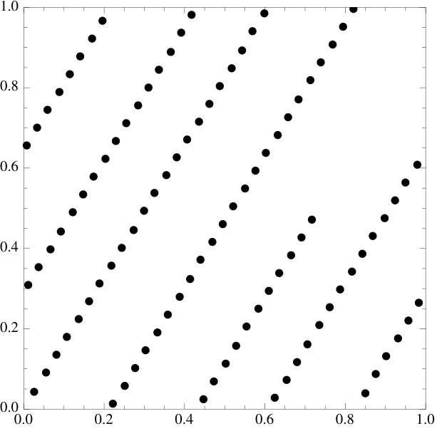 Figure 1
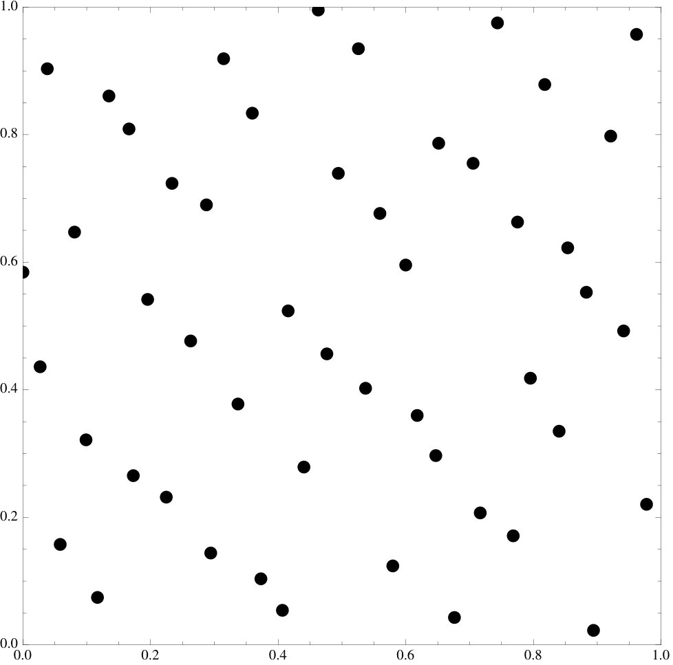 Figure 2
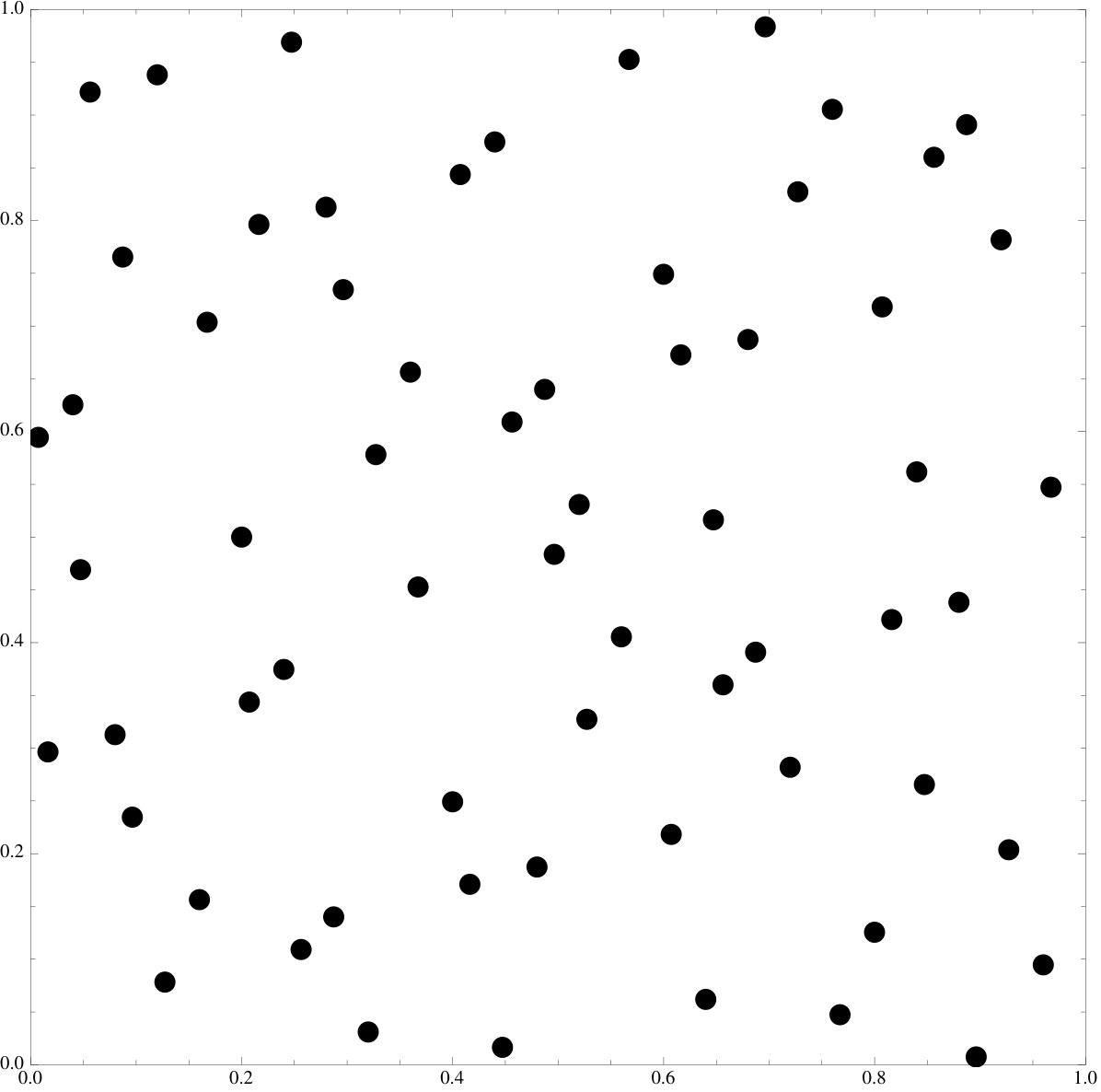 Figure 3
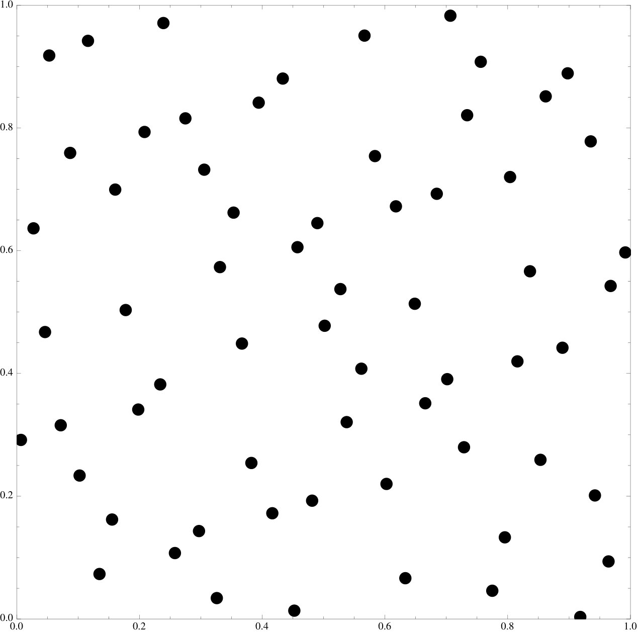 Figure 4
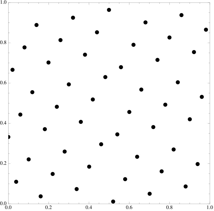 Figure 5
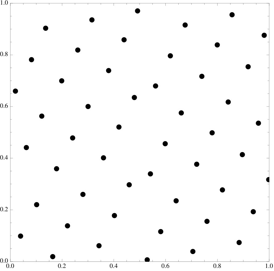 Figure 6
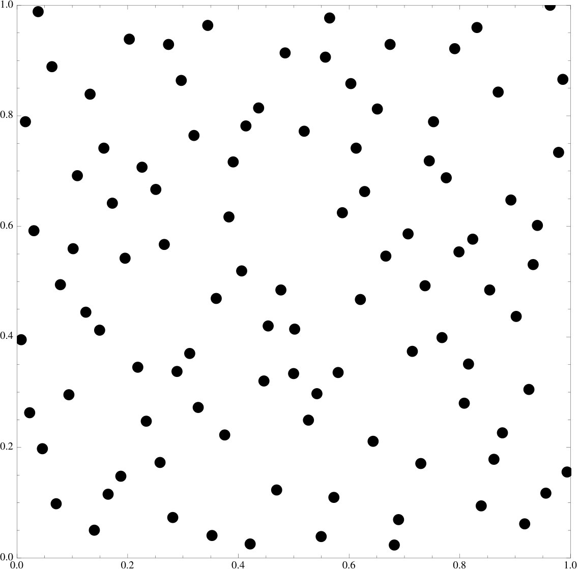 Figure 7
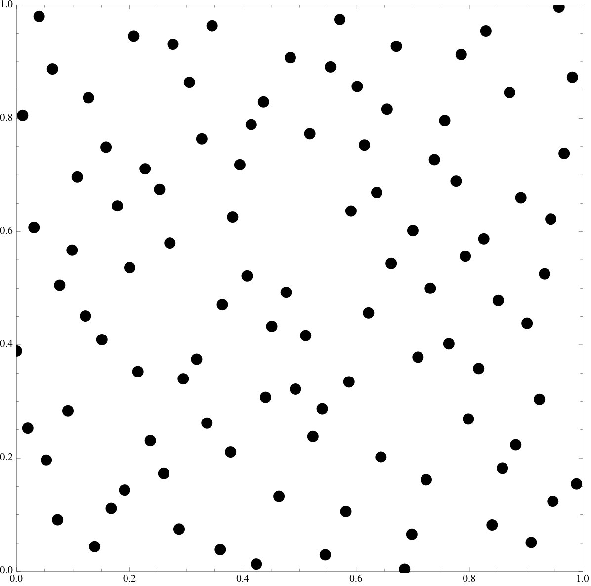 Figure 8
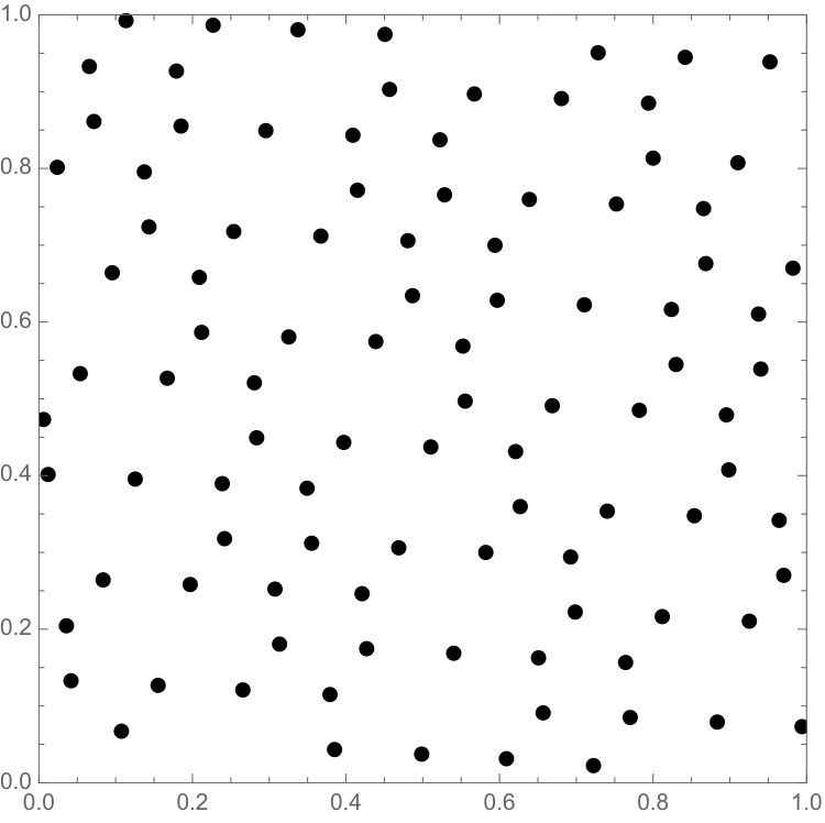 Figure 9
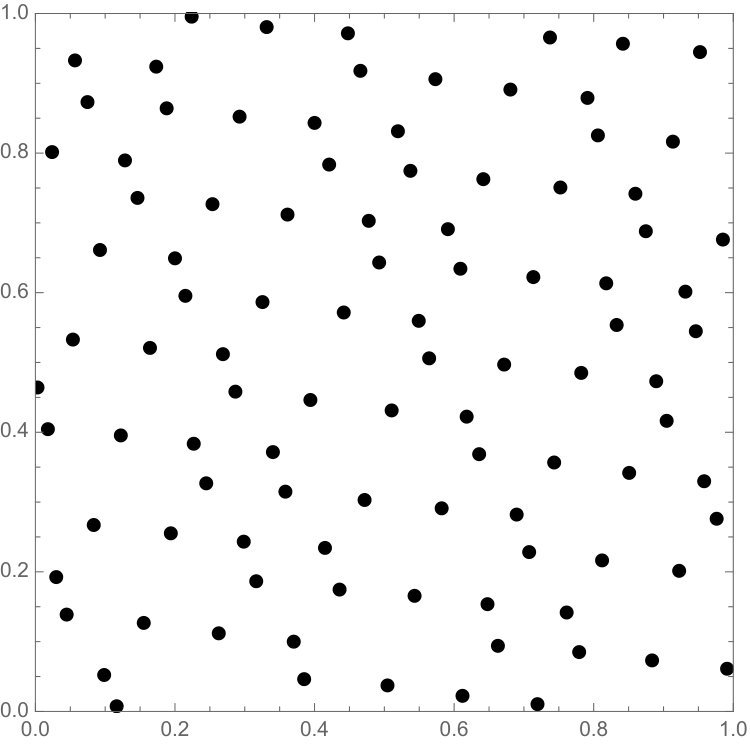 Figure 10
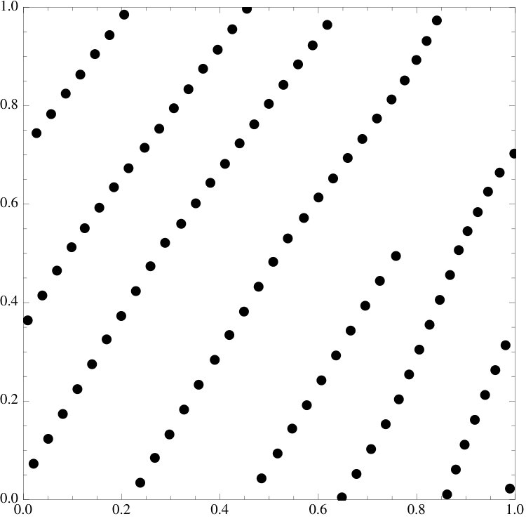 Figure 11
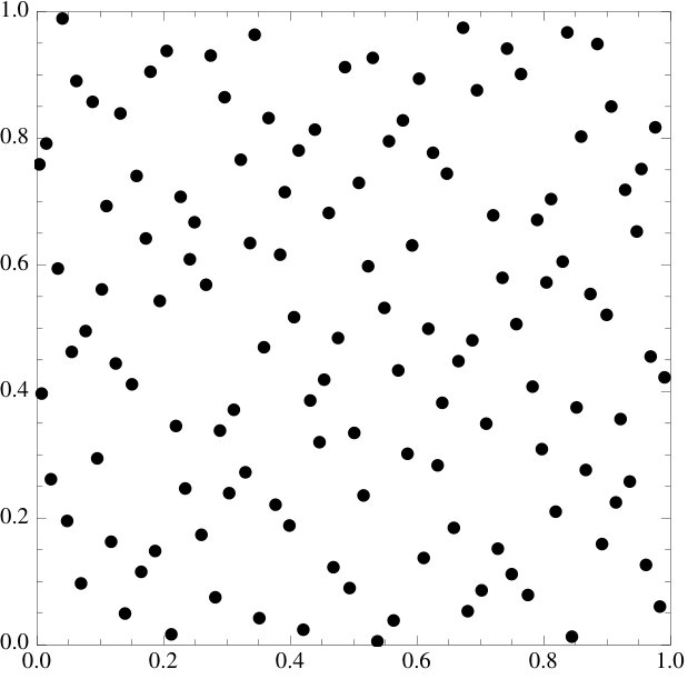 Figure 12
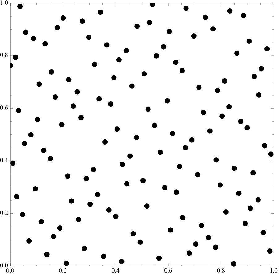 Figure 13
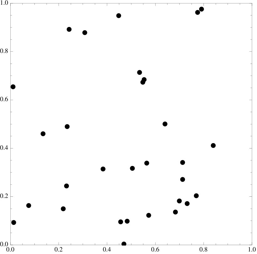 Figure 14
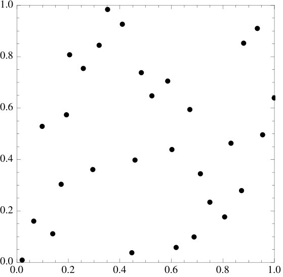 Figure 15
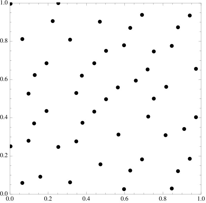 Figure 16
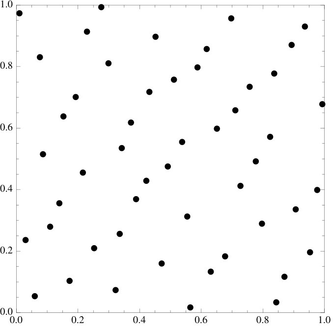 Figure 17
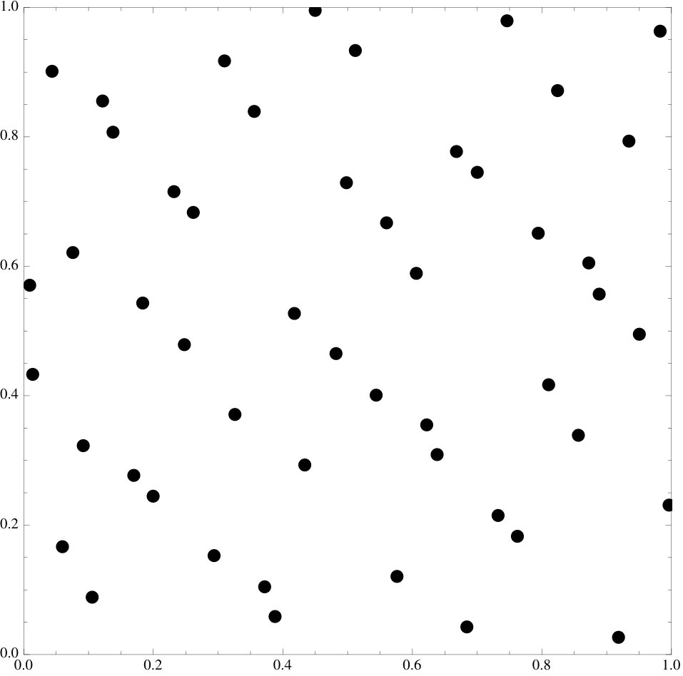 Figure 18
| Type of Sequences | Discrepancy | after Optimization | |
|---|---|---|---|
| Niederreiter sequence | 50 | 0.082 | 0.061 |
| Hammersley (base 3) | 50 | 0.064 | 0.042 |
| Sobol | 50 | 0.063 | 0.057 |
| Halton (base 2 and 5) | 64 | 0.064 | 0.045 |
| random points | 100 | 0.12 | 0.05 |
| Halton (base 2 and 3) | 128 | 0.032 | 0.025 |
| Niederreiter in | 50 | 0.098 | 0.093 |
| 100 | 0.074 | 0.066 |
Peer Reviews
No public reviews on file for this paper yet. If you reviewed it on a platform where reviews are public (OpenReview, ICLR, NeurIPS, ICML), you can paste yours below so the community can read it here.
Videos
No videos yet. Explain this paper in a talk, walkthrough, or lecture? Add one.
Taxonomy
TopicsMathematical Approximation and Integration · Cryptography and Residue Arithmetic
A Nonlocal Functional Promoting Low-Discrepancy Point Sets
Stefan Steinerberger
Department of Mathematics, Yale University, New Haven, CT 06511, USA
Abstract.
Let be a set of points in the dimensional torus that we want to arrange as regularly possible. The purpose of this paper is to introduce the energy functional
[TABLE]
and to suggest that moving a set into the direction may have the effect of increasing regularity of the set in the sense of decreasing discrepancy. We numerically demonstrate the effect for Halton, Hammersley, Kronecker, Niederreiter and Sobol sets. Lattices in are critical points of the energy functional, some (possibly all) are strict local minima.
Key words and phrases:
Low discrepancy sequence, gradient flow, energy functional.
2010 Mathematics Subject Classification:
11L03, 42B05, 82C22.
The author is supported by the NSF (DMS-1763179) and the Alfred P. Sloan Foundation.
1. Introduction
1.1. Introduction.
This paper is partially motivated by earlier results about how to distribute points on a manifold in a regular way. One idea (from [29, 35]) is to not construct these points a priori but instead use (local) minimizers of an energy functional. For example, suppose we want to distribute points on the two-dimensional torus in a way that is good for numerical integration. One way of doing this is by trying to find local minimizers of the energy functional
[TABLE]
where is a constant. These point configurations are empirically shown [29] to be better at integrating trigonometric polynomials than commonly used classical constructions, the reason for that being a connection between the Gaussian and the heat kernel (which, in itself, can be interpreted as a mollifier in Fourier space dampening high oscillation). This method is also geometry independent and works on general compact manifolds (with replaced by the geodesic distance).
1.2. The problem.
We were curious whether there is any way to proceed similarly in the problem of finding low-discrepancy sets of points. Suppose is a set of distinct points. A classical question is how would to arrange them so as to minimize the star discrepancy defined by
[TABLE]
A seminal result of Schmidt [32] is
[TABLE]
Many constructions of sets are known that attain this growth, we refer to the classical textbooks by Dick & Pillichshammer [6], Drmota & Tichy [12] and Kuipers & Niederreiter [23] for descriptions. Some of the classical configurations are also used as examples in this paper. The problem is famously unsolved in higher dimensions where the best known constructions [17, 18, 27, 28, 33] satisfy but no matching lower bound exists (see [3, 4, 5]). Indeed, there is not even consensus as to whether the best known constructions attain the optimal growth or whether there might be more effective constructions in .
We were interested in whether it is possible to assign a notion of ’energy’ to a set of points that vaguely corresponds to discrepancy in the sense that moving the points in such a way that perturbations of the points decreasing the energy also often decrease discrepancy. What would be of interest is a notion of energy that is
- (1)
fast to compute 2. (2)
often helpful in improving existing point sets 3. (3)
and may have the potential to lead to new constructions.
We believe this questions to be of some interest. The purpose of this paper is to derive one functional that seems to work very well in practice. Indeed, it works strikingly well: when applied to the classical low discrepancy constructions, it always seems to further decrease discrepancy (though sometimes, when the sets are already well distributed, only by very little). We provide a heuristic explanation in §3.3. There might be many other such functionals (possibly related to different kinds of mathematics, e.g. [2, 26, 30]) and we believe that constructing and understanding them could be quite interesting indeed.
Open Problem. Construct other energy functionals whose gradient flow has a beneficial effect on discrepancy. What can be rigorously proven? Can they be used for numerical integration? How do they scale in the dimension?
1.3. Related results.
We emphasize that this open problem stated in §1.2. is wide open. In particular, we do not claim that our energy functional is necessarily the most effective one. Our functional certainly seems natural in light of our derivation; moreover, the author recently used it [36] to define sequences whose discrepancy seems to be extremely good when compared to classical sequences (however, the only known bound for these sequences is currently ). Nonetheless, there may be other functionals that are as natural and even more efficient. As an example of another functional that could be of interest, we mention Warnock’s formula [24, Lemma 2.14] for the discrepancy
[TABLE]
This could be used to define a gradient flow (where one has to be a bit careful with the non-differentiability of the minimum). A similar construction is presumably possible at a much greater level by using integration formulas in reproducing kernel Hilbert spaces (see e.g. [7]). We recall that, if we sample in with weights , then the worst case error in a reproducing kernel Hilbert space is given by the formula
[TABLE]
Functionals of this flavor might be amenable to a gradient flow approach at a great level of generality, however, this is outside the scope of this paper.
To the best of our knowledge, the approach outlined in this paper as well as the associated functional is new. There is a broad literature around the underlying problem of construction of low-discrepancy sequences by various means. Traditional results where mainly concerned with asymptotic results (see e.g. [6, 12, 23]). These constructions often have implicit constants that grow very quickly in the dimension; the search for results that are effective for a small number of points initiated a fertile area of research [1, 10, 19, 20]. Even the mere task of computing discrepancy in high dimensions is nontrivial [11, 15, 16]. We are not aware of any optimization algorithms that take an explicit set of points and then induce a gradient flow to try to decrease the discrepancy.
1.4. Outline of the paper.
§2 introduces the energy functional and the main result. §3 explains how the energy functional was derived, describes the one-dimensional setting and relates it to Fourier analysis. A proof of the main result is given in §4. Numerical examples of how the energy functional acts on well-known constructions are given throughout the paper – these examples are all two-dimensional (for simplicity of exposition).
We emphasize that the examples of point sets are all essentially picked at random, the functional does seem to work at an overwhelming level of generality and we invite the reader to try it on their own favorite sets.
2. An energy functional
2.1. The functional.
Given a set of points in the dimensional torus where each point is given by
[TABLE]
we introduce the energy function via
[TABLE]
We note that, for we have that
[TABLE]
and so every term in the product is always positive. We also note that if two different points have the same th coordinate, then the functional is not defined and we set in that case. In practice, we can always perturb points ever so slightly to avoid that scenario. We note that the functional has an interesting structure: it very much likes to avoid having too many points that have very similar coordinates. This makes sense since such points can be easily captured by a thin (hyper-)rectangle. We now first discuss how to actually minimize it in practice and then discuss our main result.
2.2. How to compute things.
We are using the standard gradient descent: if is a differentiable function, gradient descent is trying to find a (local) minimum by defining an iterative sequence of points via
[TABLE]
were is the step-size. This is exactly how we proceed as well. The gradient can be computed explicitly and
[TABLE]
where
[TABLE]
This allows us to compute
[TABLE]
which is the infinitesimal direction in which we have to move to get the largest increase in the energy functional. Since we are interested in decreasing it, we replace
[TABLE]
The algorithm is somewhat sensitive to the choice of (this is not surprising and a recurring theme for gradient methods): it has to be chosen so small that the first order approximation is still somewhat valid, however, if it is chosen too small, then convergence becomes very slow and one needs more iterations to converge. In practice, for point sets containing points, we worked with which usually leads to a local minimum within less than a hundred iterations. The cost of computing a gradient step is of order when and thus not at all unreasonable. There are presumably ways of optimizing both the choice of as well as the cost of computing the energy (say, by fast multipole techniques) but this is beyond the scope of this paper.
2.3. Lattices.
We observe that if the initial point set is already very well distributed, then minimizing the energy tends to have very little effect on both the set and the discrepancy. There is one setting where this behavior is especially pronounced. We will consider lattice rules of the type
[TABLE]
where are coprime and is the fractional part. Lattice rules are classical examples of sequences with small discrepancy, we refer to [6, 12, 23] and refer to [8, 22] for examples of more recent results.
Theorem**.**
Every lattice rule is a critical point of the energy functional. Moreover, if , then is a strict local minimum.
We understand critical point in the following sense: if we fix all but one point and then move the one point distance , then the energy changes by a factor proportional to . If , then the energy changes like for some . Some restriction like this is clearly necessary since, if we move all the points by the same fixed vector, the energy remains unchanged. Nonetheless, we expect stronger statements to be true. We also do not know whether the condition is necessary, it seems like it should not be; we comment on this at the end of the paper. Several of the classical point sets (i.e. Sobol sequences) barely move under the gradient flow – is it maybe true that many classical sequences have a local minimum nearby?
2.4. Related functionals.
One question of obvious interest is whether there are related functionals. We point out that our functional is part of a natural 1-parameter family of functionals that are naturally defined via certain fractional integral operators. This is not how our functional was originally derived (that derivation can be found in §3 and is based on the Erdős-Turan inequality) but may provide an interesting avenue for further research. We note that our approach to the Erdős-Turan inequality involves an application of a Cauchy-Schwarz inequality that could also be done in a different fashion and this would, somewhat naturally, lead to the inverse fractional Laplacian. We quickly introduces this fascinating object here and then mention explicitly in the proof how one could deviate from the derivation. A full exploration of this case is outside the scope of this paper. If is sufficiently smooth, then we can differentiate term by term and obtain, for any ,
[TABLE]
However, as is easily seen, this definition actually makes sense for : if is positive, then we require that decays sufficiently quickly for the sum to be defined. If is negative, then it suffices to assume that since for all (we refer to [31] for an introduction into the fractional Laplacian on the Torus). We will now compute , where is a Dirac measure in 0 in . We see that
[TABLE]
This is, up to a factor of , exactly the factor arising in our computation. It is well understood that is a special scale and that the fractional Laplacian has different behavior for and but it does suggest many other factors that can be computed in a similar way. It also suggests that it might be potentially worthwhile to study functionals of the type
[TABLE]
which can be simplified
[TABLE]
Using self-adjointness of the inverse fractional Laplacian, we can simplify the relevant term as
[TABLE]
This, in turn, can be rewritten as
[TABLE]
which, obviously, admits a gradient formulation. One could also consider a possible trunction in frequency followed by a gradient formulation as well as various mollification mechanism. We want to strongly suggest the possibility that the optimal value of for these kinds of methods may depend on the dimension.
3. Heuristic Derivation of the Energy Functional
We first give a one-dimensional argument to avoid notational overload and then derive the analogous quantity for higher dimensions in §3.2.
3.1. One dimension.
Our derivation is motivated by the Erdős-Turan inequality bounding the discrepancy of a set by
[TABLE]
We can bound this from above, using valid for all real , by
[TABLE]
Using merely this upper bound, we want to make sure that the second term is small. This second term simplifies to
[TABLE]
Ignoring the scaling factor , we decouple into diagonal and off-diagonal terms and obtain
[TABLE]
The first term is a fixed constant and thus independent of the actual points, the second sum can be written as
[TABLE]
The inner sum can now be simplified [25] by letting the limit go to infinity since
[TABLE]
This suggests that we should really try to minimize the functional
[TABLE]
Remark. There is one step in the derivation where we could have argued somewhat differently: we could have written, for any ,
[TABLE]
The first sum simplifies to either to (for ), to (for ) or to (for ). The second term simplifies, after squaring the inner term and taking the limit of over the Fourier series, to the definition of the fractional Laplacian (see §2.4.) applied to the measure .
3.2. Higher dimensions.
The general case follows from the Erdős-Turan-Koksma [13, 14, 21] inequality and the heuristic outlined above for the one-dimensional case. We recall that the Erdős-Turan-Koksma inequality allows us to bound the discrepancy of a set by
[TABLE]
where is given by
[TABLE]
We note that, since , we can change to at merely the cost of a constant depending only on the dimension and thus
[TABLE]
The second sum we can expand into
[TABLE]
Letting , we can simplify every one of these terms to
[TABLE]
and we obtain the general form of the energy functional.
The Erdős-Turan-Koksma inequality shows
[TABLE]
We know that the best possible behavior is on the scale of (or possibly even smaller). This suggests that the exponential sums cannot typically be that large, it should be roughly at scale most of the time. Understanding this better could lead to precise estimates comparing how much our energy exceeds the discrepancy. We conclude by establishing a rigorous bound.
Lemma**.**
We have, for ,
[TABLE]
Proof.
The argument outlined above already establishes the result except for one missing ingredient: for all , there is a uniform bound
[TABLE]
We can assume w.l.o.g. that . We use Abel summation to write
[TABLE]
The first term is , it remains to treat the integral. The first term has the structure of an alternating Leibniz series with the first root being at . Thus
[TABLE]
The second integral simplifies to
[TABLE]
∎
3.3. The case .
Things are usually simpler in one dimension (though also less interesting because the optimal constructions are trivial and given by equispaced points). We have the following basic result.
Proposition**.**
Let be a sequence in . If
[TABLE]
then the sequence is uniformly distributed.
Proof.
The proof is similar in spirit to the main argument in [34], we refer to that paper for definition of the Jacobi function and the main idea. We define a one-parameter family of functions via
[TABLE]
where is the Jacobi function. In particular
[TABLE]
Defining
[TABLE]
we can define the function
[TABLE]
is monotonically decaying in time. This is seen by applying the Plancherel theorem
[TABLE]
and using . We can now take the limit and obtain that
[TABLE]
As for the second part of the argument, suppose that is not uniformly distributed. Weyl’s theorem implies that there exist such that
[TABLE]
Then, however,
[TABLE]
for some and infinitely many . ∎
4. Proof of the Theorem
4.1. An Inequality.
We first prove an elementary inequality.
Lemma**.**
Let . Then
[TABLE]
Proof.
The right-hand side is always positive, we can thus assume w.l.o.g. that . Multiplying with on both sides leads to the equivalent statement , where
[TABLE]
and
[TABLE]
We use to argue that
[TABLE]
The result then follows from the inequality
[TABLE]
which can be easily seen by elementary methods. ∎
4.2. Proof of the Theorem
Proof of the Theorem..
The symmetries of the sequence and the energy functional imply that it is sufficient to show that the energy is locally convex around the point in . This means we want to show that
[TABLE]
is strictly positive for all sufficiently small. We can assume , expand the first term in up to second order and note that
[TABLE]
This shows that
[TABLE]
We group the summand and and observe that is odd on while the second summand is even, therefore the sum evaluates to 0. The other derivative
[TABLE]
vanishes for exactly the same reason and therefore the lattice is a critical point. It remains to show that it is a local minimizer which requires an expansion up to second order. This expansion naturally decouples into three sums, where
[TABLE]
We can now argue that is bounded by
[TABLE]
The Lemma implies that we can bound the first term by
[TABLE]
We finally use the algebraic structure and argue that if , then
[TABLE]
and that implies that both sums are actually the same sum written in a different order. The arising sum is actually the term we are given in . The argument for the third sum is identical and altogether we conclude that
[TABLE]
which implies the desired result. ∎
It remains an open question whether the same result remains true in general. Basic numerical experiments suggest that this should be the case. We can reformulate the problem by writing out the quadratic form and computing its determinant. The relevant question is then whether where
[TABLE]
The reference list from the paper itself. Each links out to its DOI / PubMed record.
- 1[1] C. Aistleitner, Covering numbers, dyadic chaining and discrepancy, Journal of Complexity 27(6), p. 531-540, 2011.
- 2[2] A. Baernstein II, A minimum problem for heat kernels of flat tori. Extremal Riemann surfaces (San Francisco, CA, 1995), 227–243, Contemp. Math., 201, Amer. Math. Soc., Providence, RI, 1997.
- 3[3] D. Bilyk, Roth’s orthogonal function method in discrepancy theory, Uniform Distribution Theory 6 (2011), no. 1, 143–184.
- 4[4] D. Bilyk and M. Lacey, On the small ball Inequality in three dimensions, Duke Math. J. 143 (2008), no. 1, 81–115.
- 5[5] D. Bilyk, M. Lacey and A. Vagharshakyan, On the small ball inequality in all dimensions, J. Funct. Anal. 254 (2008), no. 9, 2470–2502.
- 6[6] J. Dick and F. Pillichshammer, Digital Nets and Sequences. Discrepancy theory and quasi-Monte Carlo integration. Cambridge University Press, Cambridge, 2010.
- 7[7] J. Dick and F. Pillichshammer, Discrepancy Theory and Quasi-Monte Carlo Integration, in: A Panorama of Discrepancy Theory, Springer, 2014.
- 8[8] J. Dick, D. Nuyens, F. Pillichshammer, Lattice rules for nonperiodic smooth integrands, Numerische Mathematik 126, p. 259-291, 2014