Trigonometric series and self-similar sets
Jialun Li, Tuomas Sahlsten

TL;DR
This paper demonstrates that certain self-similar sets in one dimension are sets of multiplicity, meaning trigonometric series are not unique outside these sets, by showing associated measures have Fourier transforms tending to zero.
Contribution
It proves that self-similar sets with irrational log-ratio contractions are sets of multiplicity, establishing Fourier decay for measures on these sets without separation conditions.
Findings
Self-similar sets with irrational log ratios are sets of multiplicity.
Self-similar measures on these sets are Rajchman measures.
Fourier transform decay rate is logarithmic under diophantine conditions.
Abstract
Let be a self-similar set on associated to contractions , , for some finite , such that is not a singleton. We prove that if is irrational for some , then is a set of multiplicity, that is, trigonometric series are not in general unique in the complement of . No separation conditions are assumed on . We establish our result by showing that every self-similar measure on is a Rajchman measure: the Fourier transform as . The rate of is also shown to be logarithmic if is diophantine for some . The proof is based on quantitative renewal theorems for stopping times of random walks on .
Click any figure to enlarge with its caption.
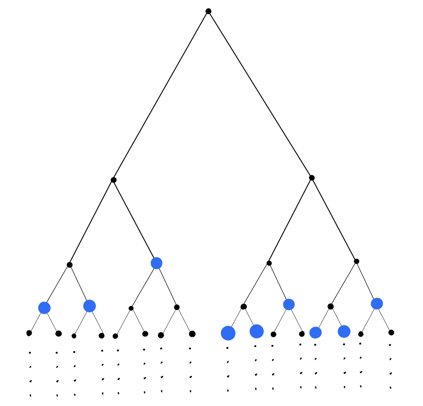 Figure 1
Peer Reviews
No public reviews on file for this paper yet. If you reviewed it on a platform where reviews are public (OpenReview, ICLR, NeurIPS, ICML), you can paste yours below so the community can read it here.
Videos
No videos yet. Explain this paper in a talk, walkthrough, or lecture? Add one.
Trigonometric series and self-similar sets
Jialun Li
Institut de Mathématiques de Bordeaux, Université de Bordeaux, 351 cours de la Libération, Talence, France
Current address: Institut für Mathematik, Universität Zürich, 190 Winterthurerstrasse, Zürich, Switzerland
and
Tuomas Sahlsten
School of Mathematics, Alan Turing Building, University of Manchester, Oxford Road, Manchester, UK
Abstract.
Let be a self-similar set on associated to contractions , , for some finite , such that is not a singleton. We prove that if is irrational for some , then is a set of multiplicity, that is, trigonometric series are not in general unique in the complement of . No separation conditions are assumed on . We establish our result by showing that every self-similar measure on is a Rajchman measure: the Fourier transform as . The rate of is also shown to be logarithmic if is diophantine for some . The proof is based on quantitative renewal theorems for stopping times of random walks on .
Key words and phrases:
Fourier analysis, Trigonometric series, Fourier series, self-similar sets, random walk on groups, renewal theory, metric number theory
2010 Mathematics Subject Classification:
42A20 (Primary), 42A38, 37C45, 28A80, 60K05 (Secondary)
TS was partially supported by the Marie Skłodowska-Curie Individual Fellowship grant 655310 and a start-up fund from the School of Mathematics, University of Manchester, UK
1. Introduction and the main result
The uniqueness problem in Fourier analysis that goes back to Riemann [42] and Cantor [10] concerns the following question: suppose we have two converging trigonometric series and with coefficients such that for “many” they agree:
[TABLE]
then are the coefficients for all ? For how “many” do we need to have (1.1) so that holds for all ? If we assume (1.1) holds for all , then using Toeplitz operators Cantor [10] proved that indeed for all . However, it would be interesting to see how small the set of satisfying (1.1) can be, so that we have for all . Motivated by this one defines that a subset is a set of uniqueness if whenever we have coefficients , , such that (1.1) holds for all , then for all . Here one defines also that if is not a set of uniqueness, then it is called a set of multiplicity. In particular by Cantor’s result this shows that the empty set is a set of uniqueness and so is a set of multiplicity.
Cantor [10] proved that that every closed countable set is a set of uniqueness, and later Young [56] generalised to every countable set. In the uncountable case, however, even if assuming is very small, uniqueness of may fail: Menshov [39] constructed a set of Lebesgue measure [math], which is a set of multiplicity, that is, the uniqueness problem fails if we only assume (1.1) for all . This can be proved using the following criteria, which goes back to Salem [44] that if a set supports a Borel probability measure such that the Fourier transform
[TABLE]
satisfies as , , then is a set of multiplicity. Such measures are called Rajchman measures in the literature. Hence constructing measures with decaying Fourier coefficients provides a way to check whether is of multiplicity. It remains an open problem to classify which uncountable sets are of multiplicity and which are of uniqueness and much work has been done in many examples of on trying to establish their uniqueness or multiplicity, see for example the works of Kechris et al. [32] on connections to descriptive set theory.
In the series of works Salem [44] proved that the middle third Cantor set is a set of uniqueness. More generally, Salem established that if is the middle -Cantor set with , that is, interval of length is removed from the center of at every construction stage, then is a set of uniqueness when is a Pisot number. In the opposite case, if is not a Pisot number, by constructing a Rajchman measure on , Piatetski-Shapiro [40], Salem and Zygmund [45] established that is a set of multiplicity.
The Cantor set is an example of a self-similar set. Recall that a subset is self-similar if there exists similitudes , that is, , , for some finite set , translations and contractions such that
[TABLE]
As far as we know nothing is known about the uniqueness or multiplicity of self-similar sets beyond the case of or if adding finitely many more similitudes with the same contraction ratio to the definition, which was done by Salem [44]. For example if we have two different contractions and for the iterated function system, do we expect to be of multiplicity or of uniqueness? Due to having same contraction ratio the case has a convolution structure, which is helpful when connecting to the algebraic properties of the number . In the general case, however, we would need to find a way out of this.
It turns out that the algebraic properties of the additive subgroup generated by the log-contraction ratios in is important in the study of the multiplicity of a self-similar set with contraction ratios . In particular if this subgroup is dense, which happens when is irrational for some (e.g. and ), we can establish is a set of multiplicity.
Theorem 1.1**.**
Let be a self-similar set associated to contractions , , such that is not a singleton. If is irrational for some , then is a set of multiplicity.
Notice that by assuming is irrational we exclude the case of as in that case every ratio of logarithms of the contractions is just . It remains an open problem to study the case when for all . We predict that here typically should be a set of uniqueness unless all the contraction ratios are equal, like the case , and then an algebraic number theoretic condition like being Pisot needs to be imposed.
In order to prove the multiplicity of a self-similar set , it is enough by Salem’s criterion [44] for multiplicity to find a Rajchman measure supported on . Hence Theorem 1.1 follows by establishing that all positive dimensional self-similar measures on are Rajchman measures. Recall that a probability measure on is called self-similar if there exists a finite collection of similitudes of with at least two maps and weights , , with such that .
Theorem 1.2**.**
Let be a self-similar set associated to contractions , , such that is not a singleton. If is irrational for some , then the Fourier transform as for every self-similar measure on .
Theorem 1.2 is closely related to another currently active problem in the community of fractal geometry, where we would like to understand the Fourier transforms of fractal measures, see the book [38] by Mattila for an history and overview. In particular there are various past and recent works on random fractals by Kahane [26, 27], Shmerkin and Suomala [48] and other people [19, 20], connections to Diophantine approximation by Kaufman et al. [28, 29], dynamical systems [24, 43] and additive combinatorics [4, 33]. Analysing the spectrum of fractal measures has been particularly important in finding normal numbers from the support of fractals [23, 41, 14] and the study of harmonic analysis defined by fractal measures, see for example applications to the spectrum of convolution operators defined by fractal measures in the work of Sarnak [46] and later by Sidorov and Solomyak [50], and more recently applications to quantum resonances in quantum chaos by Bourgain and Dyatlov [5].
The study of Fourier transforms of self-similar measures in general goes back to the works of Strichartz [51, 52], where an average decay of Fourier transform of self-similar measures was obtained, where proportions of frequencies are excluded. More recently a large deviation estimate for these average decays was proved by Tsujii [53]. However, the methods here cannot be used to obtain a full decay over all . Before Theorem 1.2 the only cases of self-similar measures where as was known were Bernoulli convolutions , , which are the distribution of the random sum with i.i.d. chosen signs. The case was studied by Piatetski-Shapiro [40], Salem and Zygmund [45], where up to a translation are natural self-similar measures on middle Cantor set. For Bernoulli convolutions with Fourier transforms play an important role. In particular, proving that has sufficiently fast power decay as implies that is absolutely continuous, which is a well-known open problem in the field, see for example Shmerkin [47]. It is known by the results of Erdös [21] and Kahane [25] that the set of such that does not have a power decay has Hausdorff dimension zero. Moreover, if is is not a Pisot number, then Salem [44] proved as , and conversely if is a Pisot number, Erdös [21] proved that as . In the non-Pisot case the rate of convergence was later shown to be logarithmic for rational number by Kershner [31], see also Dai [12] and Bufetov and Solomyak [9], and some power decay for algebraic numbers has been obtained by Dai, Feng and Wang [13].
Notice that in Theorem 1.1 and Theorem 1.2 there can be any types of overlaps for the maps and no separation conditions are assumed. Typically in the overlapping case the analysis of self-similar sets and measures can be notoriously difficult to understand, say, their Hausdorff dimension has required some deep connections to additive combinatorics, see for example the recent works of Hochman [22], Breuillard-Varjú [8] and Varjú [54]. The reason overlaps do not cause us any issues is the fact that the main contribution to the Fourier decay comes from controlling the distribution of lengths of the construction intervals, and not their relative positions. Understanding the distribution of the lengths of the construction intervals then can be reduced as a problem of studying the renewal theory for stopping times of random variables on with distribution . This strategy to establish Fourier decay is inspired by the case of the stationary measure for Lie group actions by the first author in [35]. In the self-similar case case we consider, however, the proof is much more straightforward and we can see the idea governing the Fourier decay more clearly. In our case we will prove a quantitative version of Kesten’s renewal theorem for stopping time given in [30], see Section 2. The irrationality of is key to prove the random walk becomes non-lattice, that is, not concentrated on an arithmetic progression, which is a key assumption for the renewal theorem for stopping times we employ.
If we want a rate of convergence in Theorem 1.2 using the strategy we present in this paper, one needs to go into the rate of convergence for the renewal theorems we use. Here it is well-known that the diophantine properties of the random walk become an essential property, in particular, how well is approximated by rationals. In Diophantine approximation, it is defined that an irrational real number is called diophantine if for some and we have
[TABLE]
for all and . This happens for example when or in general for with coprime, see Baker [1]. Having some diophantine in the iterated function system imposes the random walk generated by the contractions to quantitatively avoid lattices and then gives quantitative rates for the renewal theorem. Under this condition, we can improve Theorem 1.2 in the following way:
Theorem 1.3**.**
Let be a self-similar set associated to contractions , , such that is not a singleton. If is diophantine for some , then for every self-similar measure on , there exists such that
[TABLE]
Remark 1.1*.*
By using a quantitative equidistribution criterion by Davenport-Erdös-LeVeque [14], a particular consequence of the logarithmic decay for Fourier transform of a probability measure on is that almost every number is normal in every base. Thus in the setting of Theorem 1.3 we have for any self-similar measure on that almost every number is normal in every base. This consequence was pointed out in [18] and we thank Mel Levin for bringing this to our attention.
Removing the irrationality of ratios of log-contractions ratios makes the random walk on generated by a lattice, that is, concentrated on an arithmetic progression. Then the renewal theorems do not hold anymore in the same form. In fact, for example in the case of middle Cantor measure, the Fourier transform does not even decay at infinity. However, in the case is not Pisot, the Bernoulli convolution associated to provides examples of a measure where the Fourier transform does decay at infinity, even with polynomial rate for some algebraic , but the additive random walk on generated by is a lattice. Hence it would be interesting to develop the connection to renewal theory further and find a full classification of self-similar sets which are of uniqueness and which are of multiplicity. After the completion of this manuscript, these problems have been addressed by Brémont [7] and Varjú-Yu [55]. Moreover, the polynomial Fourier decay case was recently obtained for most self-similar measures by Solomyak [49].
In this paper we consider the self-similar case, but if we impose that the maps to be suitably nonlinear, such as the inverse branches of the Gauss map and study the Fourier transforms of self-conformal measures , then the rates of Fourier decay in Theorem 1.3 for Fourier decay can be improved to power decay, see for example the works [24, 5, 43, 36]. Here the non-lattice condition of contractions is replaced by a non-concentration condition of the log-derivatives of the iterates as . These types of conditions appear in the Fourier decay properties of multiplicative convolutions in the discretized sum-product theory developed by Bourgain [4].
What about the higher dimensional case? Here the analogue to Theorem 1.2 and Theorem 1.3 would be to understand Fourier transforms of self-affine measures on . They are measures on associated to affine contractions of , , for some finite set , where and such that
[TABLE]
for some weights , , with . In a follow-up paper [37], we apply a similar strategy as we do in this paper by considering renewal theory for random walks on the group coming from to establish a Fourier decay for self-affine measures. The renewal theory we need has been done recently by the first author in [36]. Here the non-lattice condition can be replaced by an irreducibility and proximality assumption of the subgroup generated by as Bárány, Hochman and Rapaport did recently in their work [2] for the computation of Hausdorff dimension of self-affine measures on . Moreover, due to the better rates for quantitative renewal theorems for random walks in real split groups [36], that is, when the Zariski closure of is -splitting, we can improve the rates for the Fourier decay of to power decay.
Organisation of the paper. The article is organised as follows. In Section 2 we describe the key method used in the paper and give the quantitative renewal theorems we need for our results and then prove them in Section 4. Then in Section 3 we give the proof of Theorem 1.2, which implies Theorem 1.1 on the multiplicity of self-similar sets, and also in Section 3 we prove the quantitative Theorem 1.3 using the quantitative estimates for the renewal theorem stated in Section 2.
2. Renewal theorems for stopping time of random walks in
The main method used to establish Theorems 1.2 and 1.3 is based on renewal theory. Renewal theory has a long history of research both in probability theory and dynamical systems, see e.g. [17, 34] and various other works citing them. Here we will need quantitative renewal theorems for stopping time of random walks in , which we will now describe.
Suppose is a probability measure on with finite support. Let
[TABLE]
be the expectation of , which is positive by definition. Renewal type results are valid under more general assumption. For simplicity, we state it under this simple assumption which is sufficient for the proof of main results in the manuscript. Let be i.i.d. sequence of random variables in with probability distribution . Write for the sum
[TABLE]
For a non-negative bounded Borel function on , define the renewal operator by
[TABLE]
Because of the non-negativity of , this sum is well defined. Kesten’s key renewal theorem [30] considers the limit behaviour of as . The algebraic properties of the support of the distribution will be crucial in the behaviour of as . If is non-lattice, that is, generates a dense additive subgroup of , then the limit as is given by , where is the Lebesgue measure.
Here we need to study the convergence for randomly stopped processes at a stopping time
[TABLE]
and see how the residual process behaves as . Kesten’s renewal theorem for stopping time [30] says that the residue distribution will converge to a distribution absolutely continuous with respect to the Lebesgue measure when tends to infinity.
Let be the supremum of the absolute value of the elements in the support of . Define a local norm on the interval by
[TABLE]
We will have the following renewal theorem.
Proposition 2.1**.**
If is a probability measure on with finite support and non-lattice, then we have for and a function on the following asymptotics as :
[TABLE]
where tends to zero as is going to . Here is a piecewise constant function and vanishes when passes the support of .
Proposition 2.1 is equivalent to the classical Kesten’s renewal theorem for stopping time [30]. Because the unit ball of is precompact in , the uniform speed on norm is equivalent to the convergence in distribution of , which is exactly Kesten’s theorem. We thank one of the anonymous referees for pointing this out to us.
Proposition 2.1 will be used to prove Theorem 1.2 later in Section 3 and the non-lattice condition for is obtained using the irrationality of . However, in the setting of Theorem 1.3, where we assume is diophantine, we will need a quantitative version of Proposition 2.1, where one needs a stronger assumption on the distribution called (-)weakly diophantine, that is, for some :
[TABLE]
where is the Laplace transform of , defined for by the formula
[TABLE]
This condition means heuristically that the random walk quantitatively avoids concentration on lattices and could be considered as a spectral gap condition for the random walk. The number will be reflected in the rate of the renewal theorem for stopping time of random walks:
Proposition 2.2**.**
If is -weakly diophantine, then for we have
[TABLE]
This polynomial error term is new for the renewal theorem for stopping time. A polynomial error term in the key renewal theorem was obtained by Carlsson in [11] under the same weakly diophantine hypothesis using Fourier transform. What we do here uses key renewal theorem to prove renewal theorem for stopping time and we track the error term carefully such that the error term in renewal theorem for stopping time can be computed using error term in key renewal theorem. With stronger hypothesis, that is , Blanchet and Glynn give an exponential error term of key renewal theorem in [3]. However, this stronger hypothesis is never true for finitely supported measures . See [6] for more details and bibliography on the error term of the key renewal theorem.
In our case of self-similar measures associated to an iterated function system and weights , the random walk we will use is given by , , where with probability . Thus In Section 3 we verify the assumptions of the renewal theorems Proposition 2.1 and Proposition 2.2. We will explain how they are used to prove the main results on Fourier decay.
3. Proof of the Fourier decay
3.1. Symbolic notations
Let us write as the space of all words with entries in of finite length. Moreover, is the space of all words of length with entries in and the infinite length words. If , define the composition
[TABLE]
Then is again a similitude with a contraction
[TABLE]
Using this notation the self-similarity of implies that
[TABLE]
where
[TABLE]
as the product of weights , , according to the entries of the word . See the book by Falconer [15] for more details, notations and history on self-similar sets and measures.
3.2. Reduction to exponential sums
Given and , the first step is to reduce the Fourier transform of to double integrals over exponential sums determined by a stopping time . Recall that we defined in Section 2 for the stopping time
[TABLE]
where and are i.i.d. random variables distributed according to
[TABLE]
We can identify the stopping time as follows using symbolic notations. For an infinite word write as the smallest such that the restriction satisfies , that is . Thus in particular will be roughly : we have for some constant . Then this symbolic definition agrees with the stopping time by setting the probability space with , is the Borel -algebra generated by cylinder sets and . With this in mind, write
[TABLE]
and let be the probability distribution on associated to the stopping time, that is,
[TABLE]
Thus the support . Now the distribution of agrees with the distribution of , where follows the distribution of . Then for a continuous function on we obtain
[TABLE]
See Figure 1 for an illustration of the words .
The reason to use the stopping time here is that we want to use the equidistribution phenomenon of the renewal theorem (Proposition 2.1), which combined with high-oscillation can give decay of exponential sums.
Later we will make depend on and let , but for now we keep everything fixed.
Lemma 3.1**.**
For every and we have
[TABLE]
Proof.
Firstly, by
[TABLE]
and the martingale stopping theorem, we see that for any , we can write
[TABLE]
(The proof of this is similar to [35, Proposition 3.5].) Hence we obtain
[TABLE]
Thus by Cauchy-Schwarz, we have
[TABLE]
Opening up we see that
[TABLE]
∎
Thus to prove Fourier decay, we would need to prove
[TABLE]
as for a suitable . If we want a rate for the Fourier decay, we need to control the speed of convergence in (3.2). In order to do this, we first write as follows
[TABLE]
using parameters and . Later we will first take large, then take large enough depending on . Using these parameters, write
[TABLE]
Then define the tube in :
[TABLE]
We will split (3.2) into two cases depending on how close and are in terms of the defined above. We will have the following two propositions given in Proposition 3.2 and Proposition 3.3, which together imply Theorem 1.2. For the quantitative part, we also need Proposition 3.5 to control the rate in (3.2).
3.3. Controlling nearby points
The first one is on the nearby points , that is, those with , and here is where we use the fact that is not a singleton. By [16, Proposition 2.2], due to is not a singleton, there exist , and such that for all and we have
[TABLE]
A measure which satisfies this condition is sometimes called Hölder regular. Using the decay (3.4) of the measure on balls, we can control the nearby points in the following lemma:
Proposition 3.2**.**
There exists such that for any , where is chosen such that the condition (3.4) hold for , and for all , we have
[TABLE]
Proof.
First of all, since for all we have that
[TABLE]
Thus we can bound using the triangle inequality as follows
[TABLE]
since for all . Using Fubini’s theorem we see that
[TABLE]
thus by (3.4) the right-hand side is bounded by a constant multiple of . ∎
3.4. Application of the renewal theorem and high-oscillations
In the case when are chosen such that , we will use the renewal theory to prove the following convergence:
Proposition 3.3**.**
Suppose is irrational for some . If and , then
[TABLE]
The proof of Proposition 3.3 follows from the renewal theorem for stopping time of random walks (Proposition 2.1). The rate in Proposition 3.3 is not quantitative. In the later section, by adding an extra assumption ( is diophantine) to the renewal theory, we can apply the quantitative version (Proposition 3.5).
Proof of Proposition 3.3.
By definition of we have that for all and the difference
[TABLE]
Therefore we can write
[TABLE]
Recall that we have fixed and such that has the form . With this , we can define a smooth function by
[TABLE]
Then the local norm of satisfies , as , recall (2.1) for the definition of local norm. Using and (3.1) we can write for any pair that
[TABLE]
Due to the irrationality of for some , the additive subgroup generated by , , is dense in . So is non-lattice and we can apply Proposition 2.1. We apply Proposition 2.1 with the function , which gives us for that
[TABLE]
If we now look at the right-hand side, since is a piecewise continuous function, or just integrable, Riemann-Lebesgue lemma implies that for all we have
[TABLE]
However, to be able to use the above convergence (3.7), we need uniformity in terms of and in this convergence and to make it more effective using the error term in the renewal theorem Proposition 2.1.
Recall that in (3.3) we defined depending on as and . Thus if and , we have
[TABLE]
where is the diameter of .
Therefore, by (3.6) and applying Proposition 2.1
[TABLE]
where we can take the limit because the error term
[TABLE]
is uniform for by (3.8). The proof is complete by (3.7).
∎
Proposition 3.3 together with Proposition 3.2 and Lemma 3.1 completes the proof of Theorem 1.2 as follows:
Proof of Theorem 1.2.
By Proposition 3.2, we have for all large enough with and for all that:
[TABLE]
where , and is a universal constant. Thus
[TABLE]
On the other hand, Proposition 3.3 implies that we have
[TABLE]
Hence Lemma 3.1 gives
[TABLE]
which gives the claim. ∎
3.5. Quantitative rate for Fourier decay
In order to prove a quantitative rate (Theorem 1.3), we need a rate in Proposition 3.3. For this purpose we will employ Proposition 2.2. So we need to verify weakly diophantine condition for , which will follow from the diophantine assumption in Theorem 1.3. From now on, we use a notation to mean there exists a universal constant such that , and for that respectively.
Lemma 3.4**.**
If there exist for such that is diophantine, then the measure is weakly diophantine.
Proof.
Indeed, we have
[TABLE]
with . By the definition (1.2) of a diophantine number, we obtain that for some
[TABLE]
which implies is weakly diophantine. ∎
Now we can prove the following quantitative version of Proposition 3.3, which implies Theorem 1.3:
Proposition 3.5**.**
Suppose is diophantine for some . Then there exists such that
[TABLE]
as , where satisfies .
Proof.
Since is weakly diophantine by Lemma 3.4, we can apply Proposition 2.2 to obtain for some that for :
[TABLE]
Because the function , , is piecewise constant with a finite number of points of discontinuity, the decay rate in the main term, the oscillation integral, is given by the oscillation (See [35, Lemma 3.8] for more details)
[TABLE]
Then we take , which implies for for equal to the diameter of the support of . When , we have, after taking logarithms that the rate is given by , which gives the claim. ∎
4. Proofs of the renewal theorems
In this section we will prove Proposition 2.1 and 2.2. They follow the similar proofs for the stationary measure for Lie group actions in [35], but here we will give a full self-contained proof in order to present the method in the most basic setting. Let us now give a brief overview of the proofs presented here. First of all, we will give a proof of key renewal theorem for good functions using Laplace transform in Proposition 4.2, with a control of error term. Then in order to find the limit of the distribution of the process , we will consider the joint distribution of and prove a renewal theorem for this joint distribution in Proposition 4.7 using Proposition 4.2. Then we add the cutoff assumption that and . In Proposition 4.10 we prove a renewal theorem for the joint distribution of under this cutoff assumption. Finally, the reason we are doing this is that the distribution of is exactly the sum over natural numbers of the distribution of the sum under the cutoff assumption of .
In the following sections we actually only need that is supported on , non-lattice, and has an exponential moment: there exists such that
[TABLE]
The exponential moment assumption is more general than the finite support hypothesis of in Section 2. However, in the proofs of Propositions 2.1 and 2.2 we will impose that has a finite support, see Section 4.6 for their proofs. With a bit more effort, Proposition 2.1 and 2.2 can also be obtained with exponential moment, but we don’t investigate this generality here.
4.1. Laplace transform
The Laplace transform of a probability measure with finite exponential moment on is defined by
[TABLE]
for , where is the constant in the definition of exponential moment of .
Recall the expectation . By the definition of non-lattice and having exponential moment, we have
Proposition 4.1**.**
If is non-lattice, then for any pure imaginary number not [math], the Laplace transform of is not equal to and
[TABLE]
is holomorphic on a neighbourhood of the half plane .
4.2. Key Renewal theory for good functions
We start to compute the renewal operator. In this section we will prove a result for the renewal operator for “good” functions. Let us first fix some notations. Let be a Borel function on . Let be the supremum norm, the norm with respect to Lebesgue measure, and spaces with respect to Lebesgue measure. Define a Sobolev norm
[TABLE]
In this section, we use the following definition of Fourier transform
[TABLE]
for functions as opposed to the one in the introduction for Borel measures on . For a compact set in , we denote by the supremum of absolute value of elements in , that is
[TABLE]
Recall that we defined the renewal operator for a non-negative bounded function on by
[TABLE]
Proposition 4.2**.**
Let be a non-negative bounded continuous function in such that its Fourier transform satisfies . Assume that is in a compact interval . Then for all , we have
[TABLE]
where satisfies
[TABLE]
The proof of Proposition 4.2 follows by combining the following two lemmas. Firstly, we have:
Lemma 4.3**.**
Under the same assumption as in Proposition 4.2, we have
[TABLE]
Proof.
This is a classical computation, but for completeness, we will include a proof here. Introduce a local notation: for in and , let be the operator defined by
[TABLE]
Then for ,
[TABLE]
When , we have
[TABLE]
Since and in the support of , using the monotone convergence theorem, we have
[TABLE]
Thus
[TABLE]
Using the inverse Fourier transform, we have
[TABLE]
Since has compact support and is bounded, we know that is finite. For , by , we have
[TABLE]
which implies that the right hand side of (4.4) is absolutely convergent. Consequently, we can use the Fubini theorem to change the order of the integration. By the hypothesis , Proposition 4.1 implies that for
[TABLE]
Since for , together with the property , we have
[TABLE]
When , since is integrable, by monotone convergence theorem, the limit is . Since is compactly supported, we have
[TABLE]
The proof is complete by combining (4.2)-(4.7). ∎
Lemma 4.4**.**
Under the same assumption as in Proposition 4.2, we have
[TABLE]
where is from Proposition 4.2.
Proof.
Use the fact that is compactly supported and . Then applying integration by parts, we have
[TABLE]
Since and are uniformly bounded on compact regions, the result follows. ∎
4.3. Regularity properties of renewal measures
We want to use convolution to smooth out the target function. There exists a non-negative even function such that it is a probability density, and the Fourier transform is compactly supported on . For example we can take where is a smooth even function supported on and is determined via inverse Fourier transform. Write . Since decays faster than any polynomial, there exists such that
[TABLE]
Then we have the following approximation theorem for the renewal operators of indicator functions:
Proposition 4.5**.**
Let and . If , then for , we have
[TABLE]
where and . Here is from Proposition 4.2 with .
Proof.
If is in , then contains at least one of or . Therefore
[TABLE]
Then by ,
[TABLE]
It is sufficient to bound . Proposition 4.2 implies that
[TABLE]
The first term is less than . For the second term, we have
[TABLE]
∎
Because every step of the random walk is positive, every trajectory can only stay at most times for in the interval , with depending on . Recall we use a notation to mean there exists a universal constant such that .
Lemma 4.6**.**
For all and , we have
[TABLE]
4.4. Residue process
We introduce the residue process, which not only deals with but also takes into account the next step . Let be a non-negative bounded Borel function on . For , we define the residue operator by
[TABLE]
For clarity, we will from now on use the notations , and to be real lines but highlighted the coordinate we use. Here the space coordinates are and and frequency (Fourier) coordinates are denoted by .
Let
[TABLE]
be the Fourier transform of on . Let be a function on ,. Define the infinity norm by
[TABLE]
Proposition 4.7** (Residue process).**
Let be a non-negative bounded continuous function on . Assume that the projection of onto is contained in a compact interval , and are finite. Then for , we have
[TABLE]
where is from Proposition 4.2.
Proof.
For a bounded continuous function on and , we define an operator by
[TABLE]
Then
[TABLE]
We want to use Proposition 4.2, so we need to verify the hypotheses. The function is bounded since is bounded and integrable since is finite. Then
[TABLE]
Thus is also compactly supported on .
Lemma 4.8** (Change of norm).**
Under the assumptions of Proposition 4.7, we have
[TABLE]
Proof.
The second inequality follows by the same computation as . ∎
By Proposition 4.2, we have
[TABLE]
The proof of Proposition 4.7 is complete. ∎
4.5. Residue process with cutoff
In this section, we restrict the residue process to the sequences such that . For a function on , define an -coordinate partial derivative norm by
[TABLE]
Define a cutoff operator from non-negative Borel functions on to functions on by
[TABLE]
Then we have:
Lemma 4.9**.**
There exists such that for all , we have
[TABLE]
Proof.
By Lemma 4.6, we have
[TABLE]
which is the claim by the definitions of and . ∎
By Lemma 4.9, this cutoff operator is actually well defined for bounded Borel functions.
Proposition 4.10**.**
Let be a continuous function on with finite. Assume that the projection of on is contained in a compact set . For all and , we have
[TABLE]
where only depends on and , and
[TABLE]
Remark 4.11*.*
We decompose into real and imaginary parts, then decompose these two parts into positive and negative parts. Each part satisfies the hypotheses of Proposition 4.10, with the support and the Lipschitz norm bounded by the original one. Thus, it is sufficient to prove this proposition for non-negative.
The following lemma connects the cutoff operator with the residue operator .
Lemma 4.12**.**
Under the assumptions of Proposition 4.10, let
[TABLE]
Then
[TABLE]
Using to regularize these functions, we write
[TABLE]
Lemma 4.13**.**
Under the same hypotheses as in Proposition 4.10, we have
[TABLE]
Proof.
We want to verify the conditions in Proposition 4.7 and then use Proposition 4.7. For the Fourier transform, we have
[TABLE]
We need to estimate the infinity norm of . This function equals
[TABLE]
Lemma 4.14** (Change of norm).**
Under the same hypotheses as in Proposition 4.10, we have
[TABLE]
Proof.
Noting that in the integration , we get the second inequality by the same computation. ∎
The projection of the support of onto is contained in . Therefore by Proposition 4.7, we have
[TABLE]
Then
[TABLE]
Since , we have . By , this implies that . Using Lemma 4.9, we have
[TABLE]
Therefore
[TABLE]
The proof of Lemma 4.13 is complete. ∎
Next, we will need a lemma to estimate .
Lemma 4.15**.**
Let be a function with and . Let where . Then we have
[TABLE]
If , then is empty and we don’t have the first one.
Proof.
We will prove this inequality in each interval.
- •
When is in , we have
[TABLE]
When , we have . Since for , this implies that
[TABLE]
- •
When , we use the trivial bound .
- •
When , we have , then .
Thus collecting all together, we get the inequality (4.16). ∎
Proof of Proposition 4.10.
To simplify the notation, we normalize in such a way that . By Lemma 4.13, we only need to give an estimate of .
Due to , by Lemma 4.15: (For clarity, we omit the variable in the following computation)
[TABLE]
By the definition of , the first term is less than . The third term equals to
[TABLE]
By the definition and the above arguments, we have
[TABLE]
By Lemma 4.6, the first term is controlled by . For the second term, we have
[TABLE]
So the second term is less than . Due to Proposition 4.5, it is controlled by .
For the third term, we need to change the order of integration. Since or , we have or . We first integrate with respect to , and so the third term is less than
[TABLE]
By Lemma 4.9, the above quantity is less than .
Therefore, we have
[TABLE]
which completes the proof of Proposition 4.10. ∎
4.6. Proof of the Renewal theorem for stopping time
Let us finally complete the proofs of Proposition 2.1 and Proposition 2.2 using Proposition 4.10. Here we add the assumption that is finitely supported.
Proof of Proposition 2.1.
Let be a smooth cutoff such that and becomes [math] outside of . Take . Then when and are in the interval . By definition and , we have
[TABLE]
This function satisfies the conditions in Proposition 4.10, and . The proof is complete by using Proposition 4.10. ∎
Proof of Proposition 2.2.
We need to use the weakly diophantine condition to give an estimate of the error term in Proposition 4.10. For the supremum of the absolute value of and its derivative
[TABLE]
on the interval , by the definition -weakly diophantine, we obtain that it is less than . Then by Proposition 4.10
[TABLE]
Then take . The proof is complete. ∎
Acknowledgements
The first author would like to thank Jean-François Quint for inspiring discussions on the regularity of self-similar measures. The second author thanks Pablo Shmerkin and Boris Solomyak for useful discussions. We also thank the anonymous referees for many useful comments and suggestions that greatly improved the presentation of this article. This work was completed while the second author was visiting Institut de Mathématiques de Bordeaux, and the authors would like to thank the hospitality of the institution.
The reference list from the paper itself. Each links out to its DOI / PubMed record.
- 1[1] A. Baker: Transcendental Number Theory , Cambridge University Press, 1st ed., 1975.
- 2[2] B. Bárány, M. Hochman, A. Rapaport: Hausdorff dimension of planar self-affine sets and measures. Invent. Math. 216 (2019), 601–659
- 3[3] J. Blanchet and P. Glynn, Uniform renewal theory with applications to expansions of random geometric sums, Adv. in Appl. Probab. 39 (2007), no. 4, 1070–1097. MR 2381589 (2009 e:60191)
- 4[4] J. Bourgain, The discretized sum-product and projection theorems, J. Anal. Math. 112(2010), 193–236.
- 5[5] J. Bourgain and S. Dyatlov. Fourier dimension and spectral gaps for hyperbolic surfaces. Geom. Funct. Anal. 27 (2017), no. 4, 744-771.
- 6[6] J.-P. Boyer: The speed of convergence in the renewal theorem, Preprint, 2015, ar Xiv:1506.07625
- 7[7] J. Brémont. Self-similar measures and the Rajchman property. Preprint, 2019, ar Xiv:1910.03463
- 8[8] E. Breuillard, P. Varjú: On the dimension of Bernoulli convolutions. Ann. Prob. , Volume 47, Number 4 (2019), 2582-2617.