Testing Stellar Population Fitting Ingredients with Globular Clusters I: Stellar Libraries
Lucimara P. Martins, C\'iria Lima-Dias, Paula R.T. Coelho, Tatiana F., Lagan\'a

TL;DR
This study evaluates the accuracy of different stellar libraries in modeling globular cluster spectra, finding that theoretical libraries perform well across broad wavelengths while empirical ones excel in specific features.
Contribution
It independently tests stellar libraries as ingredients in stellar population models using globular cluster spectra with known CMDs, isolating their effects.
Findings
The libraries reproduce 60% of the cluster spectra within 5% flux uncertainty.
Theoretical libraries outperform empirical ones over larger wavelength ranges.
Empirical libraries better match specific spectral features, especially in the blue.
Abstract
The integrated spectra of stellar systems contain a wealth of information, and its analysis can reveal fundamental parameters such as metallicity, age and star formation history. Widely used methods to analyze these spectra are based on comparing the galaxy spectra to stellar population (SP) models. Despite being a powerful tool, SP models contain many ingredients, each with their assumptions and uncertainties. Among the several possible sources of uncertainties, it is not straightforward to identify which ingredient dominates the errors in the models. In this work we propose a study of one of the SP model ingredients -- the spectral stellar libraries -- independently of the other ingredients. To that aim, we will use the integrated spectra of globular clusters which have color-magnitude diagrams (CMDs) available. From these CMDs it is possible to model the integrated spectra of these…
Click any figure to enlarge with its caption.
 Figure 1
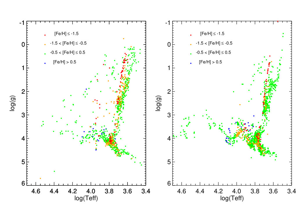 Figure 2
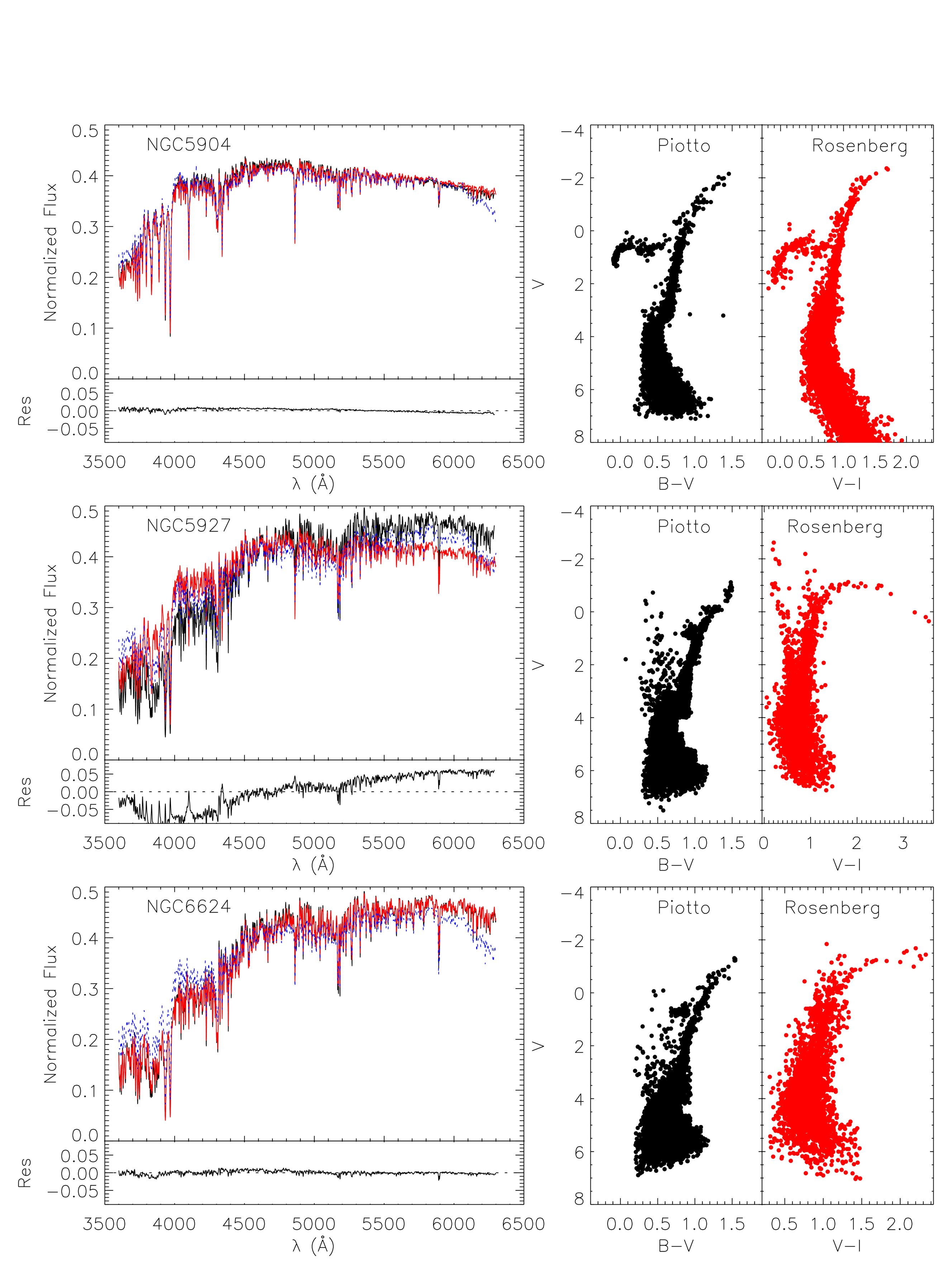 Figure 3
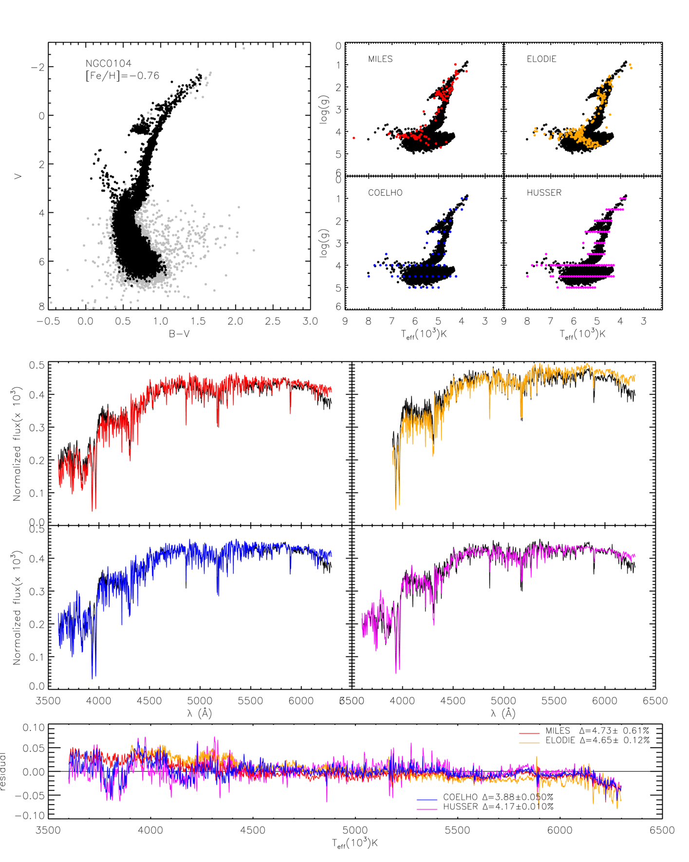 Figure 4
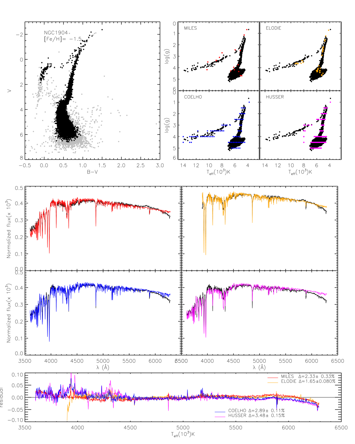 Figure 5
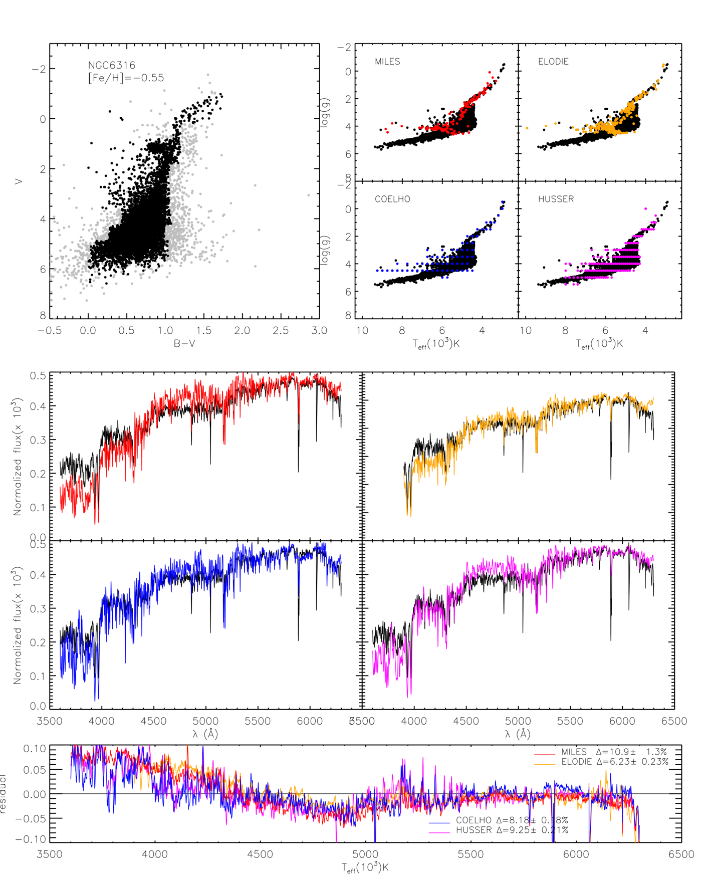 Figure 6
| ID | No.stars brigher | No. stars removed | No. stars removed | (%) | (%) | (%) |
|---|---|---|---|---|---|---|
| than Top MS | by Mag error | by wrong phase | no removal | removal mag | Final | |
| NGC0104 | 2468 | 68( 2.76%) | 8( 0.32%) | 4.61 | 4.11 | 3.88 |
| NGC1851 | 3117 | 328(10.52%) | 70( 2.25%) | 3.90 | 2.58 | 2.67 |
| NGC1904 | 1596 | 30( 1.88%) | 124( 7.77%) | 2.71 | 2.23 | 2.89 |
| NGC2808 | 6892 | 546( 7.92%) | 189( 2.74%) | 3.05 | 2.49 | 2.70 |
| NGC3201 | 349 | 1( 0.29%) | 0( 0.00%) | 3.74 | 3.70 | 3.70 |
| NGC5904 | 1698 | 103( 6.07%) | 71( 4.18%) | 1.92 | 2.43 | 2.00 |
| NGC5927 | 2433 | 29( 1.19%) | 82( 3.37%) | 32.67 | 8.50 | 7.21 |
| NGC5946 | 1338 | 32( 2.39%) | 80( 5.98%) | 43.24 | 6.23 | 6.35 |
| NGC5986 | 2086 | 65( 3.12%) | 137( 6.57%) | 6.15 | 4.85 | 4.49 |
| NGC6171 | 521 | 35( 6.72%) | 12( 2.30%) | 5.87 | 5.82 | 5.81 |
| NGC6218 | 477 | 10( 2.10%) | 14( 2.94%) | 6.79 | 2.65 | 2.86 |
| NGC6235 | 498 | 3( 0.60%) | 24( 4.82%) | 4.30 | 3.51 | 3.48 |
| NGC6266 | 3887 | 117( 3.01%) | 127( 3.27%) | 4.35 | 4.24 | 4.06 |
| NGC6284 | 1631 | 42( 2.58%) | 56( 3.43%) | 5.50 | 4.71 | 4.36 |
| NGC6304 | 1515 | 11( 0.73%) | 149( 9.83%) | 8.62 | 8.52 | 7.92 |
| NGC6316 | 1865 | 23( 1.23%) | 264(14.16%) | 8.40 | 8.78 | 8.18 |
| NGC6342 | 470 | 2( 0.43%) | 15( 3.19%) | 14.68 | 14.86 | 14.26 |
| NGC6356 | 3468 | 53( 1.53%) | 69( 1.99%) | 6.37 | 6.69 | 6.45 |
| NGC6362 | 483 | 7( 1.45%) | 11( 2.28%) | 6.06 | 3.73 | 3.47 |
| NGC6388 | 7999 | 253( 3.16%) | 74( 0.93%) | 6.47 | 6.78 | 6.48 |
| NGC6441 | 7902 | 150( 1.90%) | 99( 1.25%) | 7.55 | 7.86 | 7.92 |
| NGC6522 | 2257 | 13( 0.58%) | 373(16.53%) | 4.20 | 4.13 | 4.30 |
| NGC6544 | 505 | 11( 2.18%) | 124(24.55%) | 12.33 | 12.43 | 9.92 |
| NGC6569 | 2128 | 37( 1.74%) | 179( 8.41%) | 8.47 | 8.84 | 8.64 |
| NGC6624 | 2581 | 56( 2.17%) | 43( 1.67%) | 8.36 | 8.57 | 8.71 |
| NGC6637 | 1932 | 304(15.73%) | 20( 1.04%) | 4.60 | 4.58 | 4.63 |
| NGC6638 | 1397 | 58( 4.15%) | 117( 8.38%) | 4.50 | 4.49 | 4.54 |
| NGC6652 | 925 | 4( 0.43%) | 223(24.11%) | 3.33 | 3.34 | 3.78 |
| NGC6723 | 1126 | 21( 1.87%) | 74( 6.57%) | 2.92 | 2.92 | 2.98 |
| NGC7089 | 2868 | 38( 1.32%) | 49( 1.71%) | 2.03 | 2.09 | 2.19 |
| (Full range) | (Short range) | ||||||
|---|---|---|---|---|---|---|---|
| ID | MILES | COELHO | HUSSER | ELODIE | MILES | COELHO | HUSSER |
| NGC0104 | 4.21 0.14 | 3.880.050 | 4.260.030 | 4.65 0.12 | 2.830.090 | 3.090.050 | 3.760.040 |
| NGC1851 | 3.34 0.15 | 2.67 0.18 | 4.59 0.22 | 2.25 0.18 | 2.120.070 | 2.41 0.22 | 3.82 0.23 |
| NGC1904 | 2.300.090 | 2.89 0.11 | 3.24 0.16 | 1.650.080 | 1.760.030 | 2.41 0.10 | 2.88 0.13 |
| NGC2808 | 3.39 0.10 | 2.700.050 | 4.44 0.10 | 2.340.070 | 2.130.050 | 2.000.050 | 3.110.070 |
| NGC3201 | 3.49 0.28 | 3.700.080 | 3.700.030 | 4.42 0.21 | 3.53 0.28 | 3.30 0.15 | 3.330.060 |
| NGC5904 | 2.55 0.19 | 2.00 0.23 | 2.410.080 | 1.76 0.19 | 1.79 0.22 | 1.73 0.27 | 2.22 0.10 |
| NGC5927 | 9.88 0.38 | 7.21 0.25 | 8.37 0.31 | 7.67 0.25 | 6.28 0.32 | 4.98 0.18 | 5.67 0.19 |
| NGC5946 | 6.05 0.16 | 6.35 0.38 | 6.47 0.20 | 5.83 0.38 | 4.99 0.19 | 5.21 0.40 | 5.34 0.17 |
| NGC5986 | 3.92 0.17 | 4.49 0.29 | 5.07 0.29 | 2.57 0.17 | 2.66 0.10 | 3.34 0.29 | 4.00 0.30 |
| NGC6171 | 6.59 0.12 | 5.810.060 | 6.56 0.16 | 4.26 0.10 | 5.07 0.13 | 4.540.060 | 4.920.060 |
| NGC6218 | 2.90 0.17 | 2.86 0.21 | 3.73 0.28 | 1.980.030 | 2.090.040 | 2.34 0.13 | 3.22 0.16 |
| NGC6235 | 3.84 0.29 | 3.48 0.58 | 4.15 0.48 | 2.85 0.45 | 3.12 0.17 | 3.00 0.53 | 3.55 0.35 |
| NGC6266 | 4.96 0.16 | 4.06 0.17 | 4.96 0.17 | 2.830.070 | 3.300.050 | 3.01 0.17 | 3.73 0.14 |
| NGC6284 | 4.65 0.31 | 4.36 0.20 | 5.92 0.25 | 2.60 0.32 | 3.40 0.17 | 3.69 0.21 | 4.98 0.21 |
| NGC6304 | 8.24 0.34 | 7.92 0.29 | 9.11 0.30 | 7.20 0.23 | 5.41 0.24 | 5.67 0.22 | 6.42 0.23 |
| NGC6316 | 9.70 0.29 | 8.18 0.18 | 9.73 0.25 | 6.23 0.23 | 6.25 0.16 | 5.73 0.21 | 6.27 0.25 |
| NGC6342 | 14.3 0.45 | 14.2 0.43 | 15.3 0.38 | 11.8 0.29 | 10.2 0.35 | 10.6 0.32 | 11.2 0.32 |
| NGC6356 | 7.83 0.22 | 6.45 0.18 | 7.79 0.23 | 6.56 0.14 | 4.81 0.15 | 4.50 0.14 | 5.26 0.13 |
| NGC6362 | 5.29 0.39 | 3.47 0.19 | 4.23 0.38 | 4.73 0.48 | 3.21 0.18 | 2.65 0.18 | 3.23 0.29 |
| NGC6388 | 7.60 0.25 | 6.48 0.13 | 8.18 0.16 | 7.45 0.14 | 4.94 0.19 | 5.14 0.14 | 5.63 0.13 |
| NGC6441 | 10.5 0.30 | 7.92 0.20 | 9.83 0.23 | 8.51 0.14 | 6.82 0.20 | 6.13 0.17 | 6.52 0.15 |
| NGC6522 | 4.46 0.28 | 4.30 0.35 | 4.33 0.15 | 5.52 0.38 | 4.55 0.26 | 3.98 0.36 | 3.90 0.20 |
| NGC6544 | 9.96 0.21 | 9.92 0.17 | 8.97 0.13 | 11.6 0.17 | 10.2 0.24 | 9.67 0.29 | 8.73 0.21 |
| NGC6569 | 10.0 0.22 | 8.64 0.39 | 9.53 0.29 | 8.52 0.20 | 5.82 0.16 | 5.63 0.18 | 6.41 0.24 |
| NGC6624 | 11.0 0.35 | 8.71 0.37 | 9.92 0.46 | 9.68 0.26 | 7.52 0.34 | 6.47 0.29 | 7.15 0.35 |
| NGC6637 | 5.54 0.12 | 4.63 0.31 | 6.79 0.19 | 3.78 0.19 | 3.590.090 | 3.86 0.31 | 4.44 0.10 |
| NGC6638 | 5.30 0.12 | 4.54 0.36 | 4.710.090 | 3.540.090 | 3.59 0.12 | 3.75 0.37 | 3.66 0.11 |
| NGC6652 | 3.18 0.22 | 3.78 0.28 | 4.92 0.34 | 4.13 0.15 | 2.50 0.17 | 3.46 0.34 | 4.76 0.46 |
| NGC6723 | 3.66 0.15 | 2.980.080 | 3.78 0.18 | 2.24 0.14 | 2.440.070 | 2.430.040 | 3.00 0.10 |
| NGC7089 | 2.04 0.11 | 2.19 0.11 | 2.89 0.16 | 1.61 0.21 | 1.740.050 | 1.99 0.11 | 2.64 0.14 |
Peer Reviews
No public reviews on file for this paper yet. If you reviewed it on a platform where reviews are public (OpenReview, ICLR, NeurIPS, ICML), you can paste yours below so the community can read it here.
Videos
No videos yet. Explain this paper in a talk, walkthrough, or lecture? Add one.
Testing Stellar Population Fitting Ingredients with Globular Clusters I: Stellar Libraries.
Lucimara P. Martins,1 Círia Lima-Dias,1,3 Paula R. T. Coelho2 and Tatiana F. Laganá 1
1NAT–Universidade Cruzeiro do Sul, Rua Galvão Bueno, 868, 01506-000, Sao Paulo, SP, Brazil
2IAG–Universidade de São Paulo, Rua do Matão, 1226, 05508-090, Sao Paulo, SP, Brazil
3Departamento de Física, Universidad de La Serena, Av. Cisternas 1200, La Serena, Chile E-mail: [email protected]
(Accepted XXX. Received YYY; in original form ZZZ)
Abstract
The integrated spectra of stellar systems contain a wealth of information, and its analysis can reveal fundamental parameters such as metallicity, age and star formation history. Widely used methods to analyze these spectra are based on comparing the galaxy spectra to stellar population (SP) models. Despite being a powerful tool, SP models contain many ingredients, each with their assumptions and uncertainties. Among the several possible sources of uncertainties, it is not straightforward to identify which ingredient dominates the errors in the models. In this work we propose a study of one of the SP model ingredients – the spectral stellar libraries – independently of the other ingredients. To that aim, we will use the integrated spectra of globular clusters which have color-magnitude diagrams (CMDs) available. From these CMDs it is possible to model the integrated spectra of these objects without having to adopt – or make assumptions – on the other two main ingredients of SP models, evolutionary tracks or an IMF. Here we tested four widely used stellar libraries. We found that the libraries are able to reproduce the integrated spectra of 18 of the 30 cluster spectra inside a mean flux uncertainty of 5%. For the larger wavelength range tested, a theoretical library outperforms the empirical ones in the comparison. Without the blue part of the spectra, empirical libraries fare better than the theoretical, in particular when individual features are concerned. However, the results are promising for theoretical libraries, which are equally efficient to reproduce the whole spectrum.
keywords:
Stars: general – Stars: fundamental parameters – Astronomical database: miscellaneous – Globular clusters: general –
††pubyear: 2018††pagerange: Testing Stellar Population Fitting Ingredients with Globular Clusters I: Stellar Libraries.–A
1 Introduction
Most of the light in the universe comes from stars. Our understanding of stars and stellar evolution evolved significantly over the last decades, from the UV to the near-IR, mostly by observing, interpreting and modeling the stars of our solar vicinity. However, with the exception of the closest galaxies, we still cannot resolve stars individually down to the turn-off (TO) and below (for galaxies beyond the local group we can resolve stars in the bright Red Giant Branch (RGB), down to the red clump - Rejkuba et al. (e.g. 2011)), at least until the advent of the Extremely Large Telescopes (Olsen et al., 2003). As such, when we observe a galaxy, its spectrum will contain the contribution of all emitting objects in this galaxy, including all its stars. One of the major challenges that astronomers face today is to extract physical, chemical and evolutionary information about the galaxy from this integrated spectrum.
Several techniques are available to extract information from integrated spectra, mostly involving the comparison of the observations to stellar population model libraries with a wide range of ages and metallicities (e.g. Panter et al., 2003; Cid Fernandes et al., 2005; Mathis et al., 2006; Ocvirk et al., 2006a, b; Walcher et al., 2006; Koleva et al., 2008; Coelho et al., 2009; Cezario et al., 2013; Kuntschner et al., 2001; Ocvirk et al., 2006c; Wolf et al., 2007; Koleva et al., 2008). The simplest models in this context are the simple stellar population (SSP) models, which are spectra built theoretically using as ingredients isochrones, an initial mass function (IMF), and a library of stellar spectra (e.g. Bruzual A., 1983; Arimoto & Yoshii, 1986; Guiderdoni & Rocca-Volmerange, 1987; Bressan et al., 1994; Cerviño & Mas-Hesse, 1994; Worthey, 1994; Vazdekis et al., 1996; Fioc & Rocca-Volmerange, 1997; Kodama & Arimoto, 1997; Maraston, 1998; Leitherer et al., 1999; Buzzoni, 2002; Bruzual & Charlot, 2003; Jimenez et al., 2004; Le Borgne et al., 2004; Delgado et al., 2005; Maraston, 2005; Schiavon et al., 2006; Coelho et al., 2007; Conroy & Gunn, 2010; Vazdekis et al., 2010; Blakeslee et al., 2010; Meneses-Goytia et al., 2015).
Stellar isochrones depend on an extensive grid of evolutionary stellar tracks, which model the stellar evolution with a given initial mass and chemical composition. In the last decades there were major efforts from different groups to supply homogeneous sets of evolutionary tracks like Padova (Marigo & Girardi, 2007; Marigo et al., 2008), Geneva (Lejeune & Schaerer, 2001), Yale (Demarque et al., 2004), MPA (Weiss & Schlattl, 2008) and BaSTI (Pietrinferni et al., 2009). Evolutionary effects of chemical variations like -enhancement (e.g. Salasnich et al., 2000; Pietrinferni et al., 2009) or individual element variations (e.g. Dotter et al., 2007) were also investigated. Still, problems exist in this field, with different treatments by different groups leading to different evolutionary tracks, even when using the same input parameters (Walcher et al., 2011; Martins et al., 2013).
The IMF gives the number of stars of each given mass for a given star formation episode. There are many different recipes for the IMF used in the literature, being the most common ones the Salpeter (1955), Kroupa & Boily (2002) and Chabrier (2003). Our knowledge of the IMF is based on our interpretation of observations and many assumptions, such as that the IMF is universal and constant in time. Doubts about these assumptions are still in debate today and there is a lot of room for improvement (Chiappini et al., 2000; Chieffi & Limongi, 2002; Bastian et al., 2010; Calura et al., 2010; Bonatto & Bica, 2012).
Stellar libraries can be either empirical or theoretical. Empirical libraries are based on observational data, which implies that all features contained in the resulting SSP spectra will be real. The disadvantage, however, is that these libraries are biased towards the star formation and chemical enrichment histories of the solar neighborhood, the Small and Large Magellanic Clouds or Galactic Globular Clusters (GCs), limiting the coverage and sampling of the HR diagram. Theoretical libraries do not have this setback, since it is possible to generate stellar spectra with virtually any temperature or metallicity desired, in any wavelength range, covering the whole parameter space. Of course, this also comes with a limitation, since they are build from models which are always based on physics approximations and simplifications (Bessell et al., 1998; Kučinskas et al., 2005; Kurucz, 2006; Martins & Coelho, 2007; Bertone et al., 2008; Coelho et al., 2009; Plez, 2011; Lebzelter et al., 2012; Sansom et al., 2013; Kitamura et al., 2017).
Given all the ingredients required to build a SSP spectrum and the approximations in each of them, it is very difficult to identify where the major problems are when models cannot reproduce the observed spectra of galaxies (e.g. Chen & Han, 2010). Ideally, each ingredient should be tested separately in order to better understand where models fail and where they work, and to be able to choose among the many options available.
With this in mind, this is the first paper of a series which use GCs integrated spectra to test individually the ingredients used in the SSP construction. In this first paper we test some of the currently available spectral stellar libraries.
GCs are ideal objects to study stellar populations. They are objects where we can resolve individual stars and as such obtain their color-magnitude diagrams (CMD). From resolved-stars studies it is possible to obtain ages and metallicities through methods more accurate than the ones using integrated light. From the CMD it is also possible to model the integrated spectra of the cluster using only a library of stellar spectra, without the need to adopt isochrones or IMF. In this work we use a sample of GCs from Schiavon et al. (2004), for which both CMDs and integrated spectra are available, to test how well empirical and theoretical libraries are able to reproduce the integrated spectra of Galactic GCs. This work is organized as follows: in §2 we give an overview of what will be done in this work, in §3 we describe the GC sample; in §4 we present the CMDs and how we derive the stellar parameters for each star in the GC; in §5 we describe the stellar libraries to be tested; in §6 we explain the construction of the synthetic integrated spectra for each GC; in §7 we present our results, and in §8 our conclusions.
2 Methodology
The objective of this work is to test how efficiently libraries of stellar spectra can be used to produce a synthetic integrated spectra able to reproduce the spectra of GCs, without any assumption of an IMF or isochrone. To that aim, we built a synthetic spectrum for each GC, based on CMD data and a stellar spectral library, and compare our synthetic spectrum to an observed one from literature.
To build the synthetic integrated spectrum of a GC, each star in a given CMD will be associated to a Teff and a log g using color relations (the metallicity assumed to be that of the cluster, as reported in literature). In turn, each combination of Teff, log g and [Fe/H] will then be associated to a stellar spectrum in the stellar library. Our synthetic integrated spectrum will then be created by summing up the selected stellar spectra from the stellar library, weighted by their absolute magnitude as given in the CMD. This synthetic integrated spectrum can then be compared to the observed integrated observed spectrum of the GC. The quality of the synthetic spectrum was quantified by a total difference in flux with the observed spectrum defined in Sect. 6 of this paper, called . In the next sections we will detail each step of the work described here.
3 The Sample
This work is based on 30 Galactic GCs which have publicly available integrated spectra and CMDs from the literature: integrated spectra from Schiavon et al. (2005) and CMDs from Piotto et al. (2002). Table 1 shows some of the GCs main properties, obtained from Piotto et al. (2002), except for col. 5, the heliocentric distance, which was obtained from Harris (1996). Their integrated spectra were obtained from Schiavon et al. (2005)111Available for download at https://www.noao.edu/ggclib/., who observed 40 GCs from our galaxy with the 4m Blanco Telescope at Cerro Tololo, in the Inter-American Observatory (CTIO). The spectra range from 3350 to 6430 Å, with a resolution of 3.1Å (FWHM), and a S/N from 50 to 240 at 4000 Å and 125 to 500 in 5000 Å. Due to the extended nature of the clusters, the integrated spectra were obtained by drifting the spectrograph slit across their core diameter. This ensured that the integrated spectra contained the contribution from stars all over the cluster, avoiding selection effects that could arise by observing only a region of the GC. We corrected the spectra for reddening using the Cardelli et al. (1989) extinction law, where the E(B-V) was adopted from Table 1 and RV= 3.1.
Schiavon et al. (2005) gives the references for the CMDs of all 40 GCs. In search of homogeneity, we choose the reference with the larger number of CMDs observed. This led us to Piotto et al. (2002), which has B and V data for 30 of the 40 GCs from Schiavon et al. (2005). They observed 74 Galactic GCs with HST/WFPC2 camera in the F439W and F555W bands, and transformed them to the standard Johnson B and V systems. They produced CMDs down to a little below the main-sequence turnoff for all their clusters, all measured and reduced in a uniform way.
3.1 Caveats
The study presented in this paper is based on the assumption that the CMD from Piotto et al. (2002) and the integrated spectra from Schiavon et al. (2005) observed similar populations in each cluster.
We tested this hypothesis by building the luminosity function of the GCs from the CMDs directly, and the luminosity function implicit in the integrated spectra by Schiavon et al. (2005) using their reported values regarding the field which was observed for each GC. To accomplish this, we used the CCD coordinates and the pixel scale of the CMDs observations given by Piotto et al. (2002). The distributions are almost always similar (the exceptions being clusters with few stars). This test gives us confidence that for most clusters, photometric and spectroscopic data are sampling very similar populations. It is important, however, to note here that although Schiavon et al. (2005) took great care to ensure the representativity of the integrated spectrum of each cluster, they are still subject to stochastic effects. Under some circumstances, the influence of a single star can greatly affect the integrated light of the cluster, even when the entire core diameter is covered. In fact, any bright star in the cluster with a very different spectrum from the rest of the cluster can affect the integrated spectrum. The authors tried to account for this with a variance-weighted extraction, where any bright star in the cluster with a very different spectrum from the rest of the cluster was a target for removal, but for the less concentrated clusters this might be an issue.
Also we should consider that GCs are systems undergoing dynamical evolution. In the Milky Way there are numerous GCs that currently experience or recently passed through a phase of core collapse. This means that the less massive stars migrate to the outer parts of the cluster, leaving the brighter stars more concentrated in the core region. If the segregation is too great and most of the less massive stars or of a particular important phase are absent in the core, the integrated spectrum would not be compatible with the synthetic spectrum from the CMD. However, only 7 of the 30 GCs of this sample are characterized as core collapsed according to Piotto et al. (2002). These are marked as "cc" in column 4 of Table 1.
4 CMDs and Stellar Atmospheric Parameters
The B and V apparent magnitudes supplied by Piotto et al. (2002) were converted to absolute magnitudes using the heliocentric distances given by Harris (1996) (column 5 of Table 1) and the extinction values from Piotto et al. (2002) (column 6 of Table 1).
We performed a manual cleaning of the CMDs by adopting the following strategy: first, all stars with magnitude errors larger than 0.15 were removed. We then checked for outliers in the remaining stars. The main sequence, for example, is a well defined region in the CMD. Stars in the bottom of the CMD that are outside this region and clearly not in any other evolutionary stage can be considered contamination. To eliminate these stars the MS was divided in 7 equal intervals in V. For each of these intervals we obtained the average B-V value, which defined the MS locus. We allowed for stars in a 4 interval to be kept for each of these intervals, and the stars outside this range were removed. Outside the MS the procedure was a little more subjective. We visually inspected each of the CMDs and manually removed stars that were clear outliers, which means that they were clearly not in any of the known locus for stellar phases in the CMD.
We report in Table 2 how many stars were removed by each of these processes. Column 2 of this table shows the number of stars brighter than the top of the MS, which are the stars that most contribute to the integrated spectrum. Column 3 shows how many stars were removed by the magnitude errors and the cleaning of the MS. Column 4 shows how many stars were removed because they were outliers. The effect of these removals can be seen in the last three columns of this table. These columns show the value (which represents the total difference in flux between observed and synthetic spectra) for the Coelho library (as an example), using the CMD without any cleaning, cleaning only the MS and the magnitude errors, and for the final cleaned CMD. The definition of and its significance are explained later in Sect. 6 and 7, but the objective here is to show that, although changes in the synthetic spectra are obtained by this cleaning process, the overall results do not change. Figure 1 shows, as an example, the CMD of NGC 1851 before the cleaning process (left panel), and after the cleaning process (right panel).
The fact that we are still able to reproduce the observed spectra (see Sect. 7) indicates that many of these stars will indeed not be present in the integrated spectra, which was obtained only for the core region of the GCs, and the ones that could not be avoided are just few enough that the integrated spectra would not be affected by them. The cases where this might not be true are the GCs located in the direction of the Galactic Bulge, where contamination might be strong. There are 11 GCs with this problem, and their CMDs are indeed clearly strongly contaminated. We tried to remove outliers stars as best as possible.
Another important aspect of the CMD that has to be taken into account is that there will be low mass stars below the limits of the observations that are not taken into account in this work. However, all CMDs have stars well bellow the TO, and the differences in magnitude between the faintest star and the brightest are, on average, around 8 magnitudes. This means that these stars will contribute very little to the integrated flux. To test that we removed the bottom stars up to 1 magnitude from the fainter star of each CMD and found that their contribution is around 0.02% of the integrated flux. This means these low mass stars will not important for the integrated flux, at least in this wavelength range.
Stars in the spectral stellar library are characterized by their effective temperature (Teff), surface gravity () and metallicity ([Fe/H]) values. We assumed that all the stars in a given cluster have the same metallicity, so this parameter was defined by the [Fe/H] of the cluster given in Table 1. The next step is then to convert the CMD into a Teff x plane.
4.1 Atmospheric parameters of the stars in the CMD
We used the color-temperature relation from Worthey & Lee (2011) to estimate Teff for each star in the CMD from its (B–V) color. Using basic definitions of gravitational force and luminosity, it is easy to deduce that can be obtained from:
[TABLE]
where ⊙ is the solar surface gravity, M*⋆* and M*⊙* are the masses of the star and the Sun, respectively, and L*⋆* and L*⊙* the luminosities of the star and the Sun, respectively.
The luminosity of each star can be obtained from the absolute V magnitude and a bolometric correction (BC):
[TABLE]
where Mbol⊙ is the bolometric magnitude of the Sun. The BC values were also obtained from the relations presented in Worthey & Lee (2011).
The stellar masses necessary for equation 1 can be obtained from a luminosity-mass relation. We used three different relations for different regions of the CMD:
- •
for the stars in the MS we adopted L M4 ;
- •
for the giant branch stars we assumed that the mass was equal to the average mass of the top of the MS, and;
- •
for the horizontal branch stars we considered an average value of 0.8 M*⊙*, following Salgado et al. (2013).
.
We compared these assumptions with the model predictions from BaSTi isochrones (Pietrinferni et al., 2009). We find that the L M4 is a reasonable approximation of the main sequence, although it overestimates the mass near the TO by a maximum of about 1 M*⊙*, which translates into an uncertainty of 0.3 dex in log g. The models show that indeed the masses for post-MS phases are similar to the mass of the TO. Masses of the HB stars cannot be interpreted easily, as we cannot yet model accurately the mass loss in the RGB and thus the HB morphology. Models show that masses tend to be constant along the HB, so we believe our approach here is reasonable.
5 Stellar Libraries
We choose in this work to test four stellar libraries, two empirical and two theoretical, which we found representative of the several available in literature. They were chosen primarily by their potential application for stellar population synthesis (broad stellar parameter coverage), and modern input physics.
5.1 MILES
The MILES library (Sánchez-Blázquez et al., 2006) is an empirical stellar library built primarily for stellar population modeling. The spectra were obtained at Roque de los Muchachos observatory, covering from 3525 to 7500 Å, with a resolution of 2.5 0.7 Å(FWHM, Falcón-Barroso et al., 2011). It has 985 stars with a large selection of luminosities and spectral types, with a coverage of -2.7 to 1.0 dex in [Fe/H], 2819 to 36000K in Teff and 0 to 5.5 dex in . The atmospheric parameters of the stars were derived by Cenarro et al. (2007) and revised by Prugniel et al. (2011) and Sharma et al. (2016).
We did not use all 985 stars from the available library. We removed stars with emission lines, with E(B-V)0.1, stars without [Fe/H] estimations and binaries. This list of stars was shared with us by Christopher Barber through private communication (Barber et al., 2014). We also removed some with clearly problematic spectra (private communication from Coelho, P. & Bruzual, C.). Our final MILES sample contains 935 stars. The distribution of the MILES stars in the Teff vs. plane is shown in Figure 2.
5.2 ELODIE
The ELODIE library (Soubiran et al., 1998; Prugniel & Soubiran, 2001; Le Borgne et al., 2004) is a stellar database containing 1959 spectra from 1503 different stars, which were observed with the echelle spectrograph ELODIE using the 1.93m telescope at the Observatoire de Haute Provence. It has been updated since the first publication, improving considerably the parameter space coverage. The data reduction was also revised, in particular, the flux calibration. The spectra are available in two different spectral resolutions: high-resolution (R = 42000) and low-resolution (R = 10000 at = 550nm, or FWHM 0.55 Å). The wavelength coverage is = 3900 - 6800 Å. The HR diagram coverage is extensive for an empirical library: 0.27 to 4.97 dex in , 3185K to 55200K in Teff and -3.21 to 1.62 dex in [Fe/H]. Each of the atmospheric parameters for the stars have a quality flag, and we choose to eliminate from our work stars with poor determinations in Teff and . The total number of spectra left was 1783. The distribution of the Elodie stars in the Teff vs. log g plane is shown in Figure 2.
5.3 COELHO
Theoretical libraries are of fundamental importance to cover parameter regions that empirical libraries are not able to. Coelho (2014) provides a theoretical library covering from 2500 to 9000 Å. It has a coverage of 3000 to 25000K in Teff and -0.5 to 5.5 dex in , regularly spaced. The spectra for stars with Teff 4000 K were calculated using ATLAS9 model atmospheres (Kurucz, 1970; Sbordone et al., 2004) and stars with Teff 4000 K, MARCS model atmospheres were used (Gustafsson et al., 2008). The spectra were computed using a large and carefully updated atomic and molecular opacity database. The spectral synthesis code used was SYNTHE (Kurucz & Avrett, 1981).
Coelho (2014) library has 12 different chemical mixtures. For this work we only used 4, which are the sub-solar metallicities (because all GCs used in this work have [Fe/H]0) with [/Fe] = 0.4, since we know GCs are usually enhanced.
5.4 HUSSER
Husser et al. (2013) provides a theoretical library built using version 16 of the stellar atmosphere code PHOENIX (Hauschildt et al., 1999). The atmosphere models for this library were created with a new equation of state and up-to-date atomic and molecular line lists. They also used spherical geometry from the main sequence to giants, guaranteeing a consistent grid. The spectra cover the wavelength range 500 Å to 5.5 m. It has a coverage of 2300 to 12000K in Teff, 0.0 to 6.0 dex in , -4.0 to +1.0 dex in [Fe/H] and -0.2 to 1.2 dex in [/Fe]. However, for [/Fe] 0.4 the coverage in Teff and in [Fe/H] is smaller. Because of this limitation we used only the solar [/Fe] value in this work.
6 Construction of the Synthetic Integrated Spectra
Building a synthetic spectrum for each GC and with stellar library begins with selecting, in the spectral library, the stars with the same metallicity of the cluster. For the empirical libraries, this was done by selecting stars within 0.5 dex of the GC metallicity. This value was chosen as the best compromise to keep a representative number of stars for each GC. For the theoretical libraries, we choose stars with the [Fe/H] values closest to that of the GC.
After that, we searched the stellar libraries for a correspondence for each observed star in a given GC. That was done by calculating a “distance" (d) of each cluster star in the log(g) x Teff plane from all stars in a given library with the correct metallicity, and choosing for each one the library star with the smallest d. This is calculated by (Martins & Coelho, 2007):
[TABLE]
where TB and TGC are the effective temperatures of the stellar library and the GC stars, respectively, and B and GC are the surface gravities of the stellar library and the GC stars, respectively. Because the number of stars in the libraries are limited, there will be stars in the libraries which represent more than one star in each GC. Also, when the libraries do not cover the extremes of the parameter space, like very cool bright stars and very hot stars, the star with the smallest is chosen to represent it. We performed neither interpolation nor extrapolation in this work.
In the final step, a synthetic GC spectrum is built through the linear combination of the individual stellar spectra:
[TABLE]
where is the synthetic integrated spectrum of the GC, F*⋆i* is the stellar library spectrum that will represent the ith star of the GC and is the total number of stars of the GC. The stellar spectra of each library were convolved to the spectral resolution of the observed integrated spectra of the GC before starting this process. Ci is the weight given to each stellar spectrum, given by:
[TABLE]
where Fλi is the stellar spectrum normalized to , multiplied by the transmission curve of the Johnson V filter, and Vi is the absolute magnitude of the ith star. This means that brighter stars will contribute more to the integrated spectrum than dimmer ones, as expected.
To evaluate the quality of each synthetic integrated spectrum in reproducing the observed spectra as observed by Schiavon et al. (2005), we computed the absolute average deviation for each combination of GC and stellar library, defined by:
[TABLE]
where N is the number of pixels in the spectra, Oi is the observed flux at the pixel i and Mi is the synthetic flux obtained at pixel i. All spectra, both synthetic and observed, were re-sampled to 1Å, to have the same number of pixels. All integrated spectra, both synthetic and observed, were normalized to before comparison.
6.1 Uncertainties
This technique of computing the synthetic integrated spectra involves, as any other, many assumptions. We believe that the main one in this case is the conversion of the stellar magnitudes and colors of the CMD into Teff and . Two main effects might be playing a role here: (1) the choice of the filters used to construct the CMD, and (2) the errors in the magnitude measurements. We tried to access how each of these problems would affect the final synthetic integrated spectra.
To evaluate (1) we obtained CMDs from Rosenberg et al. (2000a, b) for clusters in common with our sample. These authors obtained V and I for 52 Galactic GCs, 14 in common with the ones presented here. Their data was obtained using the DUTCH 91cm telescope in La Silla, Chile, and the 1m Jacobus Kapteyn telescope, in Roque de los Muchachos, Spain.
We used the same procedure already described above to produce synthetic integrated spectra using the Rosenberg et al. data, and compared with the ones produced with the Piotto et al. data for the clusters in common. In general, the CMDs using the (V-I) color have a larger number of fainter stars, but they have little influence in the final spectrum.
The CMDs using the (B-V) color have more stars in general, and in particular, tend to have more extended horizontal branches and more blue stragglers. Figure 3 shows three representative examples. When CMDs with (V-I) and (B-V) are similar, the synthetic integrated spectra generated with them are also similar. This is the case of NGC 1904, NGC 5904 (shown as example in the top panel of Figure 3) and NGC 6362.
For some of the clusters, although the CMDs are not well defined, and do not look so similar, the final synthetic integrated spectra from each color remain similar. NGC 6624, in the bottom panel of Figure 3 is an example of such case. This also happens for NGC 104, NGC 3201 and NGC 6637.
For the other seven clusters, the CMDs in (B-V) differ significantly from the one in (V-I). This happens because the CMDs are confusing and/or too contaminated, as is the case of NGC 5927, shown in the middle panel of Figure 3, or because the (B-V) CMD has many more blue stragglers or a much broader AGB. The differences between the filters might also be related to the contamination of the GCs by background/foreground stars. This will be more problematic for clusters in the Galactic Bulge direction, where the contamination would be strongest. However, from these 14 GCs compared here, only one (NGC 5927) is in this direction. Therefore we believe contamination is not an issue for this comparison. From the seven clusters where the synthetic integrated spectrum generated by each color differ, four (NGC 1851, NGC 5927, NGC 6171 and NGC 6638) better represent the observed with spectra when using the (B-V) CMD and three (NGC 5986, NGC 6218 and NGC 6723) when using the (V-I) CMD. There seems to be no clear pattern for these differences, and it could only be explained in terms of stochastic effects in the star sample, both for the observed spectrum and for the CMDs.
To evaluate (2) we used the uncertainties in the magnitudes to generate new CMDs, varying the magnitudes of each star randomly inside the uncertainty interval. We generated 100 new CMDs for each GC, and for each of them a new synthetic integrated spectrum and . With that we have an standard deviation for , which gives us an idea of how much the errors in the magnitudes affect the whole process. These errors vary from 2% to 17% and are presented together with the results for in Table 3.
7 Results and Analysis
Our quantitative results are presented in Table 3. In Figures 4 to 6 we show some representative examples of the synthetic integrated spectra in comparison with the observed spectra. Similar figures for all GCs can be found in the online material.
The libraries MILES, Coelho and Husser cover almost the whole wavelength range of the observations (MILES library starts at 3525 Å, which sets the lower limit in Å in our comparisons). The Elodie library, however, starts at 3900 Å. Although the value takes into account the smaller number of points for the spectra constructed with this library, the from ELODIE are not directly comparable to the of the other libraries. This happens because the blue part of all observed spectra is most difficult to reproduce, raising the values for the libraries that cover this region. Because of that, we also calculated alternative values for MILES, Coelho and Husser but with the same wavelength range as Elodie, which can then be directly compared.
We divided the quality of the synthetic integrated spectra into three categories, based on the smallest value obtained for the full wavelength range: very good, good and bad fits. Very good fits are the ones with 3% (7 clusters), good fits have 3% 5% (11 clusters) and bad fits are the ones with 5% (12 clusters). We are thus able to reproduce 18 of the 30 (60%) cluster integrated spectra inside a mean flux uncertainty of 5%. However, a deeper analysis reveals many interesting details about these results.
First, all the clusters in the very good fit category have well defined and well behaved CMDs. Figure 4 shows the results for NGC 1904 as an example of this category. Clusters in the good category start to have different kinds of CMDs, either by having broader main sequences, broad RGB, holes in regions like the AGB, RGB or HB, and even very unconventional CMDs (very broad or indistinguishable MS, double red giant branches or MS, etc.) maybe due to a composite population, which is the case of NGC 6522, for example. Figure 5 shows the results for NGC 104 as an example of this category. For the clusters in the bad fit category, CMDs are all problematic. Some have clearly composite populations (e.g. NGC 5946), others look strongly contaminated (e.g. NGC 6316) and a few have very few stars in comparison with the others (e.g. NGC 6171), which makes them more susceptible to stochastic effects, both in the CMD and in the integrated spectra. One of them, NGC 6544 seems to be a particular case, where the integrated observed spectrum looks very strange and incompatible with the CMD, even considering some stochastic effects. As mentioned in Sect. 3.1, some of the clusters of our sample are core collapsed GCs. We looked for a correlation between this characteristic and the quality of the synthetic spectra, and found none. Only 4 of the 12 GCs with bad fits are core collapsed. The other 3 core collapsed GCs are the in good fits category. NGC 6544 is a core collapsed GC, although that does not explain the strangeness of its spectrum, which is too red for the given CMD. From the 12 clusters in the bad fit category, 7 are clusters in the Galactic Bulge direction. For these cases, contamination, both in the CMD and in the observed integrated spectrum might be important. This might explain why the observed spectra of NGC 6544 is too red. Figure 6 shows the results for NGC 6316 is an example of this category.
To compare the performances among the libraries, let’s first analyze the ones that cover the full wavelength range. A simple statistics of Table 3 (not taking the errors in into account) shows that from the 18 clusters that we were able to reproduce the observed spectra (within 5% flux), 5 were best reproduced by the MILES library and 13 by the Coelho library and none by the Husser library. When errors in are taken into account, 3 clusters are best reproduced by MILES, 9 by Coelho and 6 with similar results (differences in within the error bars), from which 2 are also equally reproduced by the Husser library.
A closer look at these results reveals some patterns. For example, the 5 clusters that were better fit by the MILES library are the ones with the lowest metallicity values of the sample ([Fe/H] -1.5). This is the opposite of what we expected to find: the atmospheric parameter coverage of the empirical libraries, as shown in figure 2, are best for solar metallicities, and is very sparse for very low metallicities. This does not happen for theoretical libraries, for which the atmospheric parameter coverage is the same for all metallicities. We have no clear explanation for why this is happening.
When looking in detail at the spectra, it is possible to see that MILES library reproduces better the shape and strength of the absorption features in general. This means that the reason the theoretical libraries fare better to reproduce the overall integrated spectra is because they are reproducing better the shape of the observed continuum. Possibly this happens as a result of some minor issues with the absolute calibration of the empirical stellar spectra.This is reinforced by the results with the short range wavelength discussed ahead.
We also can see that the Husser library has the better parameter coverage (less holes in the HR diagram), but it seems that its opacities are in general worse. Many features are not well reproduced (in particular, the molecular band at 4300Å and H). To test if this result is due to the fact that we used solar-scaled metallicities from this library, while using -enhanced spectra from Coelho, we also generated synthetic integrated spectra for the clusters using the -enhanced models from Husser. For 17 out of 30 clusters, the results improve, while for 13 the results get worse. These 13 are, as expected, the ones which have higher temperature stars, not available for the -enhanced models from Husser. Still, with the exception of 2 clusters, the results do not get better than the results found with the Coelho library.
Regarding the performances in the shorter wavelength range, the simple statistics gives 9 clusters best fit by Elodie, 4 by MILES, 4 by Coelho and 1 by Husser. Taking into account the error bars in the values, the overall result becomes less clear, the numbers becoming: 1 best fit for Elodie; 2 for MILES; 1 for Coelho; 3 for both Elodie and MILES; 7 for Elodie, MILES and Coelho; 1 for Elodie and Coelho; 1 for MILES, Coelho and Husser, and 1 for Coelho and Husser.
Without the blue part of the spectra (from 3900 Å to 6300 Å), empirical libraries fare better than theoretical libraries. Elodie tends to have better result than MILES. With the exception of 2 clusters, all clusters better fit by Elodie than by MILES have stars with temperatures higher than 14000K. This reinforces that coverage of the HR diagram is important.
Looking at the results with all the libraries, from the 5 lower metallicity clusters, 4 are still best reproduced by empirical libraries (2 by Miles and 2 by Elodie) and one now is better reproduced by the Coelho library (NGC 3201).
The reasoning that the blue part (3525 Åto 3900 Å) is the problematic one for the empirical libraries has additional support: comparing the between MILES and Coelho for the fit without the blue range, MILES outperforms Coelho in 10 vs. 8 clusters, while for the fit of the full wavelength range, Coelho outperforms MILES in 13 vs. 5 clusters. One might argue that the reason Coelho fares better in the blue than MILES library is due to the fact that stars in the GCs are -enhanced, and the MILES library follows the abundance pattern of the Milky Way. Since -enhanced stars are hotter for a given total metallicity (Cassisi et al., 2004), this in itself may explain a lack of blue flux. To test that, we separated the MILES stars used to construct the SSP of 47 Tuc (NGC 104) according to their [Mg/Fe] abundances, obtained from Milone et al. (2011). We then built two new SSPs, one using only the stars with [Mg/Fe] +0.2 and another with [Mg/Fe] +0.2. Comparing these SSPs with the observed spectra, we found that there was a small improvement in the synthetic spectrum, where overall performance changed from = 4.21% to = 3,99% when only [Mg/Fe] +0.2 stars were used, and to =4.73% when only [Mg/Fe] +0.2 stars were used. A clear improvement was the fit of the CN band to the blue of the calcium K lines. However, the missing blue flux is still present.
8 Conclusions
Libraries of stellar population models have been widely used and have shown to be fundamental tools for the analysis of the integrated spectra of stellar systems. With the advance of observational astrophysical instruments, the demand for an improvement in the quality of these models is high. Better stellar population models require the improvement of the ingredients used in their computation. In this work we studied the stellar libraries, one of the main ingredients used to build these models.
We built integrated synthetic spectra for 30 globular clusters using four representative stellar libraries and CMDs from Piotto et al. (2002). Our method avoids the uncertainties related to IMF and isochrones assumptions, thus isolating the effect of the stellar libraries. The CMDs from Piotto et al. (2002) were converted to Teff vs. place using the relations from Worthey & Lee (2011) (Sect. 3). We tested two empirical (MILES and Elodie) and two theoretical (Coelho and Husser) stellar libraries. For each star in a given CMD we located the correspondent star in each of the stellar libraries with the closest atmospheric parameters, and combined their spectra to obtain a synthetic integrated spectrum for each cluster with each of the libraries (Sect. 5). Comparing these synthetic spectra with the observed spectra by Schiavon et al. (2005) we can assess the quality of these stellar libraries.
There are caveats with this technique. First, the assumptions necessary for the conversion of the photometric data into atmospheric parameters. We tried to evaluate these uncertainties and we believe that the general conclusions are not affected by them. Second, the success of the technique depends on the exact correspondence between the CMD and the integrated spectra. Schiavon et al. (2005) took great care to ensure the representativity of the integrated spectrum of each cluster, but we have to keep in mind that stochastic effects might be important. The influence of a single star can greatly affect the integrated light of the cluster, and therefore the results obtained here are not absolute.
With these caveats in mind, we report interesting results. The stellar libraries were able to reproduce 60% of the observed integrated spectra within 5% of mean flux residual. This alone might not display as a good result, but taking a closer look at the clusters that were not fit it is possible to see that their CMDs are complex. Some have composite populations, others look strongly contaminated by foreground and/or background stars, and some have relatively few stars in comparison with the others, which makes them more susceptible to stochastic effects.
Looking at the performance of the libraries tested, the theoretical library by Coelho obtained better general results when fitting the full wavelength range of the observed spectra (3525 to 6300 Å). For this range, only three libraries were compared, since the Elodie library starts at 3900 Å. MILES library seems to reproduce better individual features of the spectra, but when the continuum shape is taken into account the performance seems inferior than that of Coelho library. It seems that there might be residual problems with the flux calibration of the stellar spectra in MILES, which is more drastic in the blue. When this part of the spectrum is taken into account, the more accurate continuum shape of the Coelho spectra compensates for the small inaccuracies in the absorption features. This is further supported by the results with the shorter wavelength range (from 3900 to 6300 Å), which now includes four libraries. Without the blue part of the spectrum, the empirical libraries produce better synthetic integrated spectra than the theoretical libraries. Comparing only the behavior of the empirical libraries, from the 18 clusters that the integrated observed spectra were reproduced, 10 were better reproduced by Elodie and 8 by MILES. Most of the clusters that were better reproduced by Elodie have hotter stars (Teff 14000 K), which are very scarce in MILES for the low metallicity of these clusters.
An important point we would like to stress is that, even though they still contain errors, theoretical libraries are not far behind the empirical libraries in their abilities to model integrated spectra of old populations. In particular when longer wavelength ranges and the continuum shape are important (ex. the modeling of colors and magnitudes), theoretical libraries outperformed the empirical libraries in 13 out of 18 of the cases in our tests. This is a very promising result for the synthetic libraries of the future.
Acknowledgements
L.M. thanks CNPQ for financial support through grant 303697/2015-6 and FAPESP through grant 2015/14575-0. C.L.D. acknowledges CAPES for financial support. P.C. thanks CNPQ for financial support through grant 305066/2015-3. T.F.L thanks FAPESP (2012/00578-0, 2018/02626-8) and CNPq (303278/2015-3).
Appendix A Figures
The reference list from the paper itself. Each links out to its DOI / PubMed record.
- 1Arimoto & Yoshii (1986) Arimoto N., Yoshii Y., 1986, A&A, 164, 260
- 2Barber et al. (2014) Barber C., Courteau S., Roediger J. C., Schiavon R. P., 2014, MNRAS , 440, 2953 · doi ↗
- 3Bastian et al. (2010) Bastian N., Covey K. R., Meyer M. R., 2010, ARA&A , 48, 339 · doi ↗
- 4Bertone et al. (2008) Bertone E., Buzzoni A., Chávez M., Rodríguez-Merino L. H., 2008, A&A , 485, 823 · doi ↗
- 5Bessell et al. (1998) Bessell M. S., Castelli F., Plez B., 1998, A&A, 333, 231
- 6Blakeslee et al. (2010) Blakeslee J. P., Cantiello M., Peng E. W., 2010, Ap J , 710, 51 · doi ↗
- 7Bonatto & Bica (2012) Bonatto C., Bica E., 2012, MNRAS , 423, 1390 · doi ↗
- 8Bressan et al. (1994) Bressan A., Chiosi C., Fagotto F., 1994, Ap JS , 94, 63 · doi ↗