Billiards on pythagorean triples and their Minkowski functions
Giovanni Panti

TL;DR
This paper explores hyperbolic billiard tables related to Pythagorean triples, analyzing their dynamics, invariant measures, and a Minkowski-like function that links algebraic properties to geometric structures.
Contribution
It unifies Pythagorean triple enumeration with hyperbolic billiards, computes invariant densities, and introduces a Minkowski question mark function analog for these systems.
Findings
Invariant densities of the billiard maps are computed.
Lagrange and Galois theorems are extended to these billiard systems.
A singular, Holder continuous conjugacy function is explicitly constructed.
Abstract
It has long been known that the set of primitive pythagorean triples can be enumerated by descending certain ternary trees. We unify these treatments by considering hyperbolic billiard tables in the Poincare disk model. Our tables have m>=3 ideal vertices, and are subject to the restriction that reflections in the table walls are induced by matrices in the triangle group PSU^\pm_{1,1}\Zbb[i]. The resulting billiard map \tilde B acts on the de Sitter space x_1^2+x_2^2-x_3^2=1, and has a natural factor B on the unit circle, the pythagorean triples appearing as the B-preimages of fixed points. We compute the invariant densities of these maps, and prove the Lagrange and Galois theorems: A complex number of unit modulus has a preperiodic (purely periodic) B-orbit precisely when it is quadratic (and isolated from its conjugate by a billiard wall) over Q(i). Each B as above is a (m-1)-to-1…
Click any figure to enlarge with its caption.
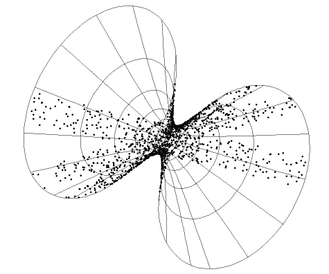 Figure 1
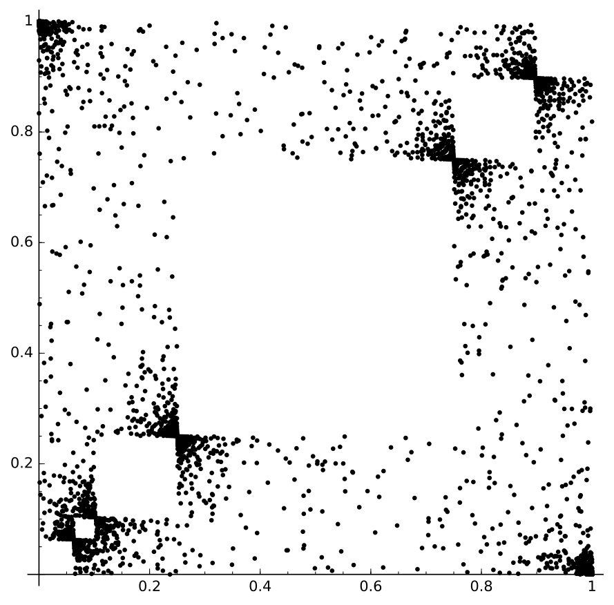 Figure 1
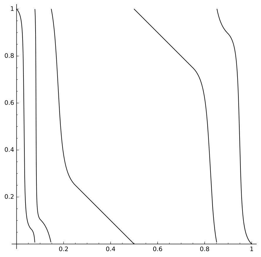 Figure 4
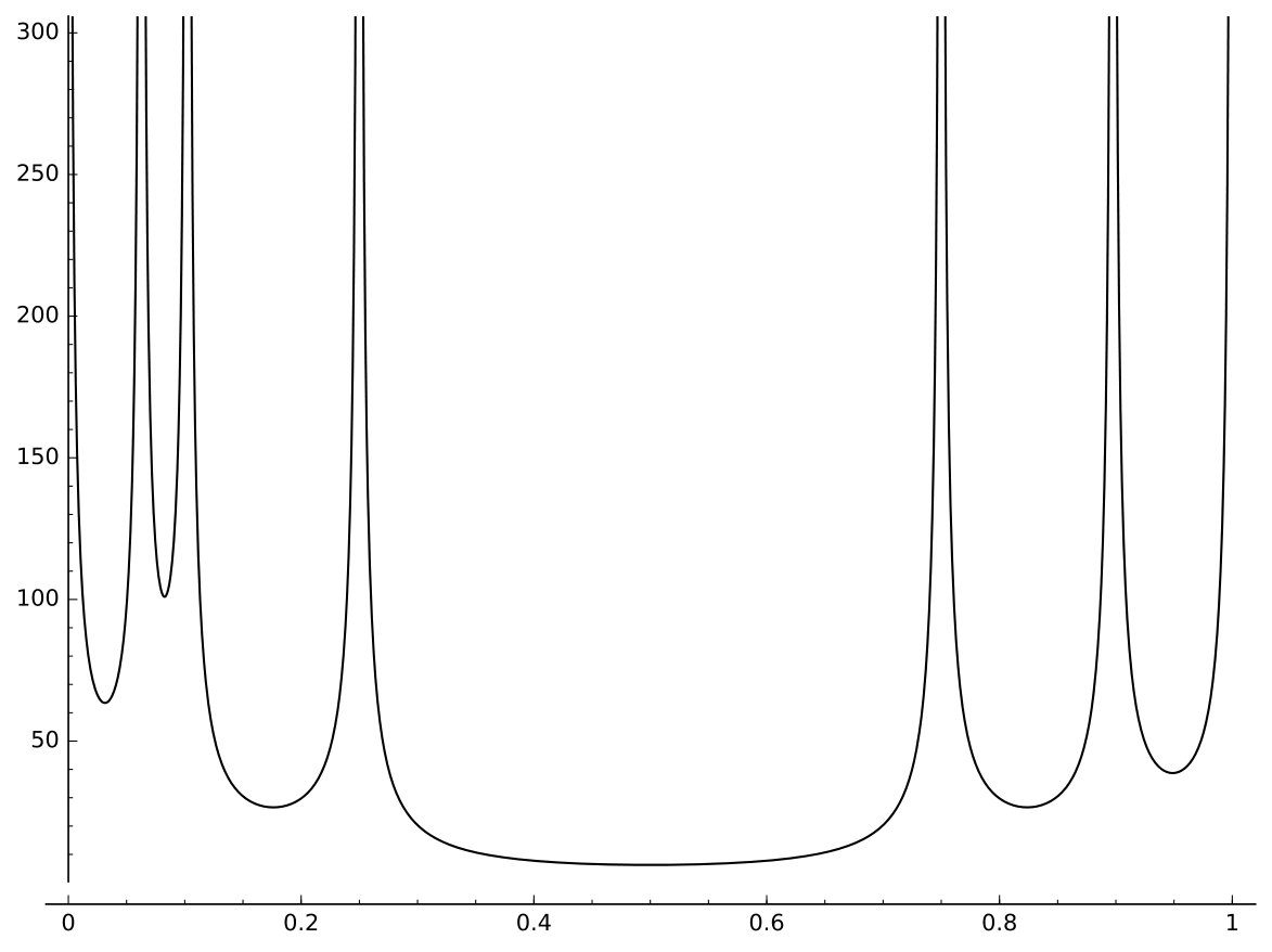 Figure 5
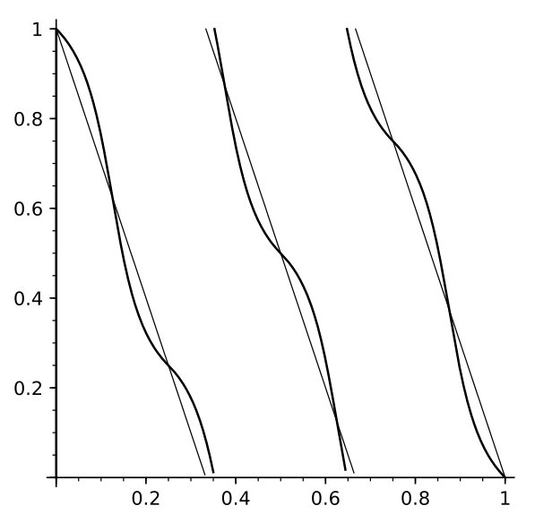 Figure 7
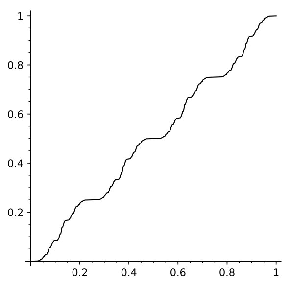 Figure 8
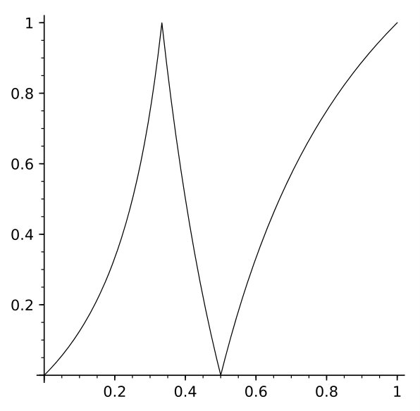 Figure 9
Peer Reviews
No public reviews on file for this paper yet. If you reviewed it on a platform where reviews are public (OpenReview, ICLR, NeurIPS, ICML), you can paste yours below so the community can read it here.
Videos
No videos yet. Explain this paper in a talk, walkthrough, or lecture? Add one.
Billiards on pythagorean triples
and their Minkowski functions
Giovanni Panti
Department of Mathematics, Computer Science and Physics
University of Udine
via delle Scienze 206
33100 Udine, Italy
Abstract.
It has long been known that the set of primitive pythagorean triples can be enumerated by descending certain ternary trees. We unify these treatments by considering hyperbolic billiard tables in the Poincaré disk model. Our tables have ideal vertices, and are subject to the restriction that reflections in the table walls are induced by matrices in the triangle group . The resulting billiard map acts on the de Sitter space , and has a natural factor on the unit circle, the pythagorean triples appearing as the -preimages of fixed points. We compute the invariant densities of these maps, and prove the Lagrange and Galois theorems: A complex number of unit modulus has a preperiodic (purely periodic) -orbit precisely when it is quadratic (and isolated from its conjugate by a billiard wall) over .
Each as above is a -to- orientation-reversing covering map of the circle, a property shared by the group character . We prove that there exists a homeomorphism , unique up to postcomposition with elements in a dihedral group, that conjugates with ; in particular —whose prototype is the classical Minkowski question mark function— establishes a bijection between the set of points of degree over and the torsion subgroup of the circle. We provide an explicit formula for , and prove that is singular and Hölder continuous with exponent divided by the maximal periodic mean free path in the associated billiard table.
2020 Math. Subj. Class.: 37D40; 11J70.
The author is partially supported by the research project SiDiA of the University of Udine.
1. Introduction
Rational points in the real projective line involve two integers, a numerator and a denominator; we can enumerate them by reversing the euclidean algorithm or —equivalently— taking inverse branches of continued fraction maps. Rational points in the unit circle involve three integers, the two legs and the hypotenuse of a pythagorean triangle. As the line and the circle can be mutually parametrized with preservation of rational points, the complexity of the enumeration is the same, and there is a line of work (starting from [6], and running through [4], [11], [3], [33], [15] and references therein) describing how pythagorean triples can be generated by descending trees.
Ascending the same trees amounts to iterating continued fraction maps, and in [42] Romik analyzes one such map, relating it to the geodesic flow on the three-punctured sphere. It turns out that Romik’s map can also be seen as the Gauss map of even continued fractions; see [2, §4], [15, §5], [7, §2] for various developments.
Although there is a birational bijection with rational coefficients between the line and the circle, continued fraction maps on the two spaces are not exactly the same thing. Indeed, the rational symmetry group of the projective line is the extended modular group , while that of the circle is , the stabilizer of the Lorentz form inside . When embedded in a larger ambient group —say — they appear as the and the extended triangle groups, and neither is a subgroup of the other (of course, they are commensurable).
In this paper we develop continued fraction maps (of the “slow” type, that is with parabolic fixed points) directly on the circle, as factors of billiard maps determined by ideal polygons in the hyperbolic plane. We summarize our main results as follows:
- •
Let be a polygon in the Poincaré disk having vertices, all at the boundary at infinity . Let be the map that sends the interval between two vertices to the union of the remaining intervals via reflection in the corresponding polygon side. Let be the group character . Then and are conjugate by an essentially unique homeomorphism , which provides a bijection between the set of points of degree at most over and the torsion subgroup of . The homeomorphism is singular and Hölder continuous, of exponent divided by the maximal mean free path (see Definition 10.3) of periodic trajectories in the hyperbolic billiard determined by .
The route leading to the above statement is somehow long; we offer two justifications.
- (1)
The end result is a flexible and applicable tool. Indeed, the maximal mean free path referred to above equals twice the logarithm of the joint spectral radius of the set of matrices expressing reflections in the billiard walls. When the vertices of determine a unimodular partition of (an arithmetical condition explained in §5), this joint spectral radius can often be explicitly computed; see Example 10.6. 2. (2)
Along that route we encounter fair landscapes.
We describe our route: in §2 we determine finite sets of reflections generating the orthogonal group and its subgroups and , the latter being the stabilizer of the upper sheet of the hyperboloid . Then, as a warmup, in §3 we review the construction of the Romik map using our formalism. In §4 we provide explicit -equivariant bijections between the homogeneous space , the de Sitter space , the space of oriented geodesics in the hyperbolic plane, and that of quadratic forms of discriminant . These correspondences are known, but since they appear scattered in the literature and some care is required to extend the acting group from the usual to the full , our brief self-contained treatment in Theorem 4.1 may have some value. In §5 we treat unimodular partitions of the circle; a reader not interested in arithmetical issues may safely skip Theorems 5.3 and 5.5.
The preliminaries being over, we introduce in §6 our continued fraction maps as factors of billiard maps associated to ideal polygons whose vertices form a unimodular partition of the circle. Reflections in the table walls are expressed by elements of —which we naturally take as matrices— in the Poincaré model, and by matrices in in the Klein model. Here the de Sitter space plays a twofold rôle, as the phase space of as well as the space of shrinking intervals, this double nature being reflected in a double action of ; see Remark 5.2. In §7 we use the bijections in §4 to characterize the natural extension and the absolutely continuous invariant measure of . In §8 we show that the map and the extended fuchsian group generated by are orbit-equivalent, and prove the following statement, which combines the classical Lagrange and Galois theorems. A complex number of unit modulus is quadratic over if and only if its -orbit is eventually periodic; moreover, if this is the case, then the conjugate point has the reverse period, and the two points are purely periodic precisely when they are separated by a billiard wall.
In §9 we introduce the conjugacy alluded to above. It is a natural conjugacy; indeed, is an -to- orientation-reversing covering map of the circle, a topological property shared by precisely one group character, namely . We thus have a “linearized” version of a continued fraction map, precisely as the tent map on is a linearized version of the Farey map. It turns out (Lemma 9.3) that the natural symbolic coding of points via , as well as the analogous coding via , characterizes the ternary betweenness relation on the circle. Since the latter relation determines the circle topology, we obtain in Theorem 9.2 that and are conjugate by a homeomorphism , unique up to postcomposition with elements of the dihedral group with elements. This homeomorphism is the analogue of the classical Minkowski question mark function [19], [43], [27], which conjugates the Farey map with the tent map. We provide in Theorem 9.4 an explicit expression for analogous to the Denjoy-Salem formula [43, p. 436] for the question mark function, and show in Examples 8.4 and 9.5 how the arithmetic properties of and are intertwined by . In Theorem 10.1 we provide an ergodic-theoretic proof of the fact that has zero derivative at Lebesgue-all points.
In the final Theorem 10.5 we complete the proof of the connection sketched above between the joint spectral radius of and the Hölder exponent of . In all instances we examined the Lagarias-Wang finiteness conjecture ([31], see §10) turned out to be true for , and a maximizing periodic billiard trajectory was easily guessed and verified. It is plausible that the conjecture holds for all billiard tables determined by unimodular partitions of the circle, and we leave this as an interesting open problem.
2. Notation and preliminaries
Since we treat various spaces of matrices, we will distinguish them notationally, by using boldface for matrices and lightface for ones. Points in are written in boldface and are always column vectors, although we may write for typographical reasons. We will use square or round brackets for vectors and matrices, according whether we are in a projective setting (that is, up to multiplication by nonzero scalars) or in a linear-algebra one. Zero entries in matrices are replaced by blank spaces.
Let
[TABLE]
be the matrix of the three-variable Lorentz quadratic form, and let be the corresponding symmetric bilinear map. The upper sheet of the -sheeted hyperboloid is one of the standard models of the hyperbolic plane, other models being the upper halfplane , the Klein disk , and the Poincaré disk ; we refer the reader to [10] for an enjoyable introduction to hyperbolic geometry. We need explicit bijections between these models, so we introduce a fifth auxiliary model, namely the upper hemisphere , and state a lemma.
Lemma 2.1**.**
The spaces , , , , are in bijective correspondence via the commuting diagram
[TABLE]
where
- •
* is the natural quotient map,*
- •
* is the stereographic projection through ,*
- •
,
- •
\upsilon([x_{1},x_{2},x_{3}])=\bigl{(}x_{1}/x_{3},x_{2}/x_{3},(x_{3}^{2}-x_{1}^{2}-x_{2}^{2})^{1/2}/x_{3}\bigr{)}* is the “vertical” projection,*
- •
* is the stereographic projection through to the halfplane , followed by the obvious identification of the latter with ,*
- •
* is the stereographic projection through to the disk , followed by the obvious identification of the latter with ,*
- •
* is the Möbius transformation induced by the Cayley matrix C=2^{-1/2}\bigl{[}\begin{smallmatrix}1&-i\\ -i&1\end{smallmatrix}\bigr{]}\in\operatorname{PSL}_{2}\mathbb{C} (as customary, we blur the distinction between matrices and the maps they induce).*
These correspondences extend to the respective ideal boundaries.
Proof.
The proof reduces to a commentary on the figure on page of [10]. The upper-left triangle commutes because sends to \bigl{(}x_{1},x_{2},(x_{3}^{2}-x_{1}^{2}-x_{2}^{2})^{1/2}\bigr{)}/x_{3}=(x_{1},x_{2},1)/x_{3}=(1/x_{3})(x_{1},x_{2},x_{3})+(1-1/x_{3})(0,0,-1). The upper-right triangle commutes because sends to . The lower-right triangle commutes because, given ,
[TABLE]
The fact that these correspondences extend to the ideal boundaries is obvious as soon as the boundary of and the maps , , on it are properly defined. We see as the intersection of the projective closure of (i.e., the variety in ) with the plane at infinity , and we set
[TABLE]
We can then view as the limit (in the euclidean metric of an appropriate local chart) of \bm{x}(t)=t\bigl{(}x_{1},x_{2},(x_{1}^{2}+x_{2}^{2}+1/t^{2})^{1/2}\bigr{)}\in\mathcal{L}, for . An easy computation shows that the -, -, -images of , as defined above, agree with the limits (in the euclidean metric) of , , , for . This guarantees the required commutativity. ∎
It is well known that the orthogonal group of the Lorentz form has four connected components, namely the component of the identity (which is a normal subgroup) and its cosets with respect to the diagonal matrices having diagonal entries , , . The union of the component of the identity with its -coset is the special orthogonal group , while its union with the -coset is the group of all matrices that preserve ; equivalently, \operatorname{O}_{2,1}^{\uparrow}\mathbb{R}=\{\bm{A}\in\operatorname{O}_{2,1}\mathbb{R}:\text{the (3,3)\bm{A}>0}\}. We will write for the component of the identity.
The group of isometries (including the orientation-reversing ones) of is , which acts on as follows: given A=\bigl{[}\begin{smallmatrix}a&b\\ c&d\end{smallmatrix}\bigr{]}, then equals if , and equals if . Conjugating with the Cayley matrix we obtain the group
[TABLE]
which acts on via
[TABLE]
We construct an isomorphic representation by identifying the vector with the matrix
[TABLE]
on which acts on the left by . This is a well defined action, independent from the lift of to , linear, and preserving the form . Computing the images of the -parameter subgroups in the Iwasawa decomposition of provides a geometric picture of the representation, namely
[TABLE]
Convention 2.2**.**
In order to simplify notation we adopt the convention that, whenever a matrix in is denoted by a certain capital letter, then its image under the above representation, and its -conjugate, are denoted by the same capital letter in bold and in calligraphic fonts, respectively. With this understanding, we give names to a few matrices that will recur throughout this paper.
[TABLE]
Explicit computation —which we omit— shows that on , for every in the above -parameter subgroups, and also for ; therefore the identity holds for every . The action of on descends to a projective action on that fixes the Klein model and its boundary . These observations, together with Lemma 2.1, imply that for every the diagram
[TABLE]
commutes. The analogous diagram involving the ideal boundaries of commutes as well, and actually simplifies. Indeed, the nontrivial bijection reduces on to the obvious identification , while reduces to the stereographic projection through , namely . We will thus switch freely between and , using as a neutral name for both.
Let be a polygon in , bounded by geodesics , and having angles at vertices , with integers or (if the corresponding vertex lies in ); the Gauss-Bonnet formula forces . The extended Coxeter group associated to is the subgroup of generated by the reflections in the sides of . It has the presentation
[TABLE]
(with the understanding that relators do not appear), and is a fundamental domain for it. Its index- subgroup of orientation-preserving elements is a fuchsian group of finite covolume; see [28], [32]. When is a triangle we write and for and , referring to them as a triangle group and an extended triangle group, respectively (the adjective extended stresses the fact that orientation-reversing isometries are allowed; in both cases, the action on is properly discontinuous). Note that the numbers determine the triangle up to isometry, and hence the groups up to conjugation. We will freely use all of the above terminology when working in other models of the hyperbolic plane.
Let us return to the Lorentz form . We recall that, given a nonisotropic vector , the reflection is the unique linear involution of that fixes pointwise the polar hyperplane and exchanges with . An easy computation (of course, all of this is well known) shows that:
- (i)
[TABLE]
- (ii)
preserves ,
- (iii)
in terms of matrices,
[TABLE]
- (iv)
if and only if .
Notation 2.3**.**
- •
(respectively, , , ) is the intersection of (respectively, , , ) with .
- •
\operatorname{PSL}^{\pm}_{2}\mathbb{Z}=\{A\in\operatorname{PSL}^{\pm}_{2}\mathbb{R}:\text{A\mathbb{Z}}\}.
- •
.
- •
(and analogously for other groups generated by involutions) is the group of all products of an even number of elements in .
The four matrices in (2.3) are in ; in particular they are of the form , for equal to , , , , respectively. In [35] it is proved that the five reflections , , , , generate (see [17] for an elementary proof which avoids the theory of Kac-Moody Lie algebras); we give an independent and expanded version in the following theorem.
Theorem 2.4**.**
We have , , , which is isomorphic to the extended triangle group ; adding as a further generator we obtain the full group . The group is an index- subgroup of , and equals ; its image inside is .
Proof.
We work in . Let ; then, by definition, is an arithmetic fuchsian group. We observe that is the triangle group . Indeed are the reflections in the three geodesics
- •
, whose endpoints are and ;
- •
, whose endpoints are and ;
- •
, whose endpoints are and .
These geodesics determine a triangle in with vertices at with angle , at with angle , and at the ideal point with angle [math].
Clearly is a subgroup of , and it is well-known that a fuchsian group containing a triangle group must itself be a triangle group [44, §6]. The partially ordered set of all nine non-cocompact arithmetic triangle groups has been determined by Takeuchi in [46], and is maximal in it; therefore . Adding as a further generator to we obtain , as claimed.
For the second statement, observe that replacing the generator with means replacing with the geodesic whose endpoints are [math] and . The polygon determined by is the triangle , with angles at , and [math] at and at ; hence is the extended triangle group . Clearly , and by computing
[TABLE]
we see that C^{-1}\bigl{(}\operatorname{PSU}^{\pm}_{1,1}\mathbb{Z}[i]\bigr{)}C is a subgroup of . Taking into account the respective fundamental domains, it is easy to check that has index in ; therefore C^{-1}\bigl{(}\operatorname{PSU}^{\pm}_{1,1}\mathbb{Z}[i]\bigr{)}C equals either or the full . However, this second possibility is ruled out by the fact that (which is the extended triangle group) contains elements of order , and hence of trace (up to sign), while clearly no element of may have trace . ∎
3. Pythagorean triples and the Romik map
A [primitive] pythagorean triple is a point such that , , and . Pythagorean triples correspond bijectively to rational points in the unit circle, which in turn correspond, via stereographic projection, to points in . These correspondences provide various techniques for enumerating triples, among which the one known to Euclid: given any reduced fraction , the triple is pythagorean, and every pythagorean triple is uniquely obtainable in this way (the gcd in the denominator is if , and otherwise). As noted in the introduction, many techniques are cast in the form of the descent of a binary or ternary tree.
A remarkable connection with the theory of continued fractions is offered in [42]; as a warmup, we sketch it using our notation. We partition in four quarters , with . Let . Then acts on (viewed as , see the diagram (2.4) and the resulting identifications) by exchanging with the other point of intersection of with the line through and ; the interval is thus bijectively mapped to the union of the other three intervals. We fold back to via the reflection acting on , the rotation on , and the reflection on ; see Figure 1. Conjugating this process via the stereographic projection through we obtain the Romik map in Figure 2. By construction, it is a continuous piecewise-projective selfmap of the real unit interval . It is composed of three pieces, each one mapping bijectively a subinterval of to the whole interval. The computation of these pieces is built-in in our formalism: indeed, since stereographic projection from is on , computation amounts to switching from boldface to lightface. Thus, the first piece is induced by J(FPF)=\bigl{[}\begin{smallmatrix}1&\\ -2&1\end{smallmatrix}\bigr{]} acting on , the second one by (JF)(FPF)=JPF=\bigl{[}\begin{smallmatrix}-2&1\\ 1&\end{smallmatrix}\bigr{]} acting on , and the third by F(FPF)=PF=\bigl{[}\begin{smallmatrix}2&-1\\ 1&\end{smallmatrix}\bigr{]} on .
We adopt another notational shorthand, by consistently writing (or , ) for pairs , , identified as in the discussion following the diagram (2.4). We recall that the residue field of the point in the projective variety is . If we say that is a rational point; in this case has a canonical presentation as a pythagorean triple. The corresponding has a canonical presentation as well, but a subtler one. For each prime integer , write uniquely , for integers , and let (corresponding, as in Euclid’s setting, to ). It is well known —and easy to prove [20]— that every factors uniquely in as a product of a unit in and finitely many numbers and their inverses. This implies that the set of primitive pythagorean triples forms a multiplicative group, isomorphic to the direct sum of the cyclic group of order with countably many copies of the infinite cyclic group. We thus obtain our second canonical presentation: every can be uniquely expressed as , with and having prime decomposition of the form
[TABLE]
with , for every , and the pairs all distinct.
4. The de Sitter space
The de Sitter space is the one-sheeted hyperboloid ; it is a lorentzian manifold of constant positive curvature [37], [36]. The de Sitter space is in natural bijection with various spaces of interest to us: these bijections are well known, albeit a bit scattered in the literature. We collect the relevant facts in Theorem 4.1, whose nonstandard feature is the rôle of as the acting group, instead of the usual .
We recall from §2 that is a group isomorphism from to . We define now another isomorphism by . In the following theorem we let have value [math] on , and on ; also, we denote any group action by a star.
Theorem 4.1**.**
The spaces in the following list, together with the specified base points and transitive left actions of , are in bijective correspondence. These correspondences preserve the base points and are equivariant with respect to the actions.
- (S1)
The de Sitter space , with base point and action .
- (S2)
The coset space , for the subgroup of diagonal matrices, with base point and action .
- (S3)
, with base point and action .
- (S4)
, with base point and action .
- (S5)
The space of oriented geodesics in , with base point the geodesic from to and action .
- (S6)
The space of quadratic forms q\bigl{(}\begin{smallmatrix}x\\ y\end{smallmatrix}\bigr{)}=q_{1}x^{2}-q_{2}xy+q_{3}y^{2} of discriminant , with base point and action (A*q)\bigl{(}\begin{smallmatrix}x\\ y\end{smallmatrix}\bigr{)}=(\det A)q\bigl{(}A^{-1}\bigl{(}\begin{smallmatrix}x\\ y\end{smallmatrix}\bigr{)}\bigr{)}.
Each space carries a -invariant infinite measure, which is the quotient Haar measure in (S2), and is induced by the form in (S3). In (S1), the measure of a Borel subset of is the euclidean volume of the cone , and analogously for (S6).
Proof.
The natural bijections among the spaces in (S3), (S4), (S5) are the obvious ones resulting from the diagram (2.4). Here we will first describe the bijections among (S2), (S3), (S6), and then the one between (S1) and (S6).
Let be a form as in (S6), associated to the symmetric matrix
[TABLE]
of determinant . We obtain a pair as in (S3) by labeling the two roots of as follows:
- (a)
if and , then and ;
- (b)
if and , then and ;
- (c)
if , then
[TABLE]
Given a pair as in (S3), we set
[TABLE]
thus defining a coset as in (S2).
Finally, any in (S2) determines a symmetric matrix of determinant via
[TABLE]
note that is well defined, i.e., independent from the choice of a representative in and from the lift of this representative to .
It is clear that each of these constructions preserves the base points and is equivariant with respect to the listed actions. Therefore, the claimed correspondence between (S2), (S3), (S6) follows as soon as we prove that the final equals the starting . We check case (c), leaving the simpler cases (a) and (b) to the reader. By definition,
[TABLE]
so that
[TABLE]
Hence
[TABLE]
which is the initial ; note the use of the identity J^{\pm 1}\bigl{(}\begin{smallmatrix}&1\\ 1&\end{smallmatrix}\bigr{)}J^{\pm 1}=\pm 1\bigl{(}\begin{smallmatrix}&1\\ 1&\end{smallmatrix}\bigr{)} in the computation.
The bijection between (S1) and (S6) is a simple change of variables, namely
[TABLE]
This change of variables transforms the matrix in (4.1) to , where is the matrix in (2.1). This implies that the bijection is equivariant with respect to the actions listed in (S1) and (S6); see also Remark 5.2.
The statement about invariant measures is well known; see, e.g., [22, §8]. ∎
For future reference we list here the form and the point as a function of :
[TABLE]
5. Circle intervals
The unit circle is cyclically ordered by the ternary betweenness relation , which reads “ are pairwise distinct, and traveling from to counterclockwise we meet ”. Every pair of distinct points determines two closed intervals, namely and . Given in the de Sitter space, the set is an interval as well (the factor , i.e., the third coordinate of , makes the definition independent from the choice of a representative for ). Let us denote the ordinary cross product of two vectors in by .
Lemma 5.1**.**
Let be distinct, and let
[TABLE]
the right-hand side being independent from the chosen lifts of to . Then the following statements hold.
- (i)
, and .
- (ii)
Let be the pair corresponding to according to Theorem 4.1. Then we have
[TABLE]
- (iii)
For every , we have , which equals if , and otherwise.
- (iv)
* if and only if both and are rational points.*
- (v)
The arclength of and the third coordinate of are related by .
- (vi)
If and do not lie on the same diameter (i.e., by (v), if ), then the unique circle in perpendicular to and passing through has center and curvature .
- (vii)
Assume that
[TABLE]
with arclength tending to [math] (i.e., ). Then \lim_{t\to\infty}\operatorname{arclength}(I_{\bm{w}_{t}})\big{/}(2/w_{t,3})=1.
Proof.
(i) Every rotation
[TABLE]
leaves invariant the arclength of and the third coordinate of (because belongs to as well as to , and hence (\bm{L}\bm{S}\bm{t}^{\prime}\times\bm{L}\bm{S}\bm{t})\big{/}\langle\bm{S}\bm{t}^{\prime},\bm{S}\bm{t}\rangle=\bm{S}\bm{w}). Therefore we assume without loss of generality and , for some . Then, by explicit computation, \bm{w}=\bigl{(}(\sin r)\big{/}(1-\cos r),1,(\sin r)\big{/}(1-\cos r)\bigr{)}, which is indeed in . Let , and let . Then, by elementary projective geometry, takes value [math] in precisely two points, namely in and in the unique solution to . Again by explicit computation, has derivative , which is positive at [math]. This, and extending to be periodic, then implies that if and only if , as claimed.
(ii) We have , and analogously for . Our statement amounts then to the verification that the vector
[TABLE]
resulting from (5.1) equals the vector given by (4.4). This is a straightforward computation.
(iii) Let be a point in , and choose a representative for it with positive third coordinate. Then, for every , the third coordinate of is still positive; we thus have iff iff iff iff . The second statement follows from the first and the remark that is equivalent to if , and to if .
(iv) The right-to-left implication follows from the definition of . Conversely, if then the proof of the equivalence between (S1) and (S6) in Theorem 4.1 yields that the form corresponding to has rational coefficients. Since has discriminant , the roots of (given by (a), (b), (c) in the proof of the same Theorem 4.1) are rational numbers. By (ii), and are the reverse stereographic projections through of these roots, and thus are rational points.
(v) As in (i), we assume and . Then, as computed in (i), w_{3}=(\sin r)\big{/}(1-\cos r)=\cot(r/2), and our statement follows.
(vi) Looking at as a point in , the identities mean that is the intersection point of the two lines tangent to at and ; thus the described circle has center . Upon applying the rotation in the proof of (i), the statement about the curvature follows by direct inspection.
(vii) This is clear. ∎
Remark 5.2**.**
Since, as it is easily seen, the map is a bijection between and the space of closed circle intervals, it is tempting to add a seventh item to the list in Theorem 4.1. However this would not be correct, since the action in Lemma 5.1(iii) does not agree with the one in Theorem 4.1(S1). In other words, acts on the space of intervals via the “bold” isomorphism , while it acts on the de Sitter space via . The following commuting diagram may clarify the situation
[TABLE]
In (5.2), the rightmost vertical arrow is the involutive automorphism of , which restricts to the isomorphisms and . Since these isomorphisms obviously preserve the fact that a matrix has integer entries, Theorem 2.4 implies that \operatorname{SO}_{2,1}\mathbb{Z}=\Lambda\bigl{[}\langle F,P,G\rangle\bigr{]}=\langle-\bm{F},-\bm{P},-\bm{G}\rangle\simeq\Delta^{\pm}(2,4,\infty) and \operatorname{SO}^{\uparrow}_{2,1}\mathbb{Z}=\Lambda\bigl{[}\langle F,P,G\rangle^{+}\bigr{]}=\langle\bm{F},\bm{P},\bm{G}\rangle^{+}\simeq\Delta(2,4,\infty).
When working with continued fractions algorithms one naturally deals with unimodular intervals in , namely intervals with rational endpoints and such that \det\bigl{(}\begin{smallmatrix}p&p^{\prime}\\ q&q^{\prime}\end{smallmatrix}\bigr{)}=-1; for example, the intervals of continuity for the Gauss map are unimodular. It is a trivial —but key— fact that the modular group acts simply transitively on such intervals. The situation for intervals on the circle is more involved.
Theorem 5.3**.**
The set is partitioned in two orbits, corresponding to the parity of , by the action of . On each orbit the action is simply transitive. Replacing with its index- subgroup \Lambda\bigl{[}\langle F,P,J\rangle^{+}\bigr{]} each orbit is further split in two.
Proof.
It is easy to check that each of , , preserves the parity of ; hence there are at least two orbits.
Choose and let be the corresponding ordered pair according to Theorem 4.1. An appropriate power of the parabolic matrix (that fixes ) sends to a new pair with . By [42, Theorem 2(i)], the orbit of under the Romik map ends up after finitely many steps, say the th step, in one of the two parabolic fixed points [math], . For each , let
[TABLE]
be the matrix acting at time . Then , and is such that . Postcomposing , if necessary, with (if ) or with (if ), we have .
Suppose . Then because the point corresponding to equals by (4.4), and also equals , which is a point in . This implies that an appropriate power of the parabolic matrix PJ=\bigl{[}\begin{smallmatrix}1&2\\ &1\end{smallmatrix}\bigr{]} maps either to or to . If, on the other hand, , then the same argument with replaced by (JPJ)F=\bigl{[}\begin{smallmatrix}2&1\\ -1&\end{smallmatrix}\bigr{]} (which is parabolic fixing ) yields that a power of maps either to or to .
Summing up, we have proved that the pair is in the -orbit of one of the pairs . Now, the rotation maps the first pair to the third, and the second to the fourth. By Theorem 4.1 this means that the original point is in the \Lambda\bigl{[}\langle F,P,G\rangle^{+}\bigr{]}-orbit of either or of . Since \Lambda\bigl{[}\langle F,P,G\rangle^{+}\bigr{]}=\operatorname{SO}^{\uparrow}_{2,1}\mathbb{Z} by Remark 5.2, our first claim is established.
Simple transitivity follows from the fact that both and have trivial stabilizer in (because an element of a fuchsian group that fixes two distinct cusps must be the identity).
Finally, the pairs remain distinct modulo . Indeed, the latter is the triangle group , which has two distinct cusp orbits, and it is easy to check that any identification of the above four pairs would collapse these two orbits. ∎
We can now define unimodularity for circle intervals.
Definition 5.4**.**
Let be distinct rational points in , and let be the point corresponding to according to Lemma 5.1. If and is even (odd), then we say that is an even (odd) unimodular interval.
Theorem 5.5**.**
Let be as in Definition 5.4; then the following conditions are equivalent.
- (1)
* is unimodular (either even or odd).* 2. (2)
* has integer entries.* 3. (3)
* is the image either of \bigl{[}[0,-1,1],[0,1,1]\bigr{]} or of \bigl{[}[1,0,1],[0,1,1]\bigr{]} under some (necessarily unique) element of .* 4. (4)
* (here are the canonical presentations of as primitive pythagorean triples).*
If these conditions hold, then is odd iff it is the image of \bigl{[}[1,0,1],[0,1,1]\bigr{]} iff . Moreover, belongs to , and the matrix corresponding to it under Convention 2.2 is
[TABLE]
where are identified with as in §3.
Proof.
(1) (2) Since , this is immediate from the explicit formula for in (2.6).
(2) (3) Let
[TABLE]
(see Lemma 5.1(ii)). Then, as in the proof of Theorem 5.3, we construct such that equals either or . Since , there exists with , for some . Hence, . We then have
[TABLE]
and the leftmost entry in the display is a matrix with integer entries. Multiplying through by , subtracting the identity matrix , and multiplying by on the right, we see that the matrix
[TABLE]
must have integer entries. This implies that the denominator of the rational number must divide , and so must do the denominator of ; therefore is an integer. Thus, as in the proof of Theorem 5.3, an appropriate power will map either to or to ; therefore, \Lambda\bigl{(}(PJ)^{k}B\bigr{)}\bm{w}\in\{(1,0,0),(1,1,1)\}. Now, , and equals the “bold” isomorphism on , with range . Thus is the image either of or of under some element of , a statement equivalent to (3) by Remark 5.2.
(3) (4) This is clear, since and .
(4) (1) If , then by the definition of in Lemma 5.1; assume then . In every pythagorean triple one of the legs must be even, and the other leg and the hypotenuse both odd. The condition forces to be both even and both odd (or conversely). Since are surely both odd, all the entries in must be even; thus .
The stated characterization of being even/odd is clear from the previous proof.
By Theorem 5.3, is in the -orbit of one of , , , . Hence is a conjugate either of , or of , or of , or of by a matrix in ; in any case, it belongs to .
Finally, let be the matrix in (5.3). By direct computation
[TABLE]
which has the form \bigl{[}\begin{smallmatrix}\alpha&\beta\\ \bar{\beta}&\bar{\alpha}\end{smallmatrix}\bigr{]}, as can easily be checked; hence . If we can prove that has entries in , then necessarily . Indeed, the matrix would then belong to the fuchsian group , and would fix the two cusps ; hence, it must be the identity matrix.
Write uniquely , , as explained in §3. By Theorem 5.3, there exists such that
[TABLE]
This implies that the determinant divides in . Since
[TABLE]
we have
[TABLE]
which has entries in . ∎
6. Billiard maps
Having arranged our tools in working order, we proceed to our core objects.
Definition 6.1**.**
A unimodular partition of the unit circle is a counterclockwise cyclically ordered -uple of pythagorean triples, of cardinality at least , such that each interval is unimodular (including ; here and in the following we are writing indices modulo ). We will write for the points defined by Lemma 5.1.
According to our conventions, and without further notice, we will often switch to a complex-numbers setting, thus writing for .
For every , let be the geodesic in of ideal endpoints and ; of the two halfplanes determined by , let be the one containing all other , for . Then is a polygon with sides and ideal vertices , on which we can play billiards in the usual way. Namely, any unit velocity vector attached to an infinitesimal ball in the interior of determines an oriented geodesic starting from an ideal point and ending at . The ball travels along at unit speed, until it hits the side determined by the half-open interval to which belongs (unless is one of the vertices, in which case the ball is lost at infinity). When hitting , the ball rebounces with angle of reflection equal to the angle of incidence, and continues its trajectory along the geodesic which is the image of with respect to the reflection with mirror . This reflection is induced by the matrix in (5.3) (with and ), and thus has ideal initial and terminal points and , respectively. All of this naturally suggests the following standard definition [18, Chapter 6], [16, §IV.1].
Definition 6.2**.**
The billiard map determined by the unimodular partition is the map from to itself defined by , where is the index of the unique half-open interval containing , and . The map is continuous, and determines a topological dynamical system. We denote by the factor system naturally induced by the projection ; in short, for .
We will freely use Theorem 4.1 to conjugate to a map acting on any of the spaces (S1)–(S6); we will still denote the conjugated map by , slightly abusing notation. For ease of visualization (and crucially in §9 and §10) we will also conjugate and to maps on and , respectively; these last conjugations are realized through the normalized (i.e., the image is divided by ) argument function .
Example 6.3**.**
The ordered -uple
[TABLE]
is a unimodular partition, whose corresponding billiard table is shown in Figure 3 (left). The matrices are
[TABLE]
The graph of the -conjugate of is shown in Figure 3 (right); it requires caution in two respects. First, is a continuous map on and, second, it is piecewise-defined via six pieces, whose endpoints are given by the six -fixed points ( included). We plot in Figure 4 (left) points of the -orbit of a “typical” point in the de Sitter space , and in Figure 4 (right) their -images. The cluster points apparent in this latter figure correspond to the six fixed points cited above. These are indifferent fixed points (i.e., the derivative of has absolute value ), and this forces the unique -invariant measure absolutely continuous with respect to the Lebesgue measure to be infinite; see Theorem 7.2 and Figure 5. Note that is not injective: the points and are different, but both get mapped to (see however Theorem 7.1(i)).
We let be the group generated by , and the associated fuchsian group. By conjugating with an appropriate element of we always assume, without loss of generality, that . As noted in §2, admits the presentation , and hence is isomorphic to the free product of copies of the group of order two. Equivalently stated, each element of can be uniquely written as a word in the generators , subject to the only condition that the same generator does not appear in two consecutive positions. Since has finite hyperbolic area, and have finite index in .
Definition 6.4**.**
Let be as in Definition 6.2. For each , let be determined by ; the point in the Cantor space is the -symbolic sequence of .
Lemma 6.5**.**
The -symbolic-sequence map is injective. Its range is the set of all sequences such that:
- (i)
if for some , then for every ;
- (ii)
for any , the tail of is neither of the form , nor of the form (the bar denoting periodicity).
Remark 6.6**.**
Since we are considering half-open intervals, each has precisely one -symbolic sequence; thus is well defined. This differs slightly form other treatments of Gauss-like maps (see, e.g., [29, §2.1] or [45, §1.2.1]), in which rational points have two symbolic sequences. Note that is not continuous; indeed, if it were it would have compact image, which is not the case (e.g., all sequences of the form lie in the image, but the resulting sequence of sequences does not have a limit point in ).
Proof of Lemma 6.5.
Each is an involution, and exchanges with , the bar denoting topological closure. However, in this proof we carefully distinguish (which maps bijectively to ) from (which is one of the branches of , the one that maps bijectively to ). We do so in order to prepare the ground for the proof of Theorem 9.2, where the argument we are going to provide will be adapted to another -to- covering map of .
Let . If , then . Since is a -fixed point, we have for every . Moreover, if and , then we have , which implies , because . Hence cannot have tail . The fact that cannot have tail is proved in [12, Theorem 2.1]. We conclude that every -symbolic sequence must satisfy (i) and (ii).
Conversely, we fix satisfying (i) and (ii) and show that there exists a unique point having as -symbolic sequence. We need a preliminary remark: suppose we know that is the unique point having -symbolic sequence . Then, by direct inspection, we have:
- (a)
if is in the interior of and , then is in the interior of and is the unique point having -symbolic sequence ;
- (b)
the same conclusion holds if , provided that .
Case 1. The sequence has tail , say from time on. If , then there exists a unique point having -symbolic sequence , namely . If , then the previous remark and induction show that is the only point having -symbolic sequence .
Case 2. The sequence does not have tail , for any . Since for every , we have strict inclusions for every , and hence a strictly decreasing sequence of nested intervals
[TABLE]
We claim that this sequence shrinks to a singleton. Indeed, each set in (6.1) is a unimodular interval, strictly containing the following one. By Lemma 5.1(v) the third coordinates of the corresponding points on the de Sitter space form a strictly increasing sequence. Since we are dealing with unimodular intervals, these third coordinates are integer numbers, and a strictly increasing sequence of integers must go to infinity. Therefore the arclengths of the intervals go to [math], and the intersection of the sequence in (6.1) contains at least one point —by compactness— but no more than one.
Let be the shrinking point of (6.1) and let ; we prove by induction (note that, clearly, no point other than may have -symbolic sequence ). We have ; if were different from , then necessarily and . Therefore, for every we have \sigma=B^{t}(\sigma)\in B^{t}[\mathscr{A}_{a_{0}}\cdots\mathscr{A}_{a_{t-1}}\bigl{[}\overline{I}_{a_{t}}]\bigr{]}=\overline{I}_{a_{t}}, and thus belongs to . This implies , which contradicts (ii); hence . For the inductive step, assume for . Then has -symbolic sequence and is the unique shrinking point of the chain
[TABLE]
Applying the base step above to we get . ∎
7. Natural extension and invariant measures
If has constant tail for some , i.e., for some , we say that is -terminating. If has periodic tail with minimal preperiod and period , we say that is -periodic or -preperiodic, according whether is [math] or greater than [math].
We will push the identification of the de Sitter space with a bit further by using the symbol for both; this is unambiguous since writing or clearly distinguishes the two uses. With this understanding, we denote by the set of all pairs such that:
- (i)
both and are -nonterminating;
- (ii)
and belong to different intervals.
For the map of Example 6.3, the orbit in Figure 4 is dense in .
Theorem 7.1**.**
The following facts hold.
- (i)
* is a bijection on .*
- (ii)
If is such that both and are -nonterminating, then for some .
- (iii)
Let be the -invariant measure on given by Theorem 4.1. Then is a measure-preserving system, and so is its factor , where is the pushforward measure induced by the projection .
- (iv)
The invertible system is the natural extension of .
Proof.
(i) The fact that maps into itself is clear. Writing for the involution of , it is also clear that on . In terms of symbolic sequences, all of this just amounts to and .
(ii) Let be both -nonterminating. By Lemma 6.5 there exists such that and belong to different intervals. By the definitions of and of , we have .
(iii) Any measurable is the disjoint union , where . Thus and, as \tilde{\mu}\bigl{(}\mathscr{A}_{a}[M_{a}]\bigr{)}=\tilde{\mu}(M_{a}), we have .
(iv) The set \{\sigma\in S^{1}:\text{\sigmaB-terminating}\} is clearly -invariant and has -measure [math]; modulo this nullset and its -counterimage, we have the commuting square
[TABLE]
By the very definition of the natural extension [41, p. 22], the metric system is the natural extension of its factor if the supremum of the family of measurable partitions
[TABLE]
is —modulo nullsets— the partition of in singletons. This condition amounts to the request that if , then there exists such that \pi\bigl{(}\widetilde{B}^{-t}(\sigma,\rho)\bigr{)}\not=\pi\bigl{(}\widetilde{B}^{-t}(\sigma^{\prime},\rho^{\prime})\bigr{)}. This request is clearly satisfied: if we take , while if we take , there is the least nonnegative integer such that and lie in different intervals. ∎
As usual in the context of Gauss-like maps, once a model of the natural extension has been determined the computation of the (unique) absolutely continuous -invariant measure is easy; we state the result for the -conjugates of and .
Theorem 7.2**.**
Let and write —abusing language— and for and , respectively. For , let , and let be the function defined by
[TABLE]
on , and having value [math] elsewhere. Then the following facts hold.
- (i)
The unique (up to constants) -invariant measure on absolutely continuous with respect to the Lebesgue measure is \,\mathrm{d}\tilde{\mu}=\pi^{2}\bigl{(}\sin(\pi(x-y))\bigr{)}^{-2}\,\mathrm{d}x\,\mathrm{d}y.
- (ii)
The unique (up to constants) -invariant measure on absolutely continuous with respect to the Lebesgue measure is \,\mathrm{d}\mu=\bigl{(}\sum_{a}h_{a}\bigr{)}\,\mathrm{d}x.
- (iii)
Both systems , are ergodic and conservative.
Proof.
(i) This is just a change of variables, easily performed in two steps. Let be defined by
[TABLE]
Then is a bijection from to ; indeed, it amounts to the componentwise application of , with the Cayley matrix. This implies that the pushforward of the infinite invariant measure of Theorem 4.1 via is (F_{2}\circ F_{1})^{*}\bigl{(}(\omega-\alpha)^{-2}\,\mathrm{d}\omega\,\mathrm{d}\alpha\bigr{)}. One now computes
[TABLE]
(ii) Let . Then is the integral
[TABLE]
of the invariant density in (i) along the fiber \{x\}\times\bigl{(}[0,x_{a}]\cup[x_{a+1},1]\bigr{)}.
(iii) It is easy to check that satisfies Thaler’s conditions [47, p. 69(1)–(4)]. This implies that is ergodic and conservative; therefore so is and its natural extension [1, Theorem 3.1.7]. ∎
We draw in Figure 5 the invariant density for the map of Example 6.3. We note that, in case , a direct geometric proof of Theorem 7.2(ii) was given by Kołodziej and Misiurewicz, using Ptolemy’s theorem on quadrilaterals inscribed in a circle [30], [34].
8. The Lagrange theorem
Our next result is a version of Serret’s theorem (two real numbers have the same tail in their continued fraction expansion precisely when they are -equivalent [24, §10.11], [39]) in modern language.
Theorem 8.1**.**
The map and the group are orbit equivalent. More precisely, given , there exists such that if and only if there exist such that . In particular, if belongs to then it is -terminating, its orbit landing in the unique vertex of which is -equivalent to .
Proof.
We begin proving the last assertion, for which the setting is expedient. Let then be a rational point, and let be the third coordinates of the points of Definition 6.1. We need a preliminary step.
Claim
By conjugating by an appropriate element of , we may assume that are all greater than [math], with at most one exception that may equal [math].
Proof of Claim
By Lemma 5.1(v), the greater is the arclength of , the smaller is , with corresponding to arclength . This implies that no more than one of the above third coordinates may be negative or [math]. Say that . If is even, then by Theorem 5.3 we may conjugate by the matrix in that sends to , and we are through. If is odd, than we conjugate by the matrix that sends to ; the image of will then have arclength . One of the new third coordinates may now have value [math], but none may have value or less, since value already corresponds to an arclength of , and the sum of the arclengths would exceed .
Having proved our claim we perform, if needed, this preliminary conjugation, which does not affect the validity of our statement; renaming indices, we assume and . If is one of , we are through. Otherwise, is in the interior of precisely one interval, say ; let . Then, lifting and to their canonical representatives (i.e., to pythagorean triples), we have the identity in
[TABLE]
Now, since , and since is in the interior of . This implies that the third coordinate of is strictly less than the third coordinate of , unless and , in which case we have equality. But the third coordinates of and are positive integers, and the exceptional case of equality is always preceded and followed by nonexceptional cases. Hence the process must stop, and this may happen only when the -orbit of lands in one of the interval endpoints .
For the first assertion, the “if” implication is clear. Assume . If one of is in then so is the other, and by the first part of the proof both and land in one of . Since the vertices of are -inequivalent, they must land in the same . Let then and . As noted in §6, factors uniquely as , for certain . Let be minimum such that . Then
[TABLE]
By (a) in the proof of Lemma 6.5, , and . ∎
The bijection between and rational points in extends to higher degrees.
Lemma 8.2**.**
Let correspond to as usual, and let . Then and . If is Galois totally real, then the Galois groups and are naturally isomorphic. In particular, assume that is quadratic over and let be its Galois conjugate. Then and is the Galois conjugate of with respect to the quadratic extension .
Proof.
Since the stereographic projection through is a rational map with rational coefficients, the identity holds (with the convention that ). All statements follow from elementary Galois theory, as soon as one realizes that . In this identity the left-to-right containment is obvious, and the other one follows from . ∎
The question of the validity of Lagrange’s theorem (preperiodic points correspond to quadratic irrationals) for the Romik map is left open in [42, §5.1]. It can be settled in the affirmative by the result in [38]; see also [14] for this issue, and [13] for diophantine approximation aspects of the Romik map. Here we provide a different proof, valid not only for the Romik map but for all maps based on unimodular partitions. Note that our proof covers not only Lagrange’s, but Galois’s theorem [40, Chapter III]: periodic points correspond to reduced irrationals.
Theorem 8.3**.**
The point is -preperiodic if and only if it is quadratic over . If this is the case and is the -symbolic sequence of (with the minimal period and the minimal preperiod, so that ), then the -symbolic sequence of the Galois conjugate is . In particular, the preperiodic is periodic iff so is iff .
Proof.
Let be -preperiodic. Clearly, for every , we have ; we can then assume that is -periodic, with -symbolic sequence . Let . By looking at the decreasing sequence (6.1) in the proof of Lemma 6.5, we obtain
[TABLE]
Since is also in the above intersection, it equals , and this yields a quadratic polynomial with coefficients in and having as root. This polynomial is not the zero polynomial, as is not the identity matrix, and is irreducible over because is -nonterminating and Theorem 8.1 applies.
Conversely, let be quadratic over . By Lemma 8.2 the conjugate is in as well. For , let , and let be the oriented geodesic of origin and endpoint . By Theorem 7.1 there exists such that, for , the points and belong to the same interval (so that does not cut the billiard table ), while cuts for every . In particular, the -symbolic sequences of and agree up to time included, and disagree at time . Let , ; since and are still conjugate in , by Lemma 8.2 and are conjugate in . Let be the coefficient ring of the module [8, Chapter 2 §2.2]. Then is an order in with fundamental unit , and thus the matrix
[TABLE]
(where is the conjugate of ) is in .
Now, \langle F,P,J\rangle=C^{-1}\bigl{(}\operatorname{PSU}^{\pm}_{1,1}\mathbb{Z}[i]\bigr{)}C is an index- subgroup of (see the end of the proof of Theorem 2.4), and is a finite-index subgroup of (see §6). Hence, replacing with an appropriate power, we obtain a matrix which induces on either a hyperbolic translation of axis (if ), or a glide reflection, again of axis (if ). As noted in §6, can be uniquely written as for certain . We claim that and are the -symbolic sequences of and , respectively ( might be a proper multiple of the minimal period ); this will conclude the proof of Theorem 8.3.
We must have . Indeed, if not, then would factor as
[TABLE]
for some , with and . Hence would be the -image of the geodesic stabilized by , which has endpoints in the two distinct intervals and . Since and are different from , the endpoints of would both lie in , which is impossible since cuts ; therefore .
The sequence satisfies (i) in Lemma 6.5 (because ), as well as (ii) (because otherwise would be a power of some and thus would be parabolic, which is not possible because any power of the matrix in (8.2) has trace of absolute value greater than ). Therefore, is the -symbolic sequence of a unique point of , and this point is necessarily , because is the ideal endpoint of , and thus the shrinking point of
[TABLE]
The same argument, applied to , shows that has -symbolic sequence . ∎
Example 8.4**.**
Consider the unimodular partition given by the pythagorean triples
[TABLE]
in Figure 6 we draw the corresponding billiard table by thick geodesics.
Let , which has discriminant . The roots of are
[TABLE]
We work directly on the de Sitter space; by (4.3), corresponds to
[TABLE]
Since we may safely multiply by a constant, and we prefer working with integer vectors, we multiply by and define
[TABLE]
By the equivariance between (S1) and (S5) in Theorem 4.1, the billiard map on [any dilated copy of] is piecewise defined by the following matrices in :
[TABLE]
In order to apply we must determine the pair associated to , and the interval to which belongs. The intervals correspond as in Definition 6.1 to the points in
[TABLE]
A straightforward computation along the lines of the proof of Theorem 4.1 shows that are given, as a function of , by
[TABLE]
and that the rd coordinates displayed above are always strictly positive. This implies that all values are strictly negative, with precisely one strictly positive exception. The index of that exception is the index of the interval to which belongs, and thus the index of the matrix to be applied.
In our case, and ; thus both and lie in , and the -image of is . Repeating the computation we see that both and are in , so that . Now and belong to different intervals, namely the rd and the [math]th; thus belongs to and the periodicity starts. Proceeding with the computation we obtain
[TABLE]
The -symbolic sequence of is thus , and that of is . We draw in Figure 6 the resulting billiard trajectory, along with the two geodesics corresponding to the preperiodic points and .
9. Minkowski functions
Let be the factor of some fixed billiard map as in Definition 6.2. Clearly is an orientation-reversing -to- covering map of onto itself. The same properties are shared by precisely one continuous group homomorphism , namely . In this section we prove that there exists a self-homeomorphism of that conjugates with . We provide an explicit expression for , and prove that is unique up to postcomposition with the elements of the dihedral group of order . In the final section we will show that is purely singular with respect to the Lebesgue measure on , and Hölder continuous with exponent equal to divided by the maximal periodic mean free path in the hyperbolic billiard associated to .
Example 9.1**.**
The prototype of such homeomorphisms is the Minkowski question mark function, which conjugates the Farey map on with the tent map , see [43], [27], [7] and references therein. For an example in our setting, let us consider the unimodular partition determined by ; we have then a “square billiard table”. For ease of visualization we look at and as maps from to itself; in particular, . We show in Figure 7 (left) the superimposed graphs of and , and the resulting function (right).
As noted in Example 6.3, is defined via pieces, with endpoints the indifferent fixed points [math], , , , and has (apparent) discontinuities at [math], , . In this quite specific case shares the set of fixed points (which of course are now expansive) with ; the graph of has (apparent) discontinuities at [math], , . We will return to this example at the end of the paper.
In order to state the next result, we recall that the torsion subgroup of is the internal direct sum of the Prüfer groups S^{1}_{\text{p-tor}}=\{\sigma\in S^{1}:\operatorname{ord}(\sigma)\text{ is a power of }p\}, for ranging over the primes. We let .
Theorem 9.2**.**
There exists a homeomorphism such that . This homeomorphism is unique up to postcomposition with elements of the dihedral group , with and . The map establishes a bijection between the set of points in of degree over and , the set corresponding to the direct sum of the subgroup generated by and the finitely many S^{1}_{\text{p-tor}}, for .
Before proving Theorem 9.2 we need some preliminaries. We already encountered the ternary betweenness relation on in §5, and we now introduce the same relation on the index set , cyclically ordered in the natural way. The powers of determine a partition of in the half-open intervals . We define a binary relation on as follows: if and only if and lie in the same interval , for some , and . The relation is defined in the analogous way, using the intervals . Precisely as in Definition 6.4, but using the intervals , we introduce the -symbolic-sequence map .
Lemma 9.3**.**
All statements in Lemma 6.5 hold for ; in particular and have identical range , which is described by (i) and (ii) in that lemma. The betweenness and the relations on are characterized in terms of -symbolic sequences and the betweenness relation on as follows: let , , . Then:
- (1)
* if and only if there exists such that:*
- (1.1)
* for every ,*
- (1.2)
,
- (1.3)
one of the following mutually exclusive conditions holds:
- (1.3.1)
* is even and ( or ),*
- (1.3.2)
* is odd and ( or );*
- (2)
* if and only if one of the following mutually exclusive conditions holds:*
- (2.1)
,
- (2.2)
* and ,*
- (2.3)
* and ,*
- (2.4)
* and and .*
We have an analogous characterization of betweenness and in terms of -symbolic sequences.
Proof.
The proof of Lemma 6.4 easily extends to the case of the map . Apart from the obvious modifications (use for , and for ), one has to replace the occurrences of with occurrences of , and those of with , the latter being the th inverse branch of , i.e., the map that associates to its unique th root lying in . The fact that no -symbolic sequence has tail is easy; indeed, any point having that symbolic sequence should jump forever from to . But at each jump its arclength distance from the fixed point increases by a factor , so the point will eventually escape from . Finally, the analogue of the sequence (6.1) surely shrinks to a singleton, because at each step the arclengths shrink by a factor . With these modifications, the proof carries through verbatim.
We prove statement (1). Suppose and are different, but lie in the same interval . Then there exists such that for steps the successive -images of and keep on lying in the same interval, while and lie in the different intervals and , respectively. Since is orientation-reversing, if and only if either is even and , or is odd and . We can then assume without loss of generality , and observe that holds if and only if (which is equivalent to ), or (which is equivalent to , since now and lie in different intervals, both different from ).
Statement (2) is clear, as is the fact that all of the proof applies to the map . ∎
Proof of Theorem 9.2.
Let be the shift on , and define . Then the inner squares in
[TABLE]
commute, so the outer rectangle commutes as well. Let , , be distinct points of . Then holds if and only if the conditions of Lemma 9.3 apply to , , . By construction, \varphi(\sigma)=\psi\bigl{(}\Phi(\sigma)\bigr{)} and analogously for and ; therefore is between and if and only if is between and . Since the topology of is definable in terms of betweenness, is a homeomorphism.
Let be any homeomorphism that makes the outer rectangle in (9.1) commute. For every and every , the map commutes with , so that too makes the outer rectangle commute. We therefore assume that is orientation-preserving and fixes , and prove . As and are homeomorphisms and the set of -terminating points is dense in , it is enough to show that agrees with on this set; in other words, that if has -symbolic sequence with , then has -symbolic sequence .
We work by induction on . If , then . Since is orientation-preserving, sends the set of -fixed points to the set of -fixed points, and fixes , we have for every . In particular, , which has -symbolic sequence . Let ; then , which implies and . By the inductive hypothesis, the statement is true for all points that land in a -fixed point in steps. Since is one of these points, we have
[TABLE]
Thus \psi\bigr{(}\Phi_{1}(\sigma)\bigr{)}=ba_{1}\ldots a_{t-1}\overline{a_{t}} for some , and we must show . Suppose not; then we have , while . Applying the order-preserving homeomorphism to the former relation, and to the latter, we get and , which is impossible; therefore and our first statement is proved.
By Theorems 8.1 and 8.3 the set of points in of degree (respectively, ) over is the set of -terminating (respectively, -preperiodic) points. Their -images are then the -terminating (respectively, -preperiodic) points. It is easily seen the every -terminating or -preperiodic point must have the form for some rational number , i.e., must lie in . We have the decomposition , where (respectively, ) is the inner sum of all Prüfer groups S^{1}_{\text{p-tor}} with (respectively, ). Now, given , repeated applications of kill the part, and as soon as this happens the periodicity starts. More precisely, let be minimum such that . Then is -periodic, because raising to the th power is an automorphism of of finite order. In particular, is -terminating if and only if is a fixed point, i.e., a power of . Thus, is -terminating precisely when it belongs to . ∎
We note as an aside that the pushforward probability measure , where is the Lebesgue measure on the circle, is -invariant, and is the measure of maximal entropy for .
For the rest of this paper we consider , , as selfmaps of , as in Figure 7. This improves visualization, and makes the unique homeomorphism of (with the topology inherited from , not from ) that conjugates with . Accordingly, will now denote the standard non-circular orders on and on . We will abuse language by writing and for the -images in of the intervals and of .
In the next Theorem 9.4 we provide an explicit formula for , analogous to the Denjoy-Salem formula for the classical case [19], [43, pp. 435-436], and to the formula in [7, Theorem 1] for the Minkowski function induced by the Romik map. We define a function by
[TABLE]
Theorem 9.4**.**
Let have -symbolic sequence . Then
[TABLE]
Proof.
The statement amounts to saying that equals the value of the absolutely convergent series on the right-hand side of (9.2). By construction,
[TABLE]
where is the th inverse branch of discussed in the proof of Lemma 9.3 (instead of [math], any point in would do). We recall that, by definition, is that inverse branch of that sends onto . Here a picture may help: rotate the graph of in Figure 7 (left) along the diagonal, and look at its inverse branches, the first two being
[TABLE]
A brief pondering over such a picture shows that equals on , and equals on ; in short,
[TABLE]
Applying induction to the above formula one easily proves that
[TABLE]
(where we set ), and the statement follows by letting tend to infinity. ∎
If is -preperiodic, (9.2) yields a finite expression for . Indeed, writing for short and , we have that the map is shift-invariant; in particular, it sends preperiodic sequences to preperiodic ones. Hence, for and we set
[TABLE]
and obtain by a straightforward computation
[TABLE]
Example 9.5**.**
The point of Example 8.4 has -symbolic sequence , and . Thus and, applying (9.3),
[TABLE]
Multiplying successively by , and working in , the summand is fixed (because modulo ), and gets killed in two steps. So it only remains the summand , which yields a periodic orbit of length (because has order modulo ), as expected.
The Galois conjugate of has -symbolic sequence and
[TABLE]
with identical dynamical behaviour. The appearance of the same primes at the denominators is not surprising. Indeed, given a periodic orbit of length , a simple computation shows that the only primes whose powers may appear as denominators of summands are those dividing , in our case , , .
10. Singularity and Hölder exponent
We maintain the setting described before Theorem 9.4. Since is a monotonically increasing homeomorphism of , it is differentiable -a.e. ( referring to the Lebesgue measure) with finite derivative.
Theorem 10.1**.**
The function is purely singular (i.e., -a.e.).
We need a preliminary lemma, for which we refer to the notation introduced in Definition 6.1.
Lemma 10.2**.**
For every , we have for some . Moreover, the identities
[TABLE]
hold.
Proof.
It is easy to show that ; for example, applying an appropriate element of we may assume , , , and compute directly. As a consequence, , and lies on the isotropic cone of the Lorentz form. By the formula (5.1), the plane tangent to this cone at contains both and ; hence must be an integer multiple of . We thus have for some , and must prove . Now, we can surely construct a parabolic transformation that fixes and is such that and have both arclength strictly less than . By Lemma 5.1(v), and have both strictly positive third coordinate. Since and has positive third coordinate too, must be strictly positive.
For the second statement we observe that is a fixed point of , as well as of . We thus compute , and analogously for the other identity in (10.1). ∎
Let have -symbolic sequence . If, for some , we have while , then we say that moves parabolically at time .
Proof of Theorem 10.1.
Let be the infinite measure induced by the density of Theorem 7.2(ii). Since is ergodic and conservative, by the Halmos version of the Poincaré recurrence theorem the set of points that move parabolically at infinitely many times has full -measure. As is bounded from below by some positive constant, implies . In particular, the set of points that move parabolically at infinitely many times, and are such that exists finite, has full Lebesgue measure. We claim that for every .
Fix such an , and let be its -symbolic sequence. Then, for each , belongs to the cylinder , whose closure is the -image of . To be fully precise we clarify that, according to Definition 6.2, is the half-open interval (or, here, its -image), while is, as defined in §5, the closed interval . However, our fixed is surely not -terminating, so interval endpoints are of no concern here.
It is easy to show that
[TABLE]
Suppose by contradiction that the above limit is different from [math]. Then, taking the quotient of two consecutive terms and multiplying by , we obtain
[TABLE]
Up to a factor of , the length of equals the arclength of which, by Lemma 5.1(vii), is asymptotic to the inverse of , the index referring to the rd coordinate. Therefore, writing for short, we have
[TABLE]
Assume now that is a parabolic time and write ; without loss of generality . Using Lemma 10.2 and observing that , we compute
[TABLE]
Since is eventually positive (actually, it goes to infinity for ), the last term in the above chain of equalities is less than for all sufficiently large parabolic times. If this contradicts (10.2) and establishes Theorem 10.1.
If we need one more parabolic iteration. Namely, we redefine a parabolic time as a time at which the -symbolic sequence of has the form either or . Then the chain of equalities in (10.3) starts with
[TABLE]
and ends up with
[TABLE]
which is eventually less than , again contradicting (10.2). ∎
In §6 we set ; let us now define and ; see the diagram (5.2). Let ; then has positive determinant and is conjugate to a matrix either of the form \bigl{[}\begin{smallmatrix}\exp(t/2)&\\ &\exp(-t/2)\end{smallmatrix}\bigr{]} or of the form \bigl{[}\begin{smallmatrix}1&t\\ &1\end{smallmatrix}\bigr{]} ( does not contain elliptic elements). The formulas in (2.2) show immediately that the spectral radius of is the square of the spectral radius of ; taking square roots we obtain .
We fix a lifting —whose choice is irrelevant— of to , and we denote by (respectively, ) the set of all products of elements of (respectively, ), repetitions allowed. We recall that the joint spectral radius of is the number
[TABLE]
where is the operator norm induced by some vector norm, whose choice is irrelevant; see [5], [21], [23] for a detailed treatment. By the Berger-Wang theorem
[TABLE]
and the previous remarks imply that .
The finiteness conjecture [31, p. 19] states the following:
- •
For every finite set of matrices there exists and such that .
Although the conjecture has been refuted in [9], counterexamples are difficult to construct, and are widely believed to be rare; see [26] for a detailed discussion and references to the literature. We do not know if the sets defining our billiard maps always satisfy the conjecture. However, for any specific example we examined it was easy to guess an appropriate and , and the guess was proved correct by explicitly constructing an appropriate matrix norm; see Example 10.6.
Definition 10.3**.**
Let , and let be the geodesic path of ideal endpoints and , parametrized by arclength, and entering the table at . Then descends to a billiard trajectory , and we define the mean free path of to be
[TABLE]
provided that the limit exists (it surely does if is periodic).
Theorem 10.4**.**
For -every , the mean free path of equals [math]. The supremum of the family of mean free paths of periodic trajectories equals , and this supremum is a maximum if and only if the finiteness conjecture holds for .
Proof.
Let be defined by , where depends on as in Definition 10.3. Then the integral of with respect to is finite, since it equals one half of the volume of the unit tangent bundle of . Since the measure-preserving system is conservative, a basic result of infinite ergodic theory [25, §4] yields that for -every we have
[TABLE]
As the limit above is precisely the free mean path of , our first statement follows.
Let M=\sup\{\operatorname{mfp}(\bar{\gamma}):\text{\bar{\gamma} is a periodic billiard trajectory}\}. Given , let have maximum spectral radius in . Surely cannot be parabolic and, by the unique factorization of as a product of elements in , we see that there exists such that , , and is conjugate to . Define by , where is the Cayley matrix. Then descends to a -bounces periodic billiard trajectory on , which we claim to have length . Indeed, if is even then is hyperbolic; thus, by the proof of [12, Proposition 1], has length , which is indeed . If is odd, then we replace with and obtain that has length , which again equals . As involves bounces, we have ; we conclude that , and thus .
Conversely, any periodic trajectory involving bounces can be lifted (nonuniquely) to a unit speed geodesic path . The -symbolic sequence of is periodic of period and the argument above, applied to , shows that has mean free path ; therefore . ∎
Theorem 10.5**.**
The function is Hölder continuous of exponent
[TABLE]
If the finiteness conjecture holds for , then is the best Hölder exponent (i.e., is not Hölder continuous of exponent , for any ).
Proof.
Let denote the -norm in ; note that on , exception being made for the four points , only. As noted in the proof of Theorem 10.1, the closure of the cylinder is the -image of . Taking into account Lemma 5.1(iii) and (vii), the length of the former is asymptotic, as increases, to . Once fixed a constant , this implies that there exists a level such that, for every and every cylinder of level , we have
[TABLE]
where the matrix norm is the one induced by the vector norm.
Fix now . Then there exists such that, for every and every matrix , we have . Let be such that
[TABLE]
Let be minimum such that the interval contains a cylinder of level ; then we have
[TABLE]
which implies
[TABLE]
On the other hand, the interval may contain at most endpoints of cylinders of level ; therefore
[TABLE]
which implies
[TABLE]
Eliminating from (10.4) and (10.5) and rearranging terms, we obtain
[TABLE]
whence
[TABLE]
where
[TABLE]
We thus obtained
[TABLE]
Since does not depend on , we let tend to [math] and obtain the Hölder condition , valid for (remember that ). Replacing with , the condition holds for every pair .
Assume now that the finiteness conjecture holds for , and let be a maximizing matrix (i.e., ). We must have , since otherwise would be conjugate to a matrix in and we would have , which is impossible. The eigenvalues of are , , and ; let be the corresponding eigenvectors. The vector cannot lie in the subspace spanned by and , because for . This easily implies that the length of the cylinder , of level and endpoints , is asymptotic to as , for some constant . But then, for any ,
[TABLE]
because implies , and thus . ∎
Example 10.6**.**
Consider the square billiard table of Example 9.1. By the symmetries of the table, the graph of the induced Minkowski function in Figure 7 (right) results from the gluing of four identical pieces, the fourth piece corresponding to the interval in . Since the foldings involved in the construction of the Romik map in §3 are isometries, it is not difficult to realize that this fourth piece is conjugate via stereographic projection from to the Minkowski function introduced in [7] for the Romik map. As the above stereographic projection is a Lipschitz bijection with Lipschitz inverse between and , the Hölder exponents of and of must agree.
The set contains the four matrices
[TABLE]
By looking at our square billiard table, we obviously conjecture that the maximum periodic mean free path should be realized by bouncing between two opposite walls; in other words, that the finiteness conjecture should hold for , with witnessing matrix (or its conjugate ).
Denote by the spectral norm on real matrices induced by the euclidean norm on . Then, as it is well known, , and one checks immediately that for every . Since , and equals as well, our conjecture is confirmed. Theorem 10.4 now yields that , and thus , has Hölder best exponent , in agreement with [7, Theorem 2].
The reference list from the paper itself. Each links out to its DOI / PubMed record.
- 1[1] J. Aaronson. An introduction to infinite ergodic theory , volume 50 of Mathematical Surveys and Monographs . American Mathematical Society, Providence, RI, 1997.
- 2[2] J. Aaronson and M. Denker. The Poincaré series of 𝐂 \ 𝐙 \ 𝐂 𝐙 \mathbf{C}\backslash\mathbf{Z} . Ergodic Theory Dynam. Systems , 19(1):1–20, 1999.
- 3[3] R. C. Alperin. The modular tree of Pythagoras. Amer. Math. Monthly , 112(9):807–816, 2005.
- 4[4] F. J. M. Barning. On Pythagorean and quasi-Pythagorean triangles and a generation process with the help of unimodular matrices. Math. Centrum Amsterdam Afd. Zuivere Wisk. , 1963(ZW-011):37, 1963.
- 5[5] M. A. Berger and Y. Wang. Bounded semigroups of matrices. Linear Algebra Appl. , 166:21–27, 1992.
- 6[6] B. Berggren. Pytagoreiska trianglar. Tidskr. Elementär Mat. Fys. Kemi , 17:129–139, 1934.
- 7[7] F. P. Boca and C. Linden. On Minkowski type question mark functions associated with even or odd continued fractions. Monatsh. Math. , 187(1):35–57, 2018.
- 8[8] A. I. Borevich and I. R. Shafarevich. Number theory . Academic Press, 1966.