Linear and nonlinear regimes of an inertial wave attractor
Maxime Brunet, Thierry Dauxois, Pierre-Philippe Cortet

TL;DR
This study experimentally investigates inertial wave attractors in a rotating cavity, revealing linear and nonlinear behaviors, the role of turbulent viscosity, and unexpected resonance instability characteristics influenced by vertical walls.
Contribution
It introduces a turbulent viscosity model for nonlinear regimes and explores the triadic resonance instability in inertial wave attractors with experimental insights.
Findings
Nonlinear scaling laws can be modeled with turbulent viscosity.
Triadic resonance instability produces subharmonic waves with unexpected frequencies.
Vertical walls influence the resonance behavior, deviating from previous theories.
Abstract
We present an experimental analysis of the linear and non-linear regimes of an attractor of inertial waves in a trapezoidal cavity under rotation. Varying the rotation rate and the forcing amplitude and wavelength, we identify the scaling laws followed by the attractor amplitude and wavelength in both regimes. In particular, we show that the non-linear scaling laws can be well described by replacing the fluid viscosity in the linear model by a turbulent viscosity, a result that could help extrapolating attractor theory to geo/astrophysically relevant situations. We further study the triadic resonance instability of the attractor which is at the origin of the turbulent viscosity. We show that the typical frequencies of the subharmonic waves produced by the instability behaves very differently from previously reported numerical results and from the prediction of the theory of triadic…
Click any figure to enlarge with its caption.
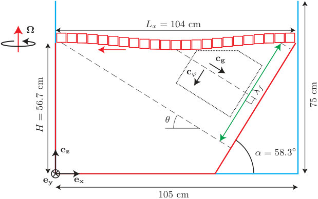 Figure 1
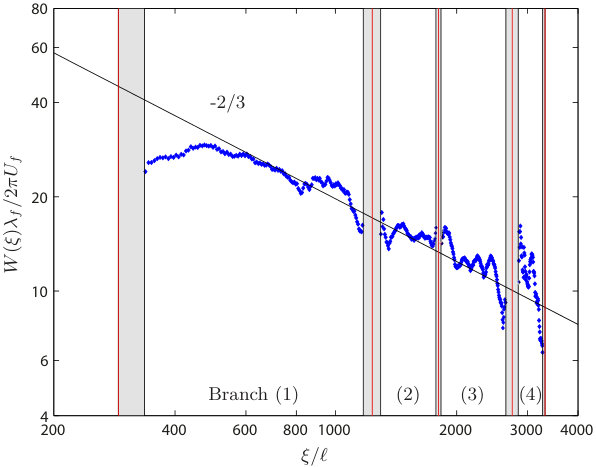 Figure 10
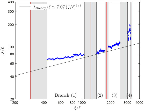 Figure 11
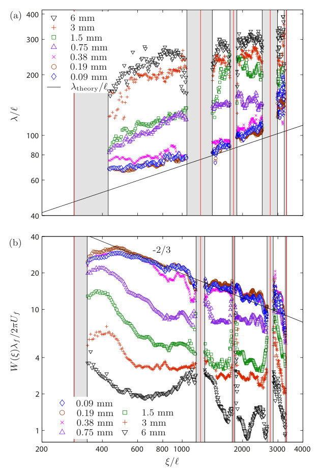 Figure 12
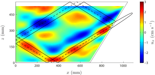 Figure 13
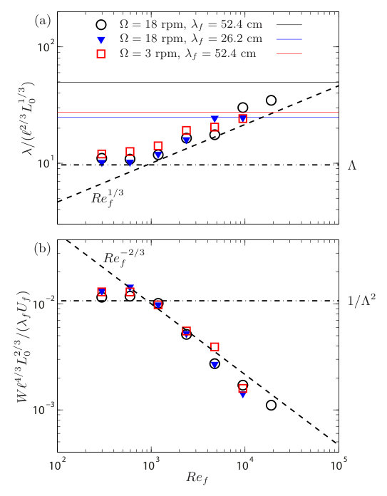 Figure 14
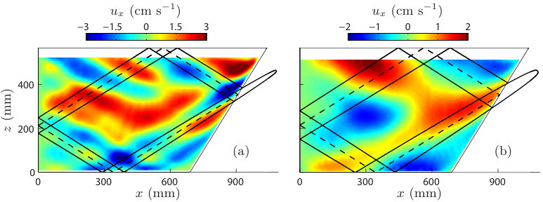 Figure 15
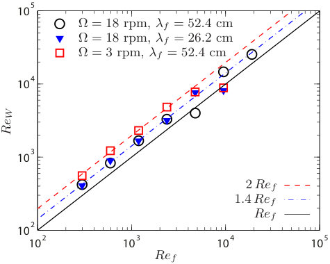 Figure 16
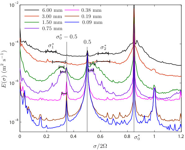 Figure 17
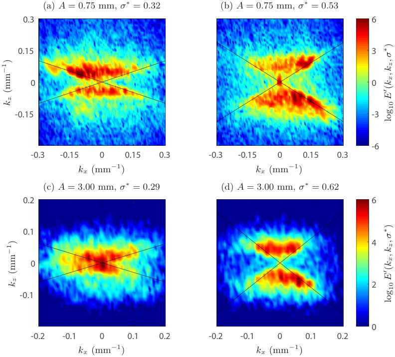 Figure 18
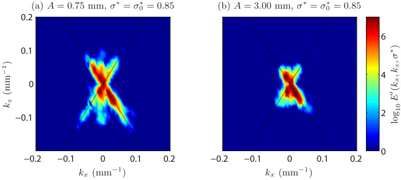 Figure 19
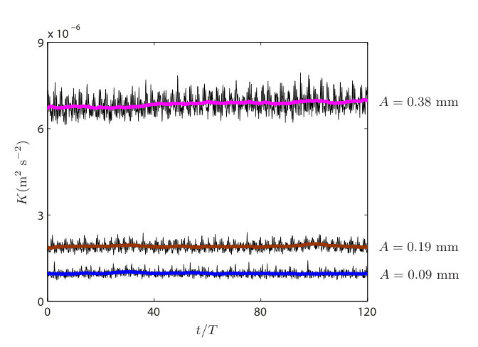 Figure 2
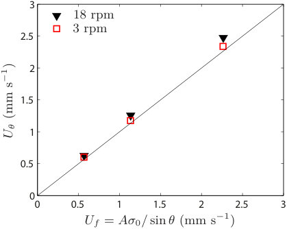 Figure 3
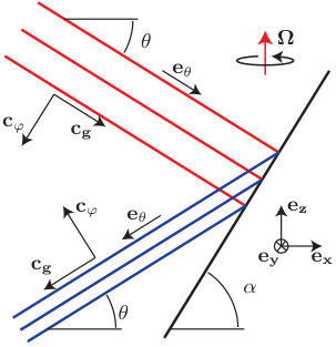 Figure 4
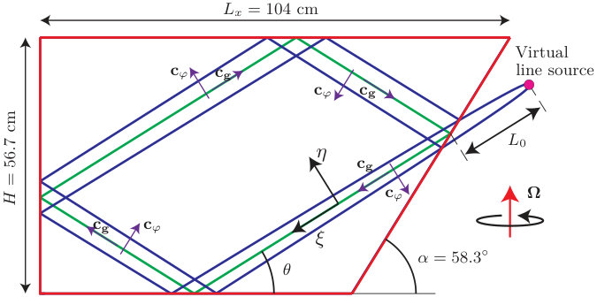 Figure 5
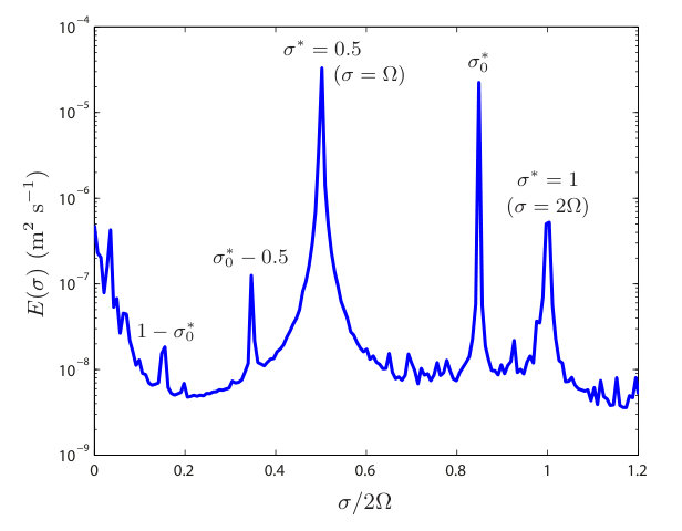 Figure 6
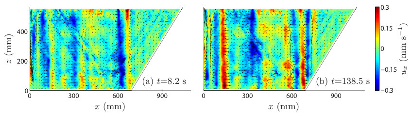 Figure 7
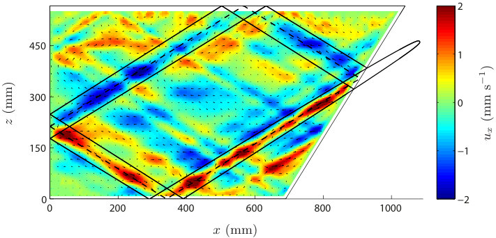 Figure 8
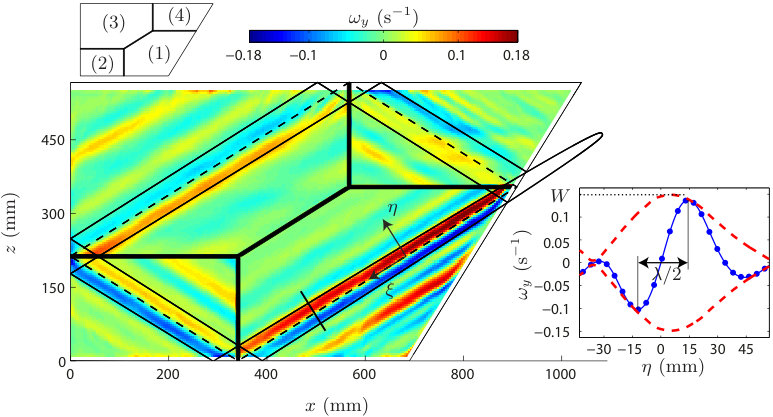 Figure 9
| (mm) | 0.09 | 0.19 | 0.38 | 0.75 | 1.50 | 3.00 | 6.00 |
|---|---|---|---|---|---|---|---|
| 300 | 600 | 1 190 | 2 380 | 4 750 | 9 500 | 19 000 | |
| — | — | 0.320.01 | 0.320.02 | 0.310.02 | 0.290.05 | 0.230.04 | |
| — | — | — | 0.530.02 | 0.540.02 | 0.620.05 | 0.640.04 | |
| — | — | — |
Peer Reviews
No public reviews on file for this paper yet. If you reviewed it on a platform where reviews are public (OpenReview, ICLR, NeurIPS, ICML), you can paste yours below so the community can read it here.
Videos
No videos yet. Explain this paper in a talk, walkthrough, or lecture? Add one.
Linear and nonlinear regimes of an inertial wave attractor
Maxime Brunet
Laboratoire FAST, CNRS, Université Paris-Sud, Université Paris-Saclay, 91405 Orsay, France
Thierry Dauxois
Université de Lyon, ENS de Lyon, Université Claude Bernard, CNRS, Laboratoire de Physique, F-69342 Lyon, France
Pierre-Philippe Cortet
Laboratoire FAST, CNRS, Université Paris-Sud, Université Paris-Saclay, 91405 Orsay, France
(March 8, 2024)
Abstract
We present an experimental analysis of the linear and non-linear regimes of an attractor of inertial waves in a trapezoidal cavity under rotation. Varying the rotation rate and the forcing amplitude and wavelength, we identify the scaling laws followed by the attractor amplitude and wavelength in both regimes. In particular, we show that the non-linear scaling laws can be well described by replacing the fluid viscosity in the linear model by a turbulent viscosity, a result that could help extrapolating attractor theory to geo/astrophysically relevant situations. We further study the triadic resonance instability of the attractor which is at the origin of the turbulent viscosity. We show that the typical frequencies of the subharmonic waves produced by the instability behaves very differently from previously reported numerical results and from the prediction of the theory of triadic resonance. This behavior might be related to the deviation from horizontal invariance of the attractor in our experiment in relation with the presence of vertical walls of the cavity, an effect that should be at play in all practical situations.
I Introduction
Fluids submitted to a global rotation enable the propagation of a specific class of waves, called inertial waves Greenspan1968 as a result of the restoring action of the Coriolis force. In an inertial wave, energy propagates in a direction tilted by an angle with respect to the horizontal which is defined by the dispersion relation
[TABLE]
where is the wave angular frequency and the fluid rotation rate around the vertical axis. Inertial waves are cousins of internal waves of gravity propagating in linearly stratified fluids Pedlosky1987 : they have similar dispersion relations linking the ratio between the wave frequency and the rotation rate or the buoyancy frequency to a specific direction along which their energy propagates. These dispersion relations lead to orthogonal group and phase velocities and also let the lengthscales of the wave unprescribed by the frequency. These lengthscales (wavelength, beam width) are consequently set by boundary conditions, viscous dissipation and eventually non-linearities. This leads to a variety of wave structures like self-similar wave beams Mowbray1967 ; Flynn2003 ; Cortet2010 ; Machicoane2015 , plane waves Mercier2010 ; Bordes2012 or resonant cavity modes Aldridge1969 ; McEwan1970 ; Maas2003b ; Boisson2012 ; Boisson2012b . These waves are relevant in geophysics and astrophysics in which they often merge into inertia-gravity waves with a single dispersion relation coupling rotation and buoyancy Lighthill1978 ; Pedlosky1987 . Considering pure inertial and pure gravity waves, a major difference however exists: gravity waves involve rectilinear fluid oscillations in the plane tilted by the angle whereas in inertial waves fluid particles describe anti-cyclonic circular translations in this plane.
In closed domains, modes of standing waves can be found for specific frequencies when the walls are normal and parallel to the rotation axis Greenspan1968 ; McEwan1970 but also in some geo/astrophysically relevant geometries such as spheres and spheroids Zhang2004 . In geo and astrophysics, several types of global forcing may be at the origin of such modes. For example, modes can be excited in spheres and spherical shells by a longitudinal libration Aldridge1969 ; Rieutord1991 ; Tilgner1999 ; Noir2009 ; Calkins2010 consisting in a time modulation of the rotation rate. Precession Busse1968 ; Kerswell1995 ; Noir2001 ; Boisson2012 and tidal deformation of the planet crust Suess1971 ; Morize2010 are other examples.
However, closed domains generally include sloping walls in which case the wave focusing and defocusing induced by the peculiar reflection laws of inertial/internal gravity waves Phillips1963 prevent the existence of cavity eigenmodes Maas1995 . It is a consequence of the dispersion relation: the wave keeps constant its propagation angle (in absolute value) with respect to the horizontal when reflecting on a wall. This implies for reflection on tilted walls that Snell-Descartes laws are not verified and that the wave lengthscales are enhanced or reduced depending on the fact the wave is descending or climbing the slope Phillips1963 . This peculiar physics can lead to the emergence of limit cycles, called wave attractors Maas1995 ; Maas1997 ; Rieutord2001 ; Manders2003 , on which the waves concentrate when excited in closed domains with tilted walls, including the astrophysically relevant case of spherical shells Rieutord2001 . From a theoretical point of view, tracing rays respecting the reflection laws directly reveals the existence (or the absence) of an attractor for a given wave frequency, via the convergence (or not) of all rays towards a unique limit cycle. Inviscid attractors actually exist over specific frequency ranges depending on the cavity geometry Maas1995 ; Maas1997 ; Rieutord2001 ; Manders2003 .
The first clear experimental observations of attractors were done in trapezoidal cavities by Maas and co-workers both for internal gravity waves Maas1997 and for inertial waves Maas2001 ; Manders2003 ; Manders2004 (and also latter in another geometry by Klein et al. Klein2014 for inertial waves). In these experiments, the wave forcing was realized through a global motion of the water tank: a longitudinal libration in the case of rotation and an oscillating vertical translation in the case of stratification. In reality, the energy injected at the forcing frequency does not focus on an infinitely thin parallelogram because of viscous dissipation. The scales (width and wavelength) of the attractor then follow from the competition of the energy focusing during reflections on tilted walls and the energy dissipation during wave propagation: focusing reduces scales whereas dissipation preferentially damps small scales. It has been proposed that the attractor wave beam once unwrapped can be described as a self-similar wave beam emitted by a virtual point source located upstream of the focusing reflection Rieutord2001 ; Ogilvie2005 ; Hazewinkel2008 ; Grisouard2008 . This model, in which the scale reduction at the focusing reflection is exactly compensated by the viscous spreading of the beam emitted by the point source Cortet2010 ; Machicoane2015 , has been tested with an increasing success in numerical simulations Grisouard2008 ; Jouve2014 .
Since in geo/astrophysics extremely large Reynolds numbers are involved, a particularly interesting, but not thoroughly discussed, facet of this problem is how the attractor is affected by non-linearities when increasing the forcing amplitude. This question has started to be explored experimentally by Scolan et al. Scolan2013 and Brouzet et al. Brouzet2017 in stratified fluids and by Jouve and Ogilvie Jouve2014 in direct numerical simulations of a rotating tilted square: they have revealed the emergence of an instability of the attractor feeding two subharmonic waves in triadic resonance with the attractor. This non-linear process has further been shown to affect the attractor by damping its amplitude and increasing its scales. These observations have been proposed to result from the additional effective dissipation that the instability induces for the attractor Jouve2014 ; Brouzet2017 . However, no scaling laws have up to now been identified to describe the non-linear evolution of the attractor. Even in the linear regime, it is not clear how the attractor amplitude scales with the forcing Reynolds and Rossby numbers.
In this article, we propose such scaling laws and compare them successfully with experimental data. We explore the linear and non-linear regimes of an inertial wave attractor in a trapezoidal cavity under rotation using a co-rotating particle image velocimetry system. The flow is generated by a deformable upper cover of the cavity which has a sinusoidal shape with a phase propagating horizontally. The dependencies of the scale and amplitude of the attractor are studied as a function of the forcing amplitude for several rotation rates and forcing wavelengths. This large data set allows us to validate scaling laws for the attractor in the non-linear regime which have been theoretically established assuming that the linear attractor model is still valid in the non-linear regime if one replaces the fluid viscosity by a turbulent viscosity. We further report a detailed study of the subharmonic waves produced by the triadic resonance instability responsible for the attractor non-linear evolution mentioned above. We show that, as the forcing Reynolds number is increased, the two typical frequencies, at which subharmonic waves are produced, are moving away from half the attractor frequency, in contradiction with what is expected from the theory of the triadic resonance instability as well as from numerical simulations of inertial wave attractors Jouve2014 . We suggest that these differences could be related to the three-dimensionality of fluid motions in inertial waves interacting here with the cavity vertical walls. We finally show that a significant amount of the waves produced by the instability are three-dimensional, breaking the invariance in one horizontal direction of the forcing and of the attractor, which could also be a consequence of the waves interaction with the vertical walls.
II Experimental setup
The flow is generated in a trapezoidal cavity of height cm, length cm and width cm as illustrated in Fig. 1. This cavity is contained in a parallelepipedic tank of cm2 base and cm height filled with cm of water. One wall of the cavity is a plate tilted by an angle with respect to the horizontal. The forcing of the flow is realized by the upper wall of the cavity which is made of a series of horizontal bars, cm long and centered in the tank in the direction. The bars have a square section of mm side in the plane and are spaced of mm in the direction. Each of these bars is connected to a linear motor able to drive it in a vertical motion. This wavemaker imposes the upper cover of the flow to approximate the following wavy shape
[TABLE]
where and two values of the wavelength have been considered: cm cm and cm cm ( cm is the size of an oscillating bar plus the interval between two bars). The whole system is mounted on a 2 m diameter platform rotating at a constant rate rpm or rpm about the vertical axis . The rotation of the platform is set at least 30 minutes before the wavemaker is started to avoid transient spin-up recirculations. The angular frequency of the wavemaker is set to . The amplitude of the bars motion is varied in the range [ mm, mm].
The two components of the velocity field are measured in the vertical plane using a particle image velocimetry (PIV) system mounted in the rotating frame ( is the front side of the tank). The fluid is seeded with 10 m tracer particles and illuminated by a laser sheet generated by a corotating 140 mJ Nd:YAG pulsed laser. Pairs of images of particles are acquired using two pixels cameras. Using a spatial calibration, the two images in each pair are combined into a single image covering the whole trapezoidal cavity. For wavemaker amplitudes mm, image acquisition consists of series of to image pairs recorded at a rate between and Hz depending on the wavemaker amplitude and on the rotation rate rpm or rpm. These values correspond to the acquisition of periods of the wavemaker with a time resolution between and image pairs per wavemaker period. For the wavemaker amplitudes larger than mm, acquisitions consist in the regular recording of two pairs of images separated by a time interval ms ms. This double-frame PIV configuration is rendered necessary by the large amplitude of the fluid velocity. For these large values of , to periods of the wavemaker are recorded with a time resolution of doublets of image pairs per wavemaker period. We finally compute cross-correlation between successive images over windows of pixels with overlap. This produces velocity fields of spatial resolution mm, with lines of between (at the bottom) and (at the top) vectors almost covering the whole section of the cavity. A few acquisitions have been realized during the transient settling of the flow after the wavemaker is started. They have revealed that a steady state is reached after a few dozen periods of the wavemaker forcing. In the data discussed in the following, image acquisition is started after 500 periods of the wavemaker oscillation. In order to illustrate the degree of statistical stationarity of the flow, we report in Fig. 2, the time series of the kinetic energy for three experiments, the angular brackets denoting the spatial average over the measurement plane.
In an unbounded domain, our wavemaker is expected to generate an inertial wave with its energy propagating at an angle with respect to the horizontal and of wavelength cm or cm (see Fig. 1). In line with Eq. (2), the phase of the wavemaker propagates toward decreasing values of , selecting the excitation of a wave with an energy propagating toward increasing (see the group and phase velocities in Fig. 1). A more subtle point is to predict the velocity amplitude of the raw wave excited by the wavemaker. Considering the small thickness of the Ekman boundary layers expected on the wavemaker, mm, one can assume that an effective free-slip condition holds at the scale of the wave Machicoane2018 . One can therefore expect that the wavemaker prescribes the -component of the velocity field. Since in an inertial wave fluid particles describe anticyclonic circular translation in planes tilted by the angle Greenspan1968 ; Bordes2012 ; Machicoane2018 , the amplitude of the wave velocity components (along directions and ) are expected to be mm s*-1*. This prediction is expected to hold when but probably fails when since it would imply a divergence of the wave velocity amplitude.
To confirm that this prediction holds at the angle used in the experiments, we have realized a few complementary experiments without the tilted plane. In Fig. 3, we report the velocity oscillations amplitude along the direction , i.e. the direction of the wave group velocity, as a function of the predicted amplitude . To get , we first Fourier filter the velocity field obtained from particle image velocimetry at frequency . We then compute the amplitude of the velocity oscillations along direction and finally take the spatial average of the resulting field over the region delineated by the dashed lines in Fig. 1 in the center of the excited wave. Figure 3 confirms that the excited wave amplitude is indeed close to within a precision which confirms the relevance of our estimate. The values found for are actually slightly larger than . This discrepancy can be the consequence of the fact that the assumptions made to model , i.e. the free-slip boundary condition and the fact that the wavemaker is watertight (which is not the case because of the 5 mm gap between the bars), are only valid to the first order. This discrepancy might also reveal the contribution to the measured velocity amplitude of the wave after its reflections on the four cavity walls which is superimposing to the original wave. In the following, and will be named forcing velocity and forcing wavelength and the forcing Reynolds number.
III Wave attractor in the linear regime and beyond
Attractors of internal waves of inertia or gravity can emerge in cavities with walls non-parallel or non-normal to the rotation or stratification axis. This is due to the anomalous reflection laws of these waves which keep constant their propagation angle with respect to the horizontal during a reflection Phillips1963 . As a consequence, when reflecting downwards on a wall tilted by an angle (see Fig. 4), a wave has its transverse lengthscales reduced by a factor
[TABLE]
Moreover, noting that the group velocity of a plane inertial wave of angular frequency has a magnitude , the conservation of the energy flux implies that and are conserved at reflection (at least in the inviscid case Beckebanze2018 ), being the wavelength and and the amplitude of the velocity oscillations along directions and respectively (see Fig. 4). Besides, the wave vorticity scaling as is amplified by a factor at the reflection.
In a closed domain, this focusing process leads, for certain geometry-dependent ranges of angles , to an energy concentration on a wave attractor Maas1995 ; Maas1997 ; Rieutord2001 ; Manders2003 . In the trapezoidal cavity considered here, a inertial wave attractor is expected when waves are generated with a propagation angle in the range between
[TABLE]
The notation corresponds to the simplest class of attractor in a trapezoidal cavity and follows from the nomenclature introduced in Maas1997 , the first number being the number of reflections on the bottom wall and the second the number of reflections on the sloping wall. The two limit angles and correspond to the slope of the diagonals of the trapezoidal cavity.
In Fig. 5, we show for the angle used in the experiments the unique closed parallelogram with its vertices on the walls of the cavity and its sides all tilted by an angle . This parallelogram corresponds to the inviscid wave attractor: ray tracing for any wave at will converge toward this parallelogram. The rate of convergence of the rays toward the inviscid attractor in a trapezoidal cavity has been characterized by Maas and co-workers in Maas1997 via the calculation of the Lyapunov exponents for each couple of non-dimensional geometric parameters (). In Maas1997 , internal gravity waves are considered, but since inertial waves behave exactly the same way regarding two-dimensional ray tracing, the Lyapunov exponents diagram as a function of () is expected to be identical in our case. This diagram reveals regions of strong convergence called Arnold tongue Maas1997 ; Brouzet2017b . In our experiments, one has () which falls in the middle of the Arnold tongue corresponding to the -attractor.
In a viscous fluid, the inviscid concentration of energy on a line attractor is prevented by viscous dissipation of waves during their propagation. The structure of the attractor can eventually be seen as the result of a balance between focusing at the sloping wall and the viscous spreading of a self-similar polychromatic wave beam Rieutord2001 ; Ogilvie2005 ; Hazewinkel2008 ; Grisouard2008 . As proposed in Grisouard2008 for internal wave attractors in a linearly stratified fluid, the four branches of the attractor, once unwrapped, can indeed be seen as part of a beam emitted by a virtual line source (invariant along the direction), located at a distance upstream of the focusing reflection (see Fig. 5).
From a general point of view, the wave beam excited by a line source has a self-similar transverse structure. Its velocity component along the propagation direction is given by (see Ref. Machicoane2015 for details)
[TABLE]
and the out-of-plane vorticity component by
[TABLE]
where is the distance from the source, the local transverse coordinate,
[TABLE]
a viscous scale and
[TABLE]
the scaling law followed by the width (and all other transverse length scales) of the beam. In the experiments, mm for rpm and mm for rpm. The functions and have been introduced by Moore and Saffman Moore1969 and Thomas and Stevenson Thomas1972 to describe self-similar wave beams of inertial and internal waves respectively. These real functions are defined by
[TABLE]
In Eqs. (6), (7) and (10), the integer corresponds to the multipolar order of the line source of waves as discussed in Machicoane2015 : corresponds to a monopolar source and to a dipolar source. Our wavemaker produces a large-scale wave with a zero instantaneous net mass flux (because of an integer number of wavelengths) which suggests to consider the dipolar case . However, it is worth noting that Jouve and Ogilvie Jouve2014 consider the case in their work which leads to a successful description of the spatial dependence of the attractor amplitude in their numerical simulations. The multipolar order of the virtual source to be considered here is therefore an open question.
Noting the length of the unwrapped inviscid attractor and the distance between the virtual source and the focusing point, the balance between the viscous spreading of the wave between and with lengthscales increasing as and the focusing reflection leads to the compatibility relation . In the experiments, the attractor length is cm such that cm (see Fig. 5). This eventually leads to the following relation for the transverse length scale of the attractor as a function of along-attractor coordinate Grisouard2008 ; Jouve2014 ; Brouzet2017
[TABLE]
Here, is the distance along the unwrapped attractor starting from the focusing reflection.
The relevance of the scaling law (11) has been first tested numerically for gravity waves in a stratified fluid by Grisouard and coworkers Grisouard2008 who indeed observed power law behaviors but with exponents departing from by and in the two reported configurations. In numerical simulations of a rotating tilted square, Jouve and Ogilvie Jouve2014 confirmed more clearly the predicted scaling laws for the attractor width and the velocity amplitude (case ) with the position along the attractor as well as the relevance of the Moore-and-Saffman transverse structure of the beam. From an experimental point of view, Brouzet et al. Brouzet2017 studied the evolution with time of the wavelength in the attractor during its transient growth and decay phases in a linearly stratified fluid. These data revealed a decrease toward a steady state value during the forced growth and a further decrease during the free decay. Comparable results were previously reported by Hazewinkel and coworkers Hazewinkel2008 .
Jouve and Ogilvie Jouve2014 also studied the non-linear regime of the attractor of inertial waves and showed the emergence of a local instability close to each focusing point. This instability transfers the energy of the wave attractor toward two subharmonic waves with their frequencies in triadic resonance with the primary wave frequency. This scenario is consistent with the one reported in internal gravity wave attractor experiments by Scolan et al. Scolan2013 . These local subharmonic instabilities of an internal wave attractor are actually very similar to instabilities of plane wave beams observed experimentally in rotating Bordes2012 and stratified Bourget2013 fluids. In this context, it has been shown Bourget2014 ; Karimi2014 that one should take into account the finite width of the wave beam, i.e. the small number of wavelengths contained in the transverse extension of the wave attractor (typically 1), in order to correctly predict the growth rate of the secondary waves generated by the instability.
In this context, one can highlight a remarkable feature of the instability of the experimental plane inertial wave reported by Bordes et al. Bordes2012 compared to all other mentioned instabilities: in the temporal spectrum, two wide bumps are observed, centered around two frequencies in triadic resonance with the primary wave frequency. This is in strong contrast with the internal gravity waves experiments with either a plane wave Bourget2013 or an attractor Scolan2013 but also with the inertial wave attractor simulations Jouve2014 for which the instability is very selective in terms of secondary wave frequencies. The physical origin of this specificity of experimental inertial waves remains unclear up to now.
Finally, in Jouve2014 and Brouzet2017 in which subharmonic triadic instabilities of numerical inertial and experimental internal wave attractors are reported, a thickening of the attractor beam is reported, as the forcing amplitude is increased. This thickening can be understood qualitatively as the consequence of the extraction of energy from the attractor at frequency by the triadic instability which acts as an effective turbulent dissipation: the instability then naturally produces an attractor with a smaller relative amplitude and larger transverse scales as the forcing amplitude is increased.
IV Experimental results
IV.1 Linear regime
In our experiments, energy is injected at frequency by the wave generator. In order to uncover the frequency content of the flow, we compute for each experiment the temporal power spectral density of the velocity field as
[TABLE]
where
[TABLE]
is the temporal Fourier transform of with , the angular brackets denote the spatial average over the measurement plane, is the acquisition duration and .
In Fig. 6, we report the temporal energy spectrum for the forcing wavelength cm and the lowest forcing amplitude mm at rpm as a function of the normalized frequency . This spectrum is mainly composed of a sharp peak at the forcing frequency as well as a secondary but energetic peak at the frequency of the rotating platform . The latter corresponds to a flow excited by the Earth rotation which induces a precession of the rotating platform (see Refs. Boisson2012 ; Triana2012 and references therein). In the case of a spherical or ellipsoidal cavity under precession, it is known as the tilt-over flow and has been extensively studied due to its relevance in astrophysics Kida2011 . One can also note the presence of energy at low frequencies . In a previous work of two authors of this paper using the same rotating platform Bordes2012 , it was shown that the energy peak at zero frequency (with a tail extending up to ) was already present when the flow forcing is off, suggesting that the low frequency spectral component is possibly the consequence of thermal convection in the water tank. The observation of the velocity field temporally smoothed over a large time-scale actually revealed the presence of columns which are slowly drifting in the water tank, resembling the columns observed in rotating thermal convection experiments Sakai1997 ; King2012 . Here, we observe the same kind of vertical columns, dominated by horizontal velocities, in the low-pass frequency filtered velocity field (two snapshots are shown in Fig. 7) which could possibly be the consequence of thermal convection. Nevertheless, even if no clear signs are observed here, one should let open the possibility that part of the energy present at very low frequencies in our experiments could be related to non-linearities —such as steady streaming Sauret2010 ; Bordes2012b or Stokes drift Sutherland2006 — affecting the flow motions at the forcing frequency or at the platform frequency . Other weakly energetic peaks are also present in the spectrum corresponding to the first harmonic of the tilt-over flow (), to interactions between the forcing and the tilt-over flow at and to interactions between the forcing and the first harmonic of the tilt-over flow at .
Overall, the flow produced by the wave generator with the lowest forcing amplitude at rpm seems to be in the linear regime. In order to discard the tilt-over and the low frequency flow components, we Fourier filter the velocity field at the forcing frequency . A snapshot of the corresponding field is reported in Fig. 8 to which is superimposed the width at mid-amplitude of the theoretical attractor (6). The velocity field reveals a concentration of energy along the theoretical attractor in good agreement with the theory. This concentration is however only partial since one can see other wave beams tilted by the angle outside of the region where the theoretical attractor is expected: in Fig. 8, the velocity magnitude in the attractor beam (from mm/s to mm/s) is actually only 3 to 7 times larger than the forcing velocity magnitude mm/s. As a consequence, since the wavemaker injects energy over the whole width of the water tank, we naturally find wave beams with a non-negligible amplitude outside of the attractor region.
To further compare the experimental flow at frequency and the theoretical attractor, we study its transverse profile as a function of the longitudinal coordinate along the inviscid attractor. To do so, we notice that each of the four branches of the attractor has its wavevector in a different quadrant of the wave vector plane (the wave vector is aligned with the phase velocity , see Fig. 5). We perform a Hilbert filtering of the velocity field (see Ref. Mercier2008 for details). It consists in computing the temporal Fourier transform of the raw velocity field, band-pass filtering the result around the frequency of interest (keeping only positive frequencies), and computing the inverse Fourier transform. We then take the two-dimensional (2D) spatial Fourier transform of the resulting complex field relative to and , put to zero the values of the resulting field except in the wavevector quadrant of interest, and finally compute the inverse 2D Fourier transform in space. Taking twice the real part of the result eventually provides the velocity field of the waves at frequency and with their wavevector in a given quadrant Mercier2008 . We finally perform a temporal phase average at phaseaverage . As an illustration, we report in Fig. 9 a snapshot of the field resulting from the Hilbert filtering: this snapshot is divided in four regions, each corresponding to a given theoretical attractor branch and to a Hilbert filtering selecting the wavevector quadrant of the theoretical attractor branch. One can note the presence of a few wave beams outside of the theoretical attractor which reveals that the focusing of the energy injected by the forcing in the attractor although clear is only partial.
In the inset of Fig. 9, we report a transverse profile (along ) of the out-of-plane vorticity component corresponding to the and Hilbert filtered velocity field. This transverse profile is taken at coordinate cm along the attractor axis (corresponding to the solid line in Fig. 9) at a given arbitrary phase, still for cm and the lowest forcing amplitude mm at rpm. We also report the corresponding experimental wave beam envelope where stands for the average on the phase . From such curves, we measure as a function of the longitudinal position , the beam vorticity amplitude as well as the wavelength estimated as the mean value over of twice the transverse distance between the maximum and minimum of the vorticity profile .
In Fig. 10, we report the vorticity amplitude for mm, cm and rpm as a function of coordinate along the unwrapped theoretical beam emitted by the virtual source. Data are missing on five portions of corresponding to the regions where the velocity field cannot be measured by PIV close to the reflections on the cavity walls. The attractor amplitude shows significant oscillations that are due to interferences of the wave attractor with the additional inertial waves at present in the cavity (see Fig. 8) as well as to interferences between two branches of the attractor close to a reflection. Nevertheless, one can observe a good agreement between the data and a power law of exponent in agreement with the scaling predicted by the theory (7) for a monopolar source of waves . The observation of this spatial decay exponent is consistent with the numerical data reported by Jouve and Ogilvie Jouve2014 . It shows that the multipolar order of the virtual point source to be considered in the attractor model is (monopolar source) and seems largely independent of the way energy is injected into the system.
In Fig. 11, we show the corresponding evolution with of the wavelength in the attractor, normalized by the viscous lengthscale (Eq. 8). As in Fig. 10, data are missing around the reflections on the cavity walls. The excluded ranges of are larger because estimates of the attractor transverse lengthscales are prevented when approaching a wall at distance of the order of these lengthscales (). We also report in Fig. 11 the theoretical prediction for according to Eqs. (7-10). We emphasize that this prediction is a power law in with a prefactor theoretically prescribed by the Moore-and-Saffman functions. One sees that, despite the fact that the power law behavior is not clearly observed in the data, the theory provides correct estimates for . The wavelength is found here always slightly larger than the theoretical prediction. Such a tendency is identical to the one reported for experimental gravity waves attractor Brouzet2017 . In this work as well as in Beckebanze2018 , it is proposed that the additional dissipation due to the viscous friction on the vertical walls of the cavity ( and ) leads to an attractor larger than in the 2D theory (invariant in the direction) by modifying the balance between energy focusing and viscous dissipation. One can finally highlight that in both Figs. 10 and 11, the experimental data in the fourth branch of the attractor are particularly noisy and also significantly departing from the theoretical scaling law. This could be understood by the fact that the fourth branch is the weaker in magnitude (see Eq. 6) whereas at the same time it is located where the original wave produced by the wavemaker is the strongest. The experimental data in the fourth branch of the attractor are therefore probably strongly affected by interferences between the wave in the attractor and the original wave produced by the wavemaker.
IV.2 Non-linear regime
We now repeat the previous analysis for increasing forcing amplitude . In Fig. 12, we report (a) the wavelength and (b) the out-of-plane vorticity amplitude normalized by the “forcing vorticity” as a function of the coordinate , for all forcing amplitudes at rpm and cm. One can see that the wavelength and the normalized vorticity amplitude are nearly identical for the three lowest forcing amplitudes indicating that the flow is in the linear regime. For larger values of the forcing amplitude , the transverse (cross-beam) wavelength of the beam increases whereas the normalized beam vorticity decreases with , indicating the emergence of non-linear effects. Figure 13, showing a snapshot of the velocity field Fourier filtered at for mm at rpm and cm, provides a direct illustration of the attractor thickening when increasing . In this figure, one still observes a concentration of energy around the theoretical attractor but this concentration is clearly less pronounced than for low (see Fig. 8).
In Fig. 14, we report, as a function of the forcing Reynolds number , (a) the wavelength and (b) the vorticity amplitude averaged over the first branch of the attractor (the one following the focusing reflection). Three data series are reported here for ( rpm, cm), ( rpm, cm) and ( rpm, cm). In Fig. 14(a), the wavelength is normalized by accounting for the dependence predicted by the linear attractor theory (9). We first note that the three data series collapse on a master curve. This suggests that the forcing Reynolds number is, to the first order, the parameter controlling the non-linear evolution of the attractor. The normalized attractor wavelength is close to the value predicted by the linear theory for and increases at larger as already observed in Fig. 12(a) ( is the average of the theoretical prediction over the attractor first branch; it is shown by the horizontal dashed-dotted line). One can however note that the normalized wavelength saturates at the larger Reynolds numbers for the series at ( rpm, cm) and ( rpm, cm). This saturation is easy to understand: the wavelength cannot be larger than the one of the forcing, since energy can only be transferred to smaller scales, via the focusing reflections. In Fig. 14(a), the horizontal solid lines (black, red and blue) show the normalized wavelength for the three series of experiments. This wavelength theoretically correspond to the wave excited by the wavemaker after one reflection on the sloping wall. It stands as an upper limit for the wavelength found in the first branch of the attractor. For the largest forcing amplitudes at ( rpm, cm) and ( rpm, cm), approaches this limit suggesting that almost no energy concentration in the attractor is observed. This is confirmed by the direct observation in Fig. 15 of two corresponding velocity fields at in which one typically sees the wave excited by the wavemaker reflecting on the sloping wall: the forcing wavelength being smaller than the theoretical wavelength expected for the non-linear attractor, energy cannot be supplied to the latter by the forcing. In comparison, for the data series at ( rpm, cm), the wavelength for the largest Reynolds number is still significantly lower than the excited wave original wavelength after one reflection , revealing a greater robustness of the energy concentration in an attractor to the increase of Reynolds number when the rotation or the injection scale are larger, i.e. when the forcing Rossby number is lower.
As mentioned in Sec. III, we expect that in an inviscid fluid the product of the velocity times the wavelength of an inertial wave is conserved during the reflection on a tilted wall. A tentative scaling law for the vorticity amplitude of the linear attractor is therefore where and are characteristic of the wave initially forced by the wavemaker and is the theoretical scaling for the linear attractor wavelength. In Fig. 14(b), we report the vorticity amplitude normalized by as a function of . This normalization collapses the three data series on a master curve which illustrates that catches the physics of the attractor amplitude in the linear and non-linear regime. We verify that this normalized vorticity is first constant at low forcing Reynolds number confirming the linear regime of the flow. A tentative estimate for the normalized attractor vorticity in the linear regime could be made by considering the theoretical value predicted by the linear model for the attractor wavelength, i.e. ( is the average over the first branch of the theoretical normalized attractor wavelength). This prediction for is reported with a horizontal dashed-dotted line in Fig. 14(b): one sees that it indeed provides a reasonable estimate of the attractor vorticity in the linear regime. This behavior is consistent with the fact that the wavelength matches the linear theory in Fig. 14(a) for the same Reynolds number range. At larger , the ratio decreases with revealing again the emergence of non-linearities.
Figure 14 altogether allows us to state that the attractor wavelength and vorticity amplitude follow the scaling laws predicted by the linear model but modified in the non-linear regime by prefactors function of the forcing Reynolds number
[TABLE]
When the wavelength predicted by (14) is larger than , no attractor can develop: a cutoff is therefore expected in (14-15) when . As we will see in the following, the thickening of the attractor and the decrease of its relative amplitude when increases above is correlated to the onset of a triadic resonance instability of the attractor. This instability drains energy from the mode at toward lower frequency modes. For the mode at , the instability can be seen as an additional dissipation to the viscous dissipation. A rudimentary but simple way to account for this additional dissipation is to replace the fluid viscosity by a turbulent viscosity . Doing so in the viscous length appearing in Eqs. (14-15) leads to and . Reporting the laws (14-15) with these expressions in Fig. 14(a-b) provides an excellent description of the attractor wavelength and amplitude, confirming the relevance of the concept of turbulent viscosity to understand the non-linear wave attractor. We note that no numerical prefactor have been used when reporting Eqs. (14-15) in Fig. 14.
In Fig. 16, we finally report the Reynolds number of the attractor defined as which is shown to increase linearly with the forcing Reynolds number , over the whole studied range. The ratio indeed seems to be nearly constant for a given rotation rate: it is remarkably almost unaffected by the onset of the attractor instability at . The ratio is nevertheless slowly dependent on with for rpm and for rpm. Since one would expect if a simple and single reflection of the forced wave is observed, the ratio can be seen as a quantifier of the presence of an attractor. Following (14-15), one has . The weak but clear dependence of with the rotation rate that we report here shows that and are weakly dependent on the cavity Ekman number in addition to the leading dependence on the Reynolds number . Since this weak dependence does not involve the forcing wavelength and amplitude , it might be related to the physics of Ekman viscous boundary layers on the walls of the cavity. We are however currently not able to propose an explanation for this behavior which is weak but significant.
IV.3 Triadic resonance instability
To further understand the non-linear evolution of the flow beyond the instability threshold of the attractor, we report in Fig. 17 the temporal energy spectrum (Eq. 12) for all experiments at rpm and cm. Beyond mm () at which the linear prediction for the attractor thickness and amplitude start to fail, we observe the emergence of two subharmonic bumps in the spectrum. The frequencies and around which the bumps are centered are consistent with a triadic resonance with the forcing frequency , i.e. , as can be seen in the Table 1. We recall that the energetic peak at frequency , i.e. , observed for the lower amplitudes corresponds to the “tilt-over” flow forced by the Earth rotation which induces a Coriolis force on the fluid moving in the laboratory Boisson2012 ; Triana2012 . This peak probably hides the expected second energy bump in the experiments at mm for which we report only one subharmonic frequency . We also highlight that the sharp peak observed at , i.e. , for the low forcing experiments corresponds to the interaction of this “tilt-over” flow with the forcing frequency .
In any case, we can highlight that the emergence of the subharmonic instability through a triadic resonance illustrated by Fig. 17 is fully correlated with the increase of the attractor lengthscale and to the damping of its normalized amplitude revealed in Figs. 12 and 14. The subharmonic bumps in the temporal spectra are wide, a feature that was already reported for the triadic resonance instability of an experimental plane inertial wave in Bordes2012 . It confirms that there is a specificity for experimental inertial waves with respect to internal waves Bourget2013 ; Scolan2013 and numerical inertial waves Jouve2014 for which triadic instability produces two precise frequencies.
In Fig. 17, for the two largest forcing amplitudes mm and mm ( and ), the subharmonic bumps become hardly distinguishable. We believe that this last feature does not mean that the instability has vanished since the total energy stored in the modes at subharmonic frequencies is still significant but spread over large frequency ranges. The horizontal error bars shown in Fig. 17 aim at representing qualitatively the uncertainty on the determination of the central frequency of the subharmonic bumps and . Thus, considering with precaution the spectra for the two largest amplitudes in Fig. 17, we can note that the separation between the bumps center frequencies and seem to increase with , and going further away from . The bumps seem at the same time to get wider whereas their amplitudes progressively decrease with relatively to the base level of the spectrum. These results are in discrepancy with the temporal spectra reported in Jouve2014 for numerical simulations of inertial wave attractor in which and are clearly defined by sharp peaks and tend toward as the forcing amplitude increases. These points remain to be understood and will be discussed in the section V.
To confirm that the flow components associated to the bumps at and are composed of inertial waves, we search in the following for the spatio-temporal signature of their dispersion relation. To do so, we compute for each experiment the normalized spatio-temporal power spectral density of the velocity field as
[TABLE]
where
[TABLE]
is the spatio-temporal Fourier transform of with and the angular brackets represent the average over wavenumber space (normalization by the energy at ).
In Fig. 18, we report this spatio-temporal spectrum for the experiments at rpm, cm and mm () or mm (), for the respective center frequencies of the bumps in their temporal spectrum. Black lines represent the dispersion relation of 2D inertial waves invariant in the direction i.e. with . In such a representation, inertial waves with their wavevector in the measurement plane will appear through energy concentration on the black lines.
In Fig. 18, the energetic regions of the spatio-temporal spectra ressemble a sandglass with several maxima of energy along the black lines. This shows that the flow component at frequencies and is composed of inertial waves of which a significant proportion has a non-zero wavevector component along direction. Indeed, the general expression of the dispersion relation is , and inertial waves with will show up with energy in the regions between the two black lines () and containing the axis . Considering other forcing amplitude and other frequencies inside the subharmonic bumps of the temporal spectra leads to similar spatio-temporal spectra. The only exception is the spatio-temporal spectra at the forcing frequency in which the energy is clearly concentrated on the black lines as can be seen in Fig. 19 (same experiments as in Fig. 18). This result confirms that the attractor remains nearly two-dimensional, with , in the measurement plane . For other frequencies , the presence of waves with wavevector in the measurement plane is natural since the triadic instability of an attractor invariant in the direction leads to such waves if no spontaneous breaking of symmetry appears. Waves found here with might be the fruit of the non-perfect -invariance of the experimental attractor due to the finite size in the direction of the wavemaker and/or to the presence of viscous boundary layers on the vertical walls of the cavity at and which both should lead to some three-dimensionality of the flow. This three-dimensionality might also be at the origin of the previously highlighted differences (bumps spreading in frequency and moving away from each other with increasing ) of the temporal spectra with the simulations of Jouve and Ogilvie Jouve2014 which were strictly 2D, invariant along direction.
V Conclusion
In this article, we have reported PIV measurements of the flow generated by a large-scale harmonic inertial forcing in a trapezoidal cavity with a tilted wall submitted to a global rotation. In the linear regime, we observe a concentration of the energy along a limit cycle inside the cavity as expected from the theory of internal wave attractors. Our data shows that the model, initially proposed by Rieutord et al. Rieutord2001 followed by Grisouard et al. Grisouard2008 and Jouve and Ogilvie Jouve2014 , describing attractors as a portion of a self-similar wave beam emitted by a virtual point source upstream of the tilted wall accounts correctly for the measured values of the wavelength in the attractor as well as for the scaling laws of the spatial decay of its amplitude.
We have further explored the non-linear regime of the attractor. The observed scenario is the following when increasing the forcing amplitude. The attractor becomes unstable beyond a forcing Reynolds number of . This instability feeds inertial waves gathered around two subharmonic frequencies and resonant with the attractor frequency . This triadic resonance instability is accompanied by a thickening in size and a damping in relative amplitude of the attractor as the forcing amplitude grows above the instability threshold. In parallel, the two bumps corresponding to the subharmonic waves in the temporal spectrum have their central frequencies and gradually moving away from while the bumps spread over wider ranges of frequencies tending to build a continuum of energy in frequency.
In Brouzet2017 , from similar experiments with internal gravity waves, Brouzet et al. also report an increase of the attractor wavelength and a reduction of its relative amplitude when the attractor becomes unstable via a triadic resonance. They interpreted their results by introducing a turbulent viscosity accounting for the fact the instability creates a sink of energy for the attractor. In this article, by considering data for two different rotation rates and for two forcing wavelengths , we have demonstrated that the attractor mean wavelength and vorticity amplitude follow scaling laws predicted by the linear attractor model even in the non-linear regime if one uses the turbulent viscosity based on the forcing velocity and wavelength in place of the fluid kinetic viscosity. This framework eventually predicts that the attractor wavelength and vorticity follow power laws and with the forcing Reynolds number beyond the onset of the triadic instability which scalings are in clear agreement with our data.
Regarding the subharmonic waves produced by the instability, it is worth highlighting two major differences with previous results Jouve2014 ; Scolan2013 ; Bourget2013 ; Brouzet2017 . The first one relies on the fact that the instability provides energy to large ranges of frequencies and not to two precise subharmonic frequencies. This weak selectivity is not specific to attractors since it has also been reported for a plane inertial wave beam Bordes2012 . It is in clear discrepancy with the strong selectivity reported for numerical inertial waves Jouve2014 . It might be related to the three-dimensional nature of the velocity oscillations in inertial waves: in a -invariant () wave at frequency , fluid particles describe circular translations in planes tilted by an angle and velocity oscillations are observed in the three directions , and . The vertical walls of the cavity are therefore incompatible with such -invariance in inertial wave experiments. This feature is on the contrary absent in 2D numerical simulations of inertial waves in which periodic boundary conditions are used in the direction Jouve2014 . In the case of internal gravity waves Scolan2013 ; Bourget2013 ; Brouzet2017 , for which fluids particles oscillate only in the vertical plane (), the physical vertical walls and are compatible with inviscid boundary conditions. The three-components character of inertial waves interacting with physical walls therefore appears as a good candidate to explain the weak selectivity of the triadic instability. This could be tested by comparing the results of numerical simulations with periodic boundary conditions and with walls at and . In this context, it is worth noting that Manders and Maas Manders2004 have studied the three-dimensional structure of an experimental inertial wave attractor forced by a libration perturbation of the global rotation in a trapezoidal cavity. The dependence of the experimental attractor in the -direction is however probably strongly different compared to the one in the data we report here since the libration forcing is anti-symmetric for mirror reflection with respect to the plane , leading to a phase shift of in the attractor between half-space and half-space . The libration forcing actually induces an oscillating horizontal circulation in the plane with strong horizontal velocities close to the vertical walls which is also a feature absent in our experiments.
A last major difference with previous works is that the instability of the inertial wave attractor reported here leads to subharmonic waves with frequencies more and more remote from as the forcing amplitude grows. This behavior is the opposite of the one reported in numerical simulations of an inertial wave attractor in a tilted square Jouve2014 . It is also in apparent contradiction with the theory of triadic instability of plane inertial/internal waves Koudella2006 ; Bordes2012 which predicts that the frequencies of the two subharmonic waves tend toward as the Reynolds number of the primary wave increases. This behavior is probably the most intriguing that has been reported here.
Acknowledgements.
We acknowledge M. Rabaud and F. Moisy for fruitful discussions, and J. Amarni, A. Aubertin, L. Auffray and R. Pidoux for experimental help. This work has been supported by the Agence Nationale de la Recherche through Grant “DisET” No. ANR-17-CE30-0003.
The reference list from the paper itself. Each links out to its DOI / PubMed record.
- 1(1) H. Greenspan, The Theory of Rotating Fluids (Cambridge University Press, Cambridge, UK, 1968).
- 2(2) J. Pedlosky, Geophysical Fluid Dynamics (Springer-Verlag, New York, 1987).
- 3(3) D.E. Mowbray and B.S.H. Rarity, A theoretical and experimental investigation of the phase configuration of internal waves of small amplitude in a density stratified liquid, J. Fluid Mech. 28 , 1 (1967).
- 4(4) M. R. Flynn, K. Onu, and B. R. Sutherland, Internal wave excitation by a vertically oscillating sphere, J. Fluid Mech. 494 , 65 (2003).
- 5(5) P.-P. Cortet, C. Lamriben, and F. Moisy, Viscous spreading of an inertial wave beam in a rotating fluid, Phys. Fluids 22 , 086603 (2010).
- 6(6) N. Machicoane, P.-P. Cortet, B. Voisin, and F. Moisy, Influence of the multipole order of the source on the decay of an inertial wave beam in a rotating fluid, Phys. Fluids 27 , 066602 (2015).
- 7(7) M. Mercier, D. Martinand, M. Mathur, L. Gostiaux, T. Peacock, and T. Dauxois, New wave generation, J. Fluid Mech. 657 , 310 (2010).
- 8(8) G. Bordes, F. Moisy, T. Dauxois, and P.-P. Cortet, Experimental evidence of a triadic resonance of plane inertial waves in a rotating fluid, Phys. Fluids 24 , 014105 (2012).