The Spectrum of Delay Differential Equations with Multiple Hierarchical Large Delays
Stefan Ruschel, Serhiy Yanchuk

TL;DR
This paper analyzes the spectral properties of delay differential equations with multiple large delays, revealing a hierarchical structure in their spectra that determines stability and destabilization mechanisms.
Contribution
It introduces a detailed spectral analysis framework for equations with multiple hierarchical delays, identifying strong and pseudo-continuous spectra and their roles in stability.
Findings
Spectrum splits into strong and pseudo-continuous parts
Strong spectrum converges to eigenvalues of $A_0$ as delays grow
Pseudo-continuous spectrum exhibits hierarchical structure and influences stability
Abstract
We prove that the spectrum of the linear delay differential equation with multiple hierarchical large delays splits into two distinct parts: the strong spectrum and the pseudo-continuous spectrum. As the delays tend to infinity, the strong spectrum converges to specific eigenvalues of , the so-called asymptotic strong spectrum. Eigenvalues in the pseudo-continuous spectrum however, converge to the imaginary axis. We show that after rescaling, the pseudo-continuous spectrum exhibits a hierarchical structure corresponding to the time-scales Each level of this hierarchy is approximated by spectral manifolds that can be easily computed. The set of spectral manifolds comprises the so-called asymptotic continuous spectrum. It is shown that…
Click any figure to enlarge with its caption.
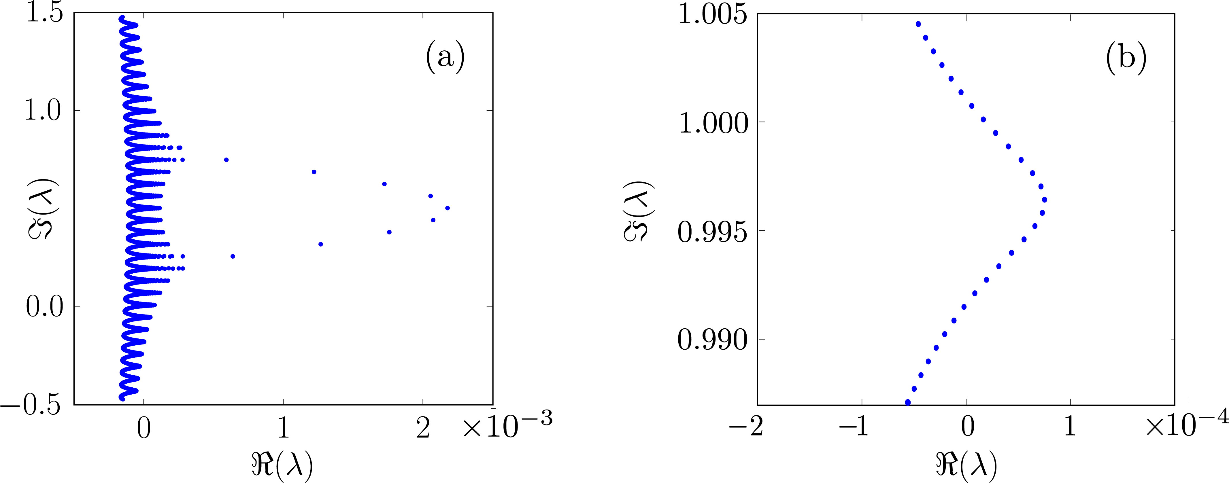 Figure 1
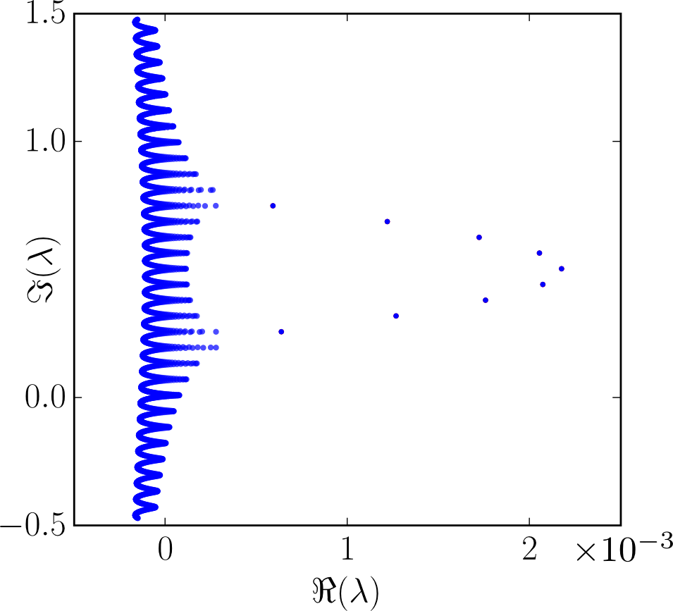 Figure 1
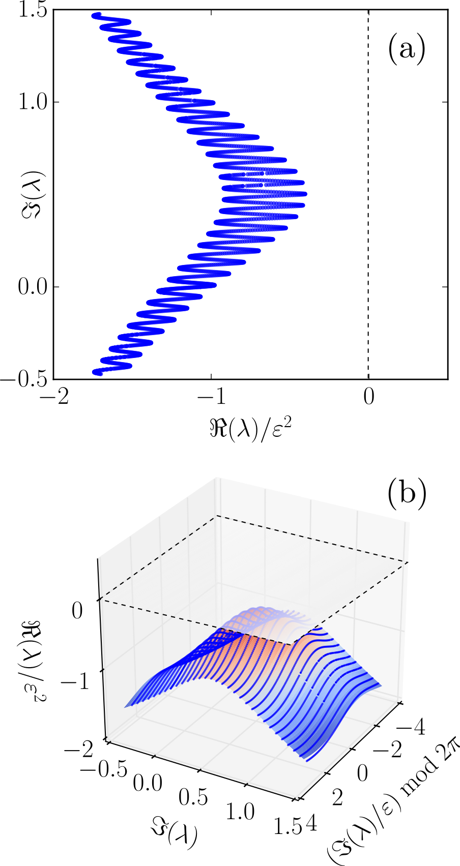 Figure 2
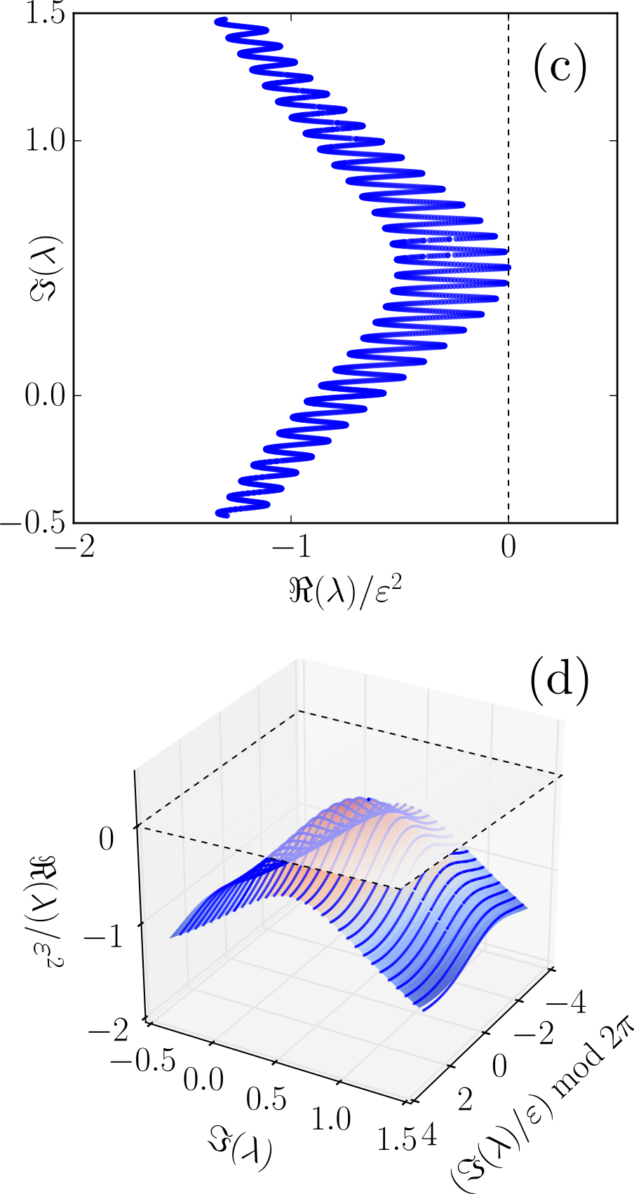 Figure 2
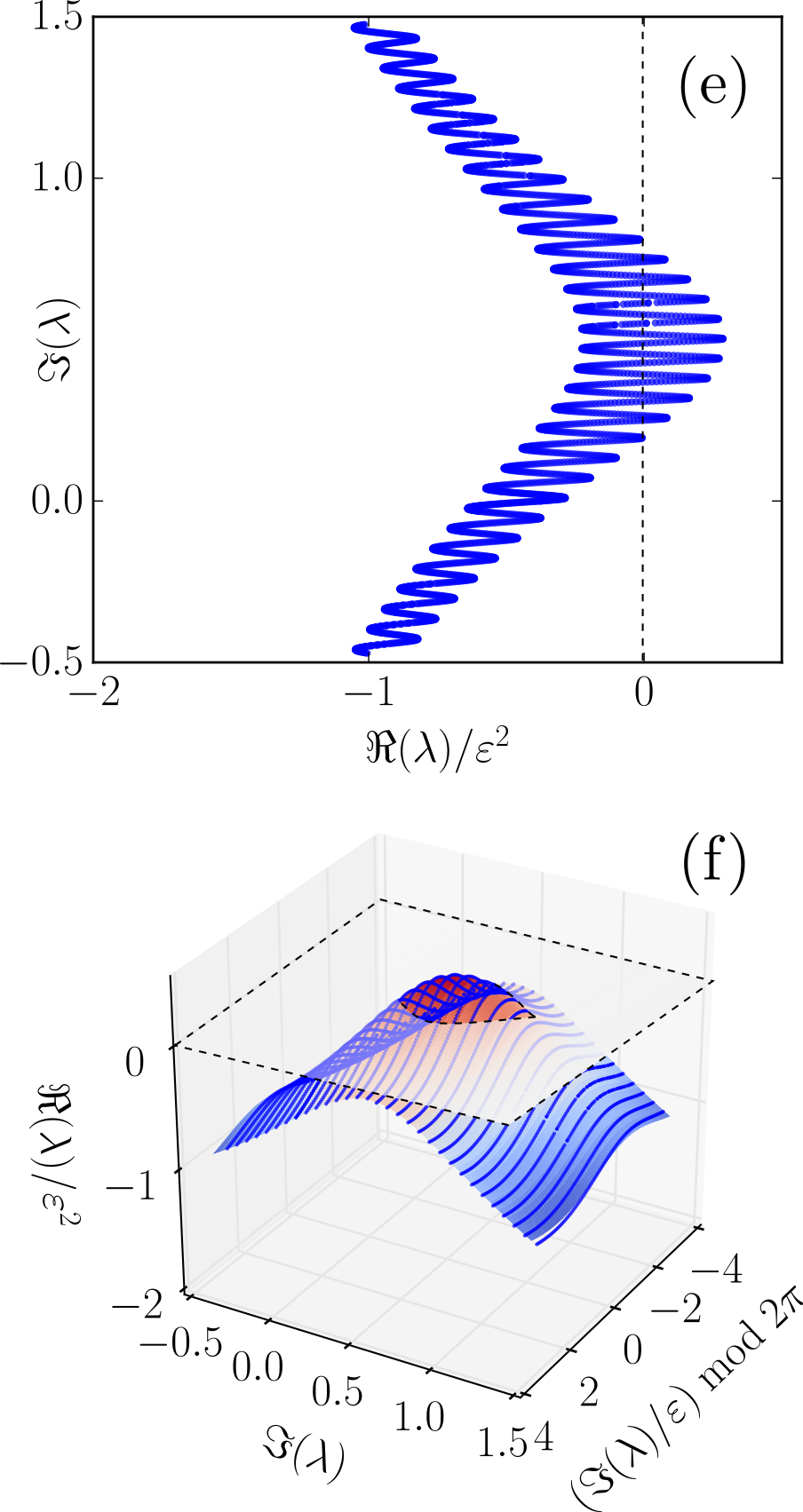 Figure 2
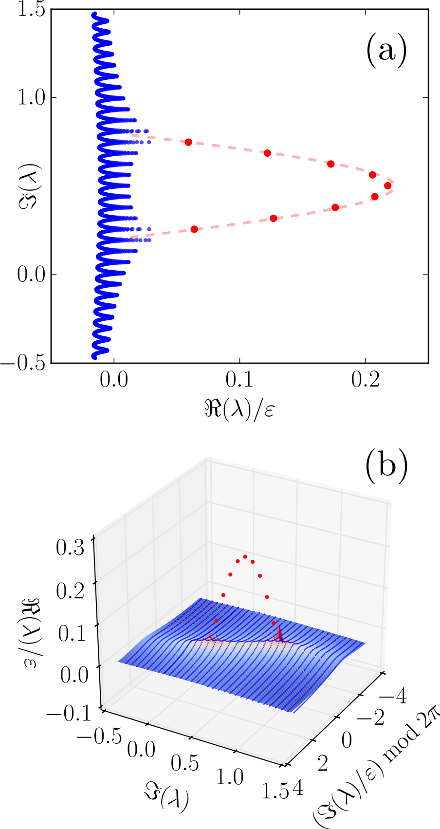 Figure 3
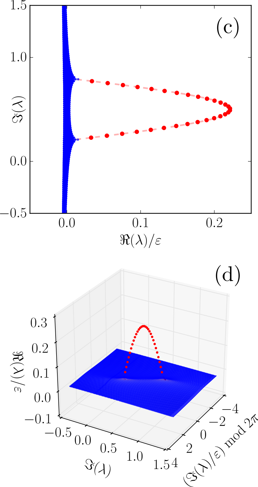 Figure 3
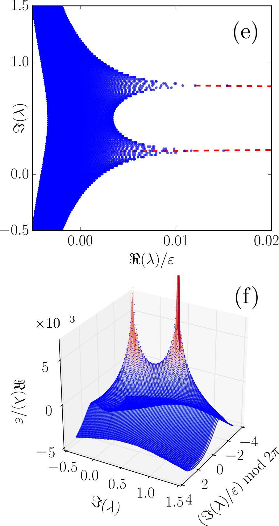 Figure 3
| Symbol | Description | Reference |
| Spectrum | Eq. (5) | |
| Strong spectrum | Def. 2.3, Eq. (15) | |
| Pseudo-continuous spectrum | Def. 2.3, Eq. (16) | |
| Truncated stable -spectrum | Def. 2.1, Eq. (10) | |
| Asymptotic strong spectrum | Def. 2.3, Eq. (14) | |
| Asymptotic strong unstable spectrum | Def. 2.3, Eq. (13) | |
| Asymptotic strong stable spectrum | Def. 2.1, Eq. (11) | |
| Asymptotic continuous -spectrum | Def. 2.4, Eq. (21) | |
| Asymptotic continuous stable -spectrum | Def. 2.4, Eq. (19) | |
| Asymptotic continuous unstable -spectrum | Def. 2.4, Eq. (20) | |
| Coefficient matrix corresponding to delay | Eq. (1) | |
| Projection of coefficient matrix to the | ||
| cokernels of matrices , | Eq. (9) | |
| Characteristic function | Eq. (6) | |
| Projected characteristic equation, | Def. 2.1, Eq. (8) | |
| Truncated characteristic equation, | Def. 2.4, Eqs. (17)–(18) |
| relevant asymptotic spectra | parameters | ||
|---|---|---|---|
| present (unstable) | |||
| not present | |||
| present (unstable) | |||
| not present | |||
| singular points | |||
| unstable | |||
| stable | |||
| singular points | |||
Peer Reviews
No public reviews on file for this paper yet. If you reviewed it on a platform where reviews are public (OpenReview, ICLR, NeurIPS, ICML), you can paste yours below so the community can read it here.
Videos
No videos yet. Explain this paper in a talk, walkthrough, or lecture? Add one.
The Spectrum of Delay Differential Equations with Multiple Hierarchical Large Delays
Stefan Ruschel
Department of Mathematics, University of Auckland, Auckland 1142, New Zealand
and
Serhiy Yanchuk
Institut für Mathematik, Technische Universität Berlin, Strasse des 17. Juni 136, 10623 Berlin, Germany
Abstract.
We prove that the spectrum of the linear delay differential equation with multiple hierarchical large delays splits into two distinct parts: the strong spectrum and the pseudo-continuous spectrum. As the delays tend to infinity, the strong spectrum converges to specific eigenvalues of , the so-called asymptotic strong spectrum. Eigenvalues in the pseudo-continuous spectrum however, converge to the imaginary axis. We show that after rescaling, the pseudo-continuous spectrum exhibits a hierarchical structure corresponding to the time-scales Each level of this hierarchy is approximated by spectral manifolds that can be easily computed. The set of spectral manifolds comprises the so-called asymptotic continuous spectrum. It is shown that the position of the asymptotic strong spectrum and asymptotic continuous spectrum with respect to the imaginary axis completely determines stability. In particular, a generic destabilization is mediated by the crossing of an -dimensional spectral manifold corresponding to the timescale .
Key words and phrases:
Linear Delay Differential Equations, Large Delay, Multiple Delays.
The authors acknowledge support by the Deutsche Forschungsgemeinschaft (DFG, German
Research Foundation) - Project 411803875 and SFB 910. The research was conducted while SR was doctoral student at Technische Universität Berlin.
1. Introduction
Delay Differential Equations (DDE) are highly relevant in various fields of applications including secure communication [1], information processing [2], and many others [3, 4, 5]. When studying these - generally nonlinear - equations close to equilibrium, one is first concerned with the spectral properties of a corresponding linearized system of the form [6, 7, 8, 9]
[TABLE]
A complete description of the spectrum of (1) can be formidable task even for a single delay, and is generally unfeasible for two or more. Specific cases therefore have been studied in much detail, see [10, 11, 12, 13, 14] and references therein. It is convenient however, if the involved time delays are large. In this paper, we provide a detailed description of the spectrum of (1) with finitely many large hierarchical delays
[TABLE]
which bear some analogy to spatially extended systems [15, 16]. Figure 1 provides an example of such a spectrum. One can observe a complicated structure and that there is a large number of eigenvalues that are very close to the imaginary axis, i.e. they play important role for determining stability. This manuscript provides not only an analytical description of such spectra, but also explicit analytic expressions for their approximations.
Examples for DDEs with multiple large hierarchical delays can be drawn from non-linear optics, where the finite-time communication delays are typically much larger than the device’s internal timescales [17]. Specific examples of (1) for two hierarchical large delays of different size include semiconductor lasers with two optical feedback loops of different length [18, 19, 20, 21], and ring-cavity lasers with optical feedback [22, 23, 24]. Additional examples can be found in applications to biological systems, when a corresponding separation of time-scales is justified [25, 26, 27, 28].
This work extends the results of [29] to multiple large hierarchical delays, under more general non-genericity conditions. We show that the spectrum splits into two distinct parts with different scaling behavior: the strong spectrum and the pseudo-continuous spectrum. As the delays tend to infinity, the strong spectrum converges to specific eigenvalues of , the so-called asymptotic strong spectrum. Eigenvalues in the pseudo-continuous spectrum converge to the imaginary axis as the delays increase. We show that after rescaling the pseudo-continuous spectrum exhibits a hierarchical structure corresponding to the time-scales In particular, we show that this set of eigenvalues can be represented as a union of subsets corresponding to different timescales . Generically, for , each of these sets can be associated with a -dimensional spectral manifold in the positive half plane that extends to the negative half-plane under certain degeneracy conditions related to the rank of the matrices or if . These manifolds can be computed explicitly and the corresponding eigenvalues can be found by projecting the manifolds to the complex plane. Moreover, the asymptotic spectra are exact at the imaginary axis, and therefore, the stability boundaries are completely determined by the position of the asymptotic strong spectrum and asymptotic continuous spectrum with respect to the imaginary axis. It is shown that a generic destabilization of such a system takes place by the crossing of an -dimensional spectral manifold corresponding to the timescale . Section 2 contains an overview of our rigorous results, along with an introduction to the needed basic concepts. The corresponding proofs contained in Sec. 4 are largely influenced by the proofs in [29]. Similar, to the single large delay case [30], our results in part can be extended to linear DDEs with time varying coefficients, see Ref. [31] for more details.
Aiming at a rigorous description, the presentation in Sec. 2 sometimes appears technical. We included Table 1 for quick referencing of frequently used notation throughout the article. To illustrate our results and to foster understanding of the main ideas, we present an example of analytically and numerically computed spectra for the scalar case with two large hierarchical delays in Sec. 3.
2. Basic concepts and Overview of Results
We consider the special case of hierarchical time delays , where , , and is a small parameter. Hence, we consider the linear Delay Differential Equation (DDE)
[TABLE]
with hierarchical large delays and study the asymptotic behavior of its solutions as . Throughout, we assume that is a complex-valued, Euclidean vector of size and are given matrices independent of time and . Existence and uniqueness of solutions to (3), as well as the specific notions of solution and state space will not be covered here, but can be found in classic text books on Delay and Functional Differential Equations [7, 8, 6].
Equation (3) can be thought of as similar in spirit to an Ordinary Differential Equation (ODE) except that it may exhibit so-called small solutions; those are solutions that “collide” with the trivial solution in finite time, say , and equal zero for all . Apart from this peculiarity, that is up to small solutions, any solution of (3) can be written as a superposition of exponential functions as in the case of ODEs [7]. In particular, the long term behavior of the solution as is governed by the characteristic exponents.
In this sense, solving (3) is equivalent to finding nontrivial solutions to the matrix-valued quasi-polynomial equation where
[TABLE]
is the characteristic matrix. A nontrivial solution exists, if and only if there is such that , or equivalently . For simplicity, let us assume is a simple root of . Together with a corresponding , it gives rise to a solution of Eq. (3). See Ref. [7] for further details. The pair is called an eigenvalue-eigenvector pair and the entirety of eigenvalues is called the spectrum
[TABLE]
of (3).
Hence, the problem consists of describing the asymptotic location of complex-valued solutions to the characteristic equation
[TABLE]
as . For each fixed , much is known about the solutions of (6). Firstly, there are countably many solutions that continuously depend on parameters. Secondly, the real parts of solutions accumulate at . Within each vertical stripe there are only finitely many solutions [6, 7]. In particular, can be chosen [7]. The following Secs. 2.1–2.3 present our main results. At first, it is convenient to discuss the non-generic case when some of the matrices do not have full rank, starting from highest order . In this case, one can immediately identify spectral subsets of truncated characteristic equations that approximate certain subsets of for sufficiently small .
2.1. Degeneracy spectrum
From the point of view of applications, we certainly cannot expect the matrices to be invertible. In this section, we introduce the necessary conditions for our main Theorem 2.5 to hold. To set the stage, consider the case when is not invertible. Then, for sufficiently small we may think of Eq. (6), as a low rank perturbation of a certain truncated characteristic equation, see Theorem 2.2. Let us explain. If , there exist unitary matrices such that
[TABLE]
where is a diagonal matrix of full rank, and is the conjugate transpose of . Equation (7) is the singular value decomposition of and the columns of and are the left and right singular vectors of , respectively.
The columns of the matrices and are the left and right singular vectors corresponding to the cokernel ( and ) and image ( and ) of . In particular, and , correspond to the projection onto the cokernel and image of , respectively. This projection allows to define the following spectral sets.
Definition 2.1** (non-generic spectral subsets).**
Let .
- (i)
Define as the matrices containing the left and right singular vectors of corresponding to the singular value zero. Denote
[TABLE]
[TABLE]
and the corresponding projected characteristic equation
[TABLE]
The set
[TABLE]
is called the truncated stable -spectrum. 2. (ii)
If is again not invertible, this procedure is applied iteratively. Recursively for all (starting from ), if , define (notice the tilde notation) containing left and right singular vectors of corresponding to the singular value zero. Denote
[TABLE]
[TABLE]
and the corresponding truncated characteristic equation
[TABLE]
for , and
[TABLE] 3. (iii)
Define as the smallest index such for all and . 4. (iv)
For define set
[TABLE]
for , and otherwise. The set is called the truncated stable -spectrum. If set
[TABLE]
and otherwise. is called asymptotic strong stable spectrum. 5. (v)
If and , define the matrices containing left and right singular vectors of corresponding to the singular value zero.
These sets correspond to spectral directions along which Eq. (1) acts as a DDE with fewer delays or even an ODE. Before stating our result, we have to guarantee that Eq. (1) is indeed a DDE and cannot be transformed into a system of ODEs through variable transformations, one has to demand the following non-degeneracy condition.
Condition (ND). If \det$$A_{n}=0, and then .
This is a rather abstract condition. In order to build some intuition, consider the following example. Let , and the matrices and are given by
[TABLE]
Clearly, and one readily computes
[TABLE]
as well as
[TABLE]
We may set . Condition (ND) then reads
[TABLE]
If , the system is degenerate; it corresponds to an ODE. Straightforward computation shows that the (general) characteristic equation
[TABLE]
does not depend on in this case, and the spectrum consists of for all . On the basis of Def. 2.1, the following Theorem 2.2 provides a hierarchical approximation of
[TABLE]
by spectral subsets of truncated characteristic equations , when some of the matrices do not have full rank.
Theorem 2.2**.**
Let \det$$A_{n}=0, be such that , and (ND) be satisfied. Further, let be sufficiently small and ( for k=0). Then there exits a small neighborhood of such that the number of eigenvalues equals the multiplicity of as a zero of .
The following Sec. 2.2 shows that eigenvalues with positive real part can be approximated in a similar way.
2.2. Hierarchical splitting and asymptotic spectrum
Consider the case when there exists an eigenvalue with a positive real part for an arbitrary small . It is easy to see that
[TABLE]
where is an induced matrix norm. If the real part of is uniformly bounded from zero, we have as . Therefore, the limiting solution is an eigenvalue of with positive real part (if it exists). This suggests that part of the spectrum (the so-called strong unstable spectrum, see Definition 2.3) with this specific scaling property can be approximated by eigenvalues of with positive real part, and we expect an error which is exponentially small in as (Theorem 2.5).
Definition 2.3**.**
Let
[TABLE]
The set
[TABLE]
is called the asymptotic strong unstable spectrum and the set
[TABLE]
is called the asymptotic strong spectrum. Let denote the set of balls around a set Let and
[TABLE]
then the sets
[TABLE]
are called strong unstable spectrum, strong stable spectrum and strong spectrum, respectively. The set
[TABLE]
is called the pseudo-continuous spectrum.
can be obtained by formal truncation of the characteristic equation after , i.e. neglecting the terms including delays. Note that Sec. 2.1 provides conditions under which is possible that also specific eigenvalues with negative real part can be approximated by eigenvalues of (see Theorem 2.5.(ii)). Analogously, one defines the following truncated expressions of higher order: Similar to our observation above, we have a splitting of the spectral subsets with respect to the different time scales corresponding to the hierarchy of delays. Consider an eigenvalue with real part asymptotically as and . Then has the leading order representation
[TABLE]
as . This observation motivates the following definitions.
Definition 2.4**.**
Define the functions , ,
[TABLE]
and the corresponding asymptotic spectra
[TABLE]
The sets
[TABLE]
are called the asymptotic continuous unstable -spectrum for all respectively. is called the asymptotic continuous -spectrum.
If , additionally define ,
[TABLE]
and if , ,
[TABLE]
and the corresponding asymptotic continuous spectra
[TABLE]
The sets
[TABLE]
are called the asymptotic continuous stable -spectrum for all respectively.
[TABLE]
are called asymptotic continuous -spectra. Additionally, for fixed , consider the scaling function
[TABLE]
We define the corresponding spectral subsets
[TABLE]
[TABLE]
of the pseudo continuous spectrum.
The following Theorem contains our main result. We show that as the strong spectrum converges to the asymptotic strong spectrum and the pseudo-continuous spectrum converges to the imaginary axis. The rescaled spectral sets converge to the sets given by asymptotic continuous -spectra . Recall Defs. 2.3 and 2.4.
Theorem 2.5** (spectrum approximation).**
Assume (ND).
- (i)
Let . Then for there exists such that for the number of eigenvalues in counting multiplicities equals the multiplicity of as an eigenvalue of . 2. (ii)
Let . Then for there exists such that for the number of eigenvalues in counting multiplicities equals the multiplicity of as a solution of . 3. (iii)
Let and be nontrivial. For , and there exists such that for there exists such that . 4. (iv)
Let . For there exists such that for and with , we have and there exists and such that .
Theorem 2.5 has several implications for the stability of Eq. (1) for sufficiently large values of the delays. In particular, if the asymptotic unstable spectra are empty for all , then Eq. (1) is asymptotically stable. By construction, we have . As a result, we can explore the structure of the sets without knowing explicitly, but keep in mind that there are with .
In Sec. 2.3, we provide explicit formulas for the sets (and therefore ) and introduce the concept of a spectral manifold. The presented results will clarify the structure of the asymptotic spectrum.
2.3. Spectral manifolds
We introduce the notion of spectral manifolds as solutions to
[TABLE]
(compare in Definition 2.4). Equation (23) can be thought of as a polynomial in of degree . To start with, let us assume . For fixed this equation has complex roots. Thus, there exist continuous functions
[TABLE]
for . One defines
[TABLE]
and extend it continuously onto with values in . The functions are called spectral manifolds of . They can be obtained from straightforward computation, analytically in many cases. If , that is has not full rank, spectral manifolds can become locally or globally degenerate; they might seize to exits for certain parameter values. In this case, denote the matrices containing the left and right singular vectors of corresponding to the singular value zero.
Theorem 2.6** (Spectral manifolds).**
Assume (ND) and let be fixed with . Then,
- (i)
There exist continuous functions such that
[TABLE] 2. (ii)
If , for any with
[TABLE]
there exists such that the following holds true: , if and only if
[TABLE]
If , the set of zero points of the spectral manifold coincides with the set of singular points of the spectral manifold for some . 3. (iii)
If , for any with
[TABLE]
there exists such that the following holds true: , if and only if
[TABLE]
Generically, the set of zero points of the spectral manifold is locally a dimensional manifold, and a set of singular points is locally a dimensional manifold. The case is studied in [29], and it is shown that the singularity of a spectral curve can be only observed changing one additional parameter. For the case , the singularity of is generically expected when the asymptotic unstable spectrum is nonempty. The following Corollary is an immediate consequence of Theorems 2.2,2.5 and 2.6.
Corollary 1**.**
*Assume (ND). (i) If all spectral manifolds , are in the negative half-plane, i.e. for all and , then there exists such that for , is exponentially stable in Eq. (1).
(ii) If some spectral manifold admits positive value, i.e. for some and , or , then there exists such that for , is exponentially unstable in Eq. (1).*
In particular, it is evident that the onset of instability is mediated by the crossing of an -dimensional spectral manifold corresponding to the timescale . In order to see this, observe that implies that , where for all . It is very easy to assess whether , as we only have to compute the positive eigenvalue of .
As we see from Theorems 2.5 and 2.6, the pseudo-continuous part of the spectrum can be understood geometrically as a certain projection of the manifolds to the complex plane. The resulting projections are called here . Certain parts of these projections, called here are asymptotically filled with the eigenvalues . In the case when is one-dimensional (), this is a projection of curves, and as a result, the asymptotic spectrum has the form of curves - such a case was considered in details in [29]. We remark here, that already Bellman and Cooke [6, p. 399] noticed: ”They [the eigenvalues of Eq. (1)] are thus seen to lie in a finite number of chains [here , ]. Each chain consists of a countable infinity of zeros.”
For larger , the spectrum is described by the projection of some higher-dimen- sional manifold, and as , the corresponding sets become densely filled with eigenvalues. This geometric property of the spectrum provides a motivation to refer to the sets as asymptotic continuous.
3. Example: scalar equation with two large hierarchical delays
In order to illustrate the obtained results, we treat the scalar linear DDE with two large hierarchical delays in more detail, and study the set of solutions (eigenvalues) to the corresponding characteristic equation
[TABLE]
Theorem 2.5 states that the solutions of (26) can each be approximated by an element of one of the sets (asymptotic strong unstable spectrum), and (asymptotic continuous spectra). Note that in the scalar case Condition (ND) reduces to such that there is no degenerate spectrum. As an immediate consequence of the presented theory, for large values of the delay, the stability boundary of the trivial equilibrium is solely determined by the position of and with respect to the imaginary axis. We distinguish between three different types of instability, each corresponding to one of the sets and . If is not empty, we say that the spectrum is strongly unstable and mean that there are solutions of the original DDE, which grow on timescale . If or is not empty, we speak of a weak instability, and mean that solutions grow on time-scale or , respectively. This scale separation cannot be observed in linear delay equation with a single large delay [29]. In order to differentiate these two types, we also refer to them as weak instability on timescale or , respectively. Let us focus on weak instabilities, and assume that the strong unstable spectrum is absent, i.e. . We compare the approximations and to numerically computed eigenvalues. The explicit formulas as well as necessary and sufficient conditions for stability are contained in Sec. 3; the results are summarized in Table 2.
We discuss the destabilization scenario as eigenvalues of the pseudo-continous spectrum cross the imaginary axis. Let us fix parameters corresponding to an exponentially stable equilibrium, i.e. (no strong unstable spectrum), (), and (). Note that these conditions are not independent of one another: () implies ().
Following Table 2, crosses the imaginary axis if is increased beyond the threshold value see Fig. 2. Perturbations in the neighborhood of the equilibrium grow on the timescale and the equilibrium loses stability. Leaving unchanged, we vary such that and develops a singularity, see Fig. 3. Simultaneously, crosses the imaginary axis and , see Fig. 3. Here, perturbations in the neighborhood of the equilibrium grow on the timescale and the equilibrium has become qualitatively more unstable.
In Fig. 3, one observes the hierarchical splitting of the spectrum in terms of the sets and . This phenomenon is not observed in systems with single large delay [29].
We remark that the above mentioned destabilization governed by the characteristic equation (26) was observed numerically in [18, 19]. It was shown that such an instability, accompanied by an appropriate nonlinear saturation, can lead to a formation of spiral-wave like dynamics. Below, we derive and explicitely.
Explicit formulas of asymptotic spectral manifolds
The asymptotic strong unstable spectrum can be read off directly from Eq. (26),
[TABLE]
As Eq. (26) is scalar, , the asymptotic continuous spectrum is determined by two spectral manifolds such that and respectively. These manifolds can be computed from
[TABLE]
and
[TABLE]
see Sec. 2.3 for details. We proceed with the formal analysis of these manifolds.
It follows from straightforward computation that
[TABLE]
attains its global maximum at , and . As a consequence, if and only if . The unstable part of is then given by
[TABLE]
where are the zero points of . If the asymptotic strong spectrum is neutral (), then is singular
Similarly, can be expressed as
[TABLE]
Let be fixed and assume (), then defined in (3) attains its global maximum
[TABLE]
at and the maximum is given by
[TABLE]
If , is unbounded and the zeros of (not necessarily isolated) correspond to the singularities of . The corresponding values of ,
[TABLE]
can be found from the ansatz . In summary,
[TABLE]
4. Proof of Theorems 2.2, 2.5 and 2.6
In this section, we prove our main results stated in Sec. 2.
Proof of Theorem 2.2
We proof by induction starting from the highest order . We assume that , and consider a such that , i.e. as specified in Definition 2.1. We show that for a sufficiently small and neighborhood the number of zeros of counting multiplicity equals the number of eigenvalues . Again let the matrices and contain the left and right singular vectors corresponding to the cokernel ( and ) and image ( and ) of , see Def. 2.1 for details. Consider , sufficiently small and define
[TABLE]
where
[TABLE]
is the block structure obtained from multiplying by and from left and right with the corresponding projected matrices
[TABLE]
for all Using the Schur complement formula, we obtain
[TABLE]
where the matrices and are given by
[TABLE]
Note that
[TABLE]
Choose such that and for all such that As a result, we have
[TABLE]
[TABLE]
and
[TABLE]
where is as in Definition 2.1(i), and by assumption . The factor remains bounded as . Therefore, Rouch’s Theorem implies that has the same number of zeros as counting multiplicity. This proves the theorem for If this procedure has to be applied again to show that elements of can be approximated by elements of . The induction step obtaining and is completely analogous for all . If , we have to grantee that after the induction step , the obtained truncated characteristic equation
[TABLE]
is nontrivial, i.e. there exits such that . If , then if and only if is an eigenvalue of the matrix , and hence is nontrivial. Otherwise, let the matrices and contain the left and right singular vectors corresponding to the cokernel ( and ) and image ( and ) of . Condition (ND) implies . Thus, using the Schur complement formula, Eq. (30) can be recast as
[TABLE]
where
[TABLE]
Thus, if and only if is an eigenvalue of the matrix
[TABLE]
This proves the Theorem.
Proof of Theorem 2.5
(i)
Let . For the relation holds. Hence, for and the holomorphic function converges uniformly to . The Hurwitz theorem implies that there exist such that for the functions and have the same number of zeros in .
(ii)
This is an immediate consequence of Theorem 2.2. The neighborhood can be chosen independent of . In particular, we can choose for all , where is the -ball around and r is as defined in Def. 2.3.
(iii)
At first, we introduce some necessary notation. For , we recursively define the integer valued functions
[TABLE]
[TABLE]
where denotes the integer part. The following lemma describes the properties of the functions , which are necessary for our analysis.
Lemma 4.1**.**
The following limits hold true
[TABLE]
[TABLE]
Proof.
Firstly, the relation (33) follows from the following
[TABLE]
Further for any , we have the following
[TABLE]
For brevity, we omit the arguments in here and in the following. For , it follows that
[TABLE]
which is a particular case of (34) for . If , we have further
[TABLE]
[TABLE]
This proves Eq. (34). Further, if , we use (34) with and (35) to show
[TABLE]
which proves (33). ∎
We return to the proof of Theorem 2.5(iii). Next, we show that for , and , there exits , such that for , there exists such that . First, consider and . For , define , i.e.
[TABLE]
For , with the use of Lemma 4.1, we see that
[TABLE]
locally uniformly for all with . Without loss of generality, we assume . Let the polynomial be nontrivial. By assumption , such that there exists with
[TABLE]
We can choose , such that there exists with the following property: For , and have the same number of zeros in the open –disk of . Here, is such that is the unique zero of in the closed disk around with radius . If is such a zero, then . Given , we choose and sufficiently small such that .
For the case , we assume that . In this case, define
[TABLE]
For , locally uniformly on . Then, similarly to the case with , there exists such that
[TABLE]
and again, if is nontrivial, we can choose such that has only as a zero on the closed disk around . Then there exists such that for , and have the same number of zeros in the open disk of . If is such a zero, then . Given , we choose and sufficiently small that .
The next case works analogous to the case . We consider the case when and we have to consider non-generic spectrum up to some order . Recall Def. 2.1. We fix and consider . Note such that is not a small perturbation. We define , i.e.
[TABLE]
For , locally uniformly on . Similarly, there exists such that
[TABLE]
and can be chosen such that has only as a zero on the closed disk around . Then there exists such that for , and have the same number of zeros in the -open disk of . If is such a zero, then . Using Theorem 2.2 and given , we choose and sufficiently small that .
(iv)
Assume (iv) is false, then there exist and and , , with , and such that
[TABLE]
or
[TABLE]
Statement (38) is contradiction to the statement of Lemma 4.3 (below). We show that for any convergent subsequence we have
[TABLE]
Since by assumption, the imaginary parts are bounded, there exists a subsequence converging to some . Applying Lemma 4.2 (below), there exist and , such that
[TABLE]
thereby contradicting (39).
Lemma 4.2**.**
Let be a sequence of complex numbers converging to , where , and let be a sequence of positive numbers converging to zero such that . Then there exists a subsequence such that one of the following holds:
- (a)
* with some .*
- (b)
.
- (c)
* and where . In this case, there exists a spectral manifold , such that*
[TABLE]
for some . At the same time,
[TABLE]
in the case .
Proof.
Fix and write
[TABLE]
where and as defined in Eqs. (31)–(32). Using Lemma 4.1, we have . By assumption, it holds that . Passing to the subsequence, we can assume that . We define
[TABLE]
where is as in Eq. (36). Note that
[TABLE]
Similarly, define
[TABLE]
such that
[TABLE]
For the sequence of holomorphic functions converges uniformly on bounded sets of to , and for on bounded sets of to , with any . Similarly, the sequence of holomorphic functions converges uniformly on bounded sets of to .
Let be the largest number between and such that the sequence is bounded. If no such exists, the sequence is is unbounded and this case will be considered later.
Case (b): . There exists a subsequence converging to . Letting , we have
[TABLE]
and therefore
[TABLE]
This implies (b).
Case (a): . Then there exists a subsequence converging to . For , we choose and letting , we have either
[TABLE]
or
[TABLE]
Hence, in this case we have
[TABLE]
This implies (a). If , then Theorem 2.6(iii) implies that is unbounded. This case will be considered later.
Case (c): We study the case when the sequence is unbounded and . Using (40)–(41), it follows that , or as . We can assume that (or respectively ) is nontrivial. Therefore, there exists a spectral curve with some such that . Now consider the case when and the sequence is unbounded. Let . If
[TABLE]
it follows that
[TABLE]
with . Then there exists a spectral manifold , such that
[TABLE]
for some . From Lemma (4.1) it follows that . Moreover,
[TABLE]
and . This implies (c). ∎
Lemma 4.3**.**
Let . For , let be such that . Consider with . Then is bounded, and for any convergent subsequence we have .
Proof.
Let us show that is bounded. For this assume the opposite, i.e. there exists a subsequence such that either
[TABLE]
or
[TABLE]
In the case (42) the characteristic equation (6) has the following asymptotics which is clearly nonzero for all large enough . Hence (42) is not possible. In case (43), the leading term of the characteristic equation is not zero for large enough . Thus, we arrive at the contradiction to (43). Hence, is bounded.
Let be any subsequence converging to . Suppose . Then, passing to the limit in (6), we obtain , which contradicts to the assumption . Suppose . Then, Theorem 2.2 implies that there is , such that and we again arrive at the contradiction to . Hence, . ∎
Proof of Theorem 2.6
Let and be fixed. The truncated characteristic equation is a complex polynomial in of degree with roots , .
These roots depend continuously on . Hence, there are continuous functions and
[TABLE]
such that
[TABLE]
Let be defined as in Def. 2.4. This proves (i).
Statements (ii) and (iii) characterize such that
[TABLE]
corresponding to the situation when is singular.
(ii)
Let and ( and ) be the matrices containing the left and right singular vectors of corresponding to the singular value zero (to the nonzero singular values). Let . Then, it holds that
[TABLE]
where we omitted the arguments of
[TABLE]
We apply the Schur decomposition formula and develop the determinant with respect to the columns of to see that the leading order monomial of the polynomial is , i.e.
[TABLE]
the coefficient of which is non-zero by assumption. As a result,
[TABLE]
for some if and only if i.e.
[TABLE]
The last assertion of (ii) follows from the fact that for
[TABLE]
(iii)
In order to study the case when is unbounded, denote
[TABLE]
where is as in Eq. (44), and is invertible by assumption
[TABLE]
For , we have if and only if
[TABLE]
and hence, we study roots of
[TABLE]
that tend to zero. Since , is a root of Eq. (46) with multiplicity . Denote . For sufficiently small, we have and therefore is invertible with The following Lemma seperates the nontrivial component from . The Lemma is a direct consequence of the Schur complement formula applied to Eq. (45). We omit the details here.
Lemma 4.4** (separating nontrivial component of ).**
For all and sufficiently small, we have
[TABLE]
where we omit the dependency on for brevity. Moreover,
[TABLE]
Now as an immediate consequence of Lemma 4.4, for some , if and only if implying that , and therefore
[TABLE]
This proves assertion (iii).
5. Conclusions
This article provides a rigorous description of the spectrum of DDEs with constant delays acting on different time scales, i.e. constant hierarchical delays of the form , and small. Such a scale separation between the delays allows for an explicit decomposition of the spectrum and the decomposition reflects the hierarchical structure of the delays. Each component of the decomposition can be approximated by relatively simple sets that can be computed explicitly in many cases. The particular scaling of delays may appear very special in terms of applications, yet the coefficients in our ansatz grant a certain freedom in the scaling assumption. Delays with such scaling properties have been previously implemented experimentally in systems of coupled semiconductor lasers [20, 21]. Previous studies had already shown that [18, 19] that DDEs with hierarchical delays possess interesting dynamical properties, which resemble those of Partial Differential Equations in several spatial dimensions. Therefore, rigorous results concerning their spectrum play important role in the study of such systems.
We have extended the results obtained in [29] for a single large delay to multiple large hierarchical delays, and under more general non-genericity conditions. The non-genericity condition on in [29], i.e. , as the matrix of highest order with respect to has been replaced by the abstract rank condition (ND). In particular, our results hold true when and .
Many open questions remain: Condition (ND) is not yet well understood and so are the algebraic properties of the spectral manifolds. Even the case needs to be studied in more detail; here, two spectral manifolds can ’merge’ as the solutions to Eq. (23) undergo a complex fold bifurcation. On another note, the explicit algorithm to compute the degeneracy spectrum is still missing. The correspoding iteration scheme can be derived from the proof of Theorem 2.2. At the same time, in order to estimate the minimum required ’largeness’ of the delays and their minimum scale separation for Theorems 2.2 and 2.5, one should provide necessary (if not sufficient) conditions for the convergence of the numerical methods used in Figs. 2 and 3.
Ultimately, several works point towards the fact, that our results can be generalized to non-autonomous DDEs. Spectral splitting of non-autonomous DDEs of has been observed for the Lyapunov spectrum of DDEs with a single large delay [32, 30] and two large delays [31], as well as for the Floquet spectrum of periodic orbits in DDEs with a single large delay [32, 33]. All of the points listed above present interesting problems to be addressed in future research.
The reference list from the paper itself. Each links out to its DOI / PubMed record.
- 1[1] A. Argyris, D. Syvridis, L. Larger, V. Annovazzi-Lodi, P. Colet, I. Fischer, J. Garcia-Ojalvo, C. R. Mirasso, L. Pesquera, and K. A. Shore, Chaos-based communications at high bit rates using commercial fibre-optic links, Nature , 438 (2005), 343–346.
- 2[2] L. Appeltant, M. C. Soriano, G. Van der Sande, J. Danckaert, S. Massar, J. Dambre, B. Schrauwen, C. R. Mirasso, and I. Fischer, Information processing using a single dynamical node as complex system, Nat. Comm 2 (2011), 468.
- 3[3] T. Erneux, Applied Delay Differential Equations , vol. 3 of Surveys and Tutorials in the Applied Mathematical Sciences , Springer (2009).
- 4[4] F. M. Atay, ed., Complex Time-Delay Systems , Berlin Heidelberg: Spinger (2010).
- 5[5] F. Hartung, T. Krisztin, H.-O. Walther, and J. Wu, Chapter 5 Functional Differential Equations with State-Dependent Delays: Theory and Applications, Handb. Differ. Equations Ordinary Differ. Equations , vol. 3 (2006), 435–545.
- 6[6] R. Bellman and K. L. Cooke, Differential-difference equations , RAND Corporation, santa moni ed. (1963).
- 7[7] J. K. Hale and S. M. Verduyn Lunel, Introduction to Functional Differential Equations , vol. 99 of Applied Mathematical Sciences , New York, NY: Springer New York (1993).
- 8[8] O. Diekmann, S. van Gils, S. M. Verduyn Lunel, and H.-O. Walther, Delay Equations, Functional-, Complex-, and Nonlinear Analysis , New York: Springer-Verlag (1995).