Feedback Stabilization of the Two-Dimensional Navier-Stokes Equations by Value Function Approximation
Tobias Breiten, Karl Kunisch, Laurent Pfeiffer

TL;DR
This paper analyzes the value function for optimal control of 2D Navier-Stokes equations, establishing smoothness, deriving Riccati and Lyapunov equations for derivatives, and proposing an approximation method with proven convergence.
Contribution
It introduces a novel approach to approximate optimal feedback control for 2D Navier-Stokes equations using Taylor expansion of the value function, with convergence guarantees.
Findings
Value function is smooth around a steady state.
Derivatives satisfy Riccati and Lyapunov equations.
Approximate feedback law converges to the optimal control.
Abstract
The value function associated with an optimal control problem subject to the Navier-Stokes equations in dimension two is analyzed. Its smoothness is established around a steady state, moreover, its derivatives are shown to satisfy a Riccati equation at the order two and generalized Lyapunov equations at the higher orders. An approximation of the optimal feedback law is then derived from the Taylor expansion of the value function. A convergence rate for the resulting controls and closed-loop systems is demonstrated.
Click any figure to enlarge with its caption.
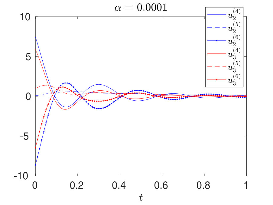 Figure 1
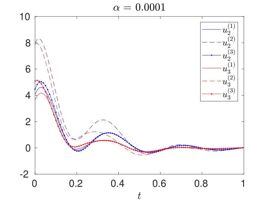 Figure 2
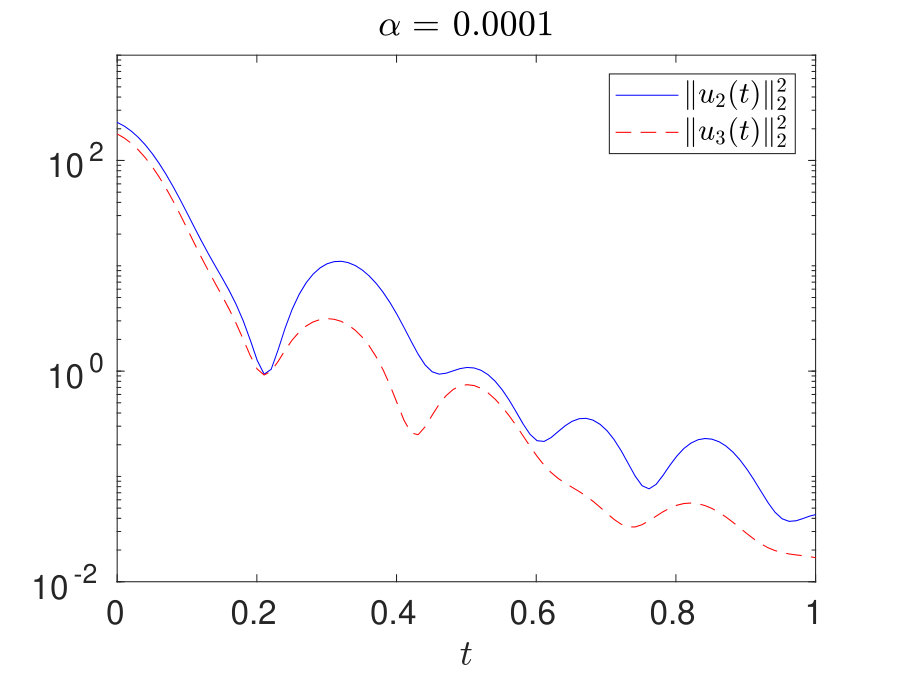 Figure 3
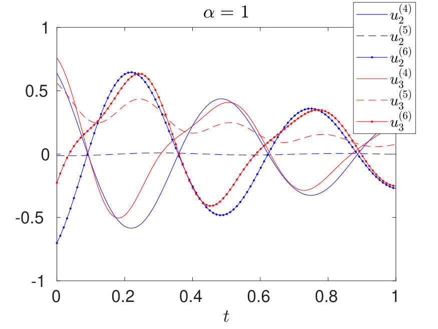 Figure 4
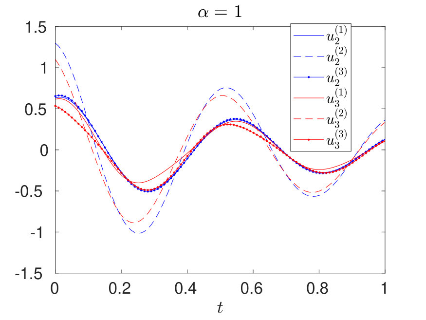 Figure 5
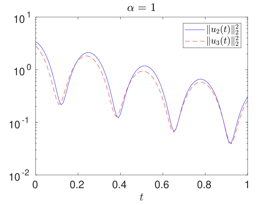 Figure 6
 Figure 7
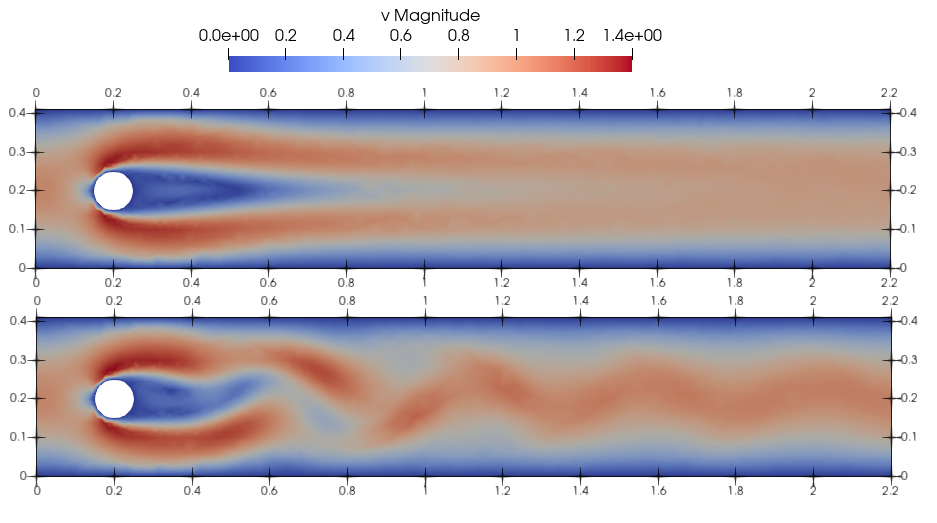 Figure 8
Peer Reviews
No public reviews on file for this paper yet. If you reviewed it on a platform where reviews are public (OpenReview, ICLR, NeurIPS, ICML), you can paste yours below so the community can read it here.
Videos
No videos yet. Explain this paper in a talk, walkthrough, or lecture? Add one.
Feedback Stabilization of the Two-Dimensional Navier-Stokes Equations by Value Function Approximation
Tobias Breiten111Institute of Mathematics, University of Graz, Austria. E-mail: [email protected] Karl Kunisch222Institute of Mathematics, University of Graz, Austria and RICAM Institute, Austrian Academy of Sciences, Linz, Austria. E-mail: [email protected] Laurent Pfeiffer333Institute of Mathematics, University of Graz, Austria. E-mail: [email protected]
Abstract
The value function associated with an optimal control problem subject to the Navier-Stokes equations in dimension two is analyzed. Its smoothness is established around a steady state, moreover, its derivatives are shown to satisfy a Riccati equation at the order two and generalized Lyapunov equations at the higher orders. An approximation of the optimal feedback law is then derived from the Taylor expansion of the value function. A convergence rate for the resulting controls and closed-loop systems is demonstrated.
Keywords: Stabilization, 2-D Navier-Stokes equations, value function, Taylor expansion, feedback control.
AMS Classification: 35Q35, 49J20, 49N35, 93D05, 93D15.
1 Introduction
In this work we continue our investigations of the value function associated with infinite-horizon optimal control problems of partial differential equations, that we initiated in [15, 17]. We consider a stabilization problem of the Navier-Stokes equations in dimension two and focus on the regularity of the value function and its characterization as a solution to a Hamilton-Jacobi-Bellman (HJB) equation. This task has been the subject of tremendous research, for optimal control problems of a general structure, in general associated with finite-dimensional dynamical systems. The use of the notion of viscosity solutions has allowed to deal with the low regularity of the value function. In the present paper, to the contrary, we show that the value function is smooth and that the HJB equation is satisfied in the strict sense, in a neighborhood of the steady state. Moreover, we show that the derivatives of the value function, at the steady state, are solutions to an algebraic Riccati equation (for the order 2) and to linear equations, called generalized Lyapunov equations, for the higher orders. The main interest of these results is the fact that polynomial feedback laws can be derived from Taylor approximations of the value function. Moreover their efficiency can be analyzed.
From a methodological point of view, we mainly follow the techniques that we laid out for bilinear optimal control problems (such as control problems of the Fokker-Planck equation) in [17] and [15]. The Navier-Stokes control system considered here requires a different functional analytic treatment. In fact, the involved nonlinear terms must be tackled with different estimates, to guarantee, for example, the well-posedness of the closed-loop system. They also lead to different generalized Lyapunov equations. Moreover, from the point of view of open-loop control of the Navier-Stokes equation, this paper contains results on infinite-horizon optimal control which are not readily available elsewhere.
Feedback stabilization of the Navier-Stokes equations has been and still is an active topic of research. Among the numerous works, we refer to, e.g., [6, 7, 10, 24, 38], and the references therein. For literature concerning open-loop optimal control of the Navier-Stokes equations, we can only cite a small selection [13, 18, 19, 21, 22, 27, 30, 42].
The technique of approximation of the value function with a Taylor expansion dates back to [3, 35], where optimal control problems associated to finite-dimensional control systems were investigated. We also quote follow-up work, for instance in [2, 8, 36]. For infinite-dimensional problems, we are only aware of [15, 17]. In [16], the numerical solvability of the Lyapunov equations has been addressed. Model reduction techniques based on balanced truncation have been used in this reference to cope with the curse of dimensionality encountered when dealing with PDE controlled systems.
Let us next specify the problem which will be investigated in this paper. Throughout denotes a bounded domain with Lipschitz boundary . Given two vector valued functions and , we consider a solution of the stationary Navier-Stokes equations
[TABLE]
Our goal is to find a control such that the solution to the transient Navier-Stokes equations
[TABLE]
is stabilized around i.e., provided the initial perturbation is small in an appropriate sense. The control operator will be defined below. Throughout this work, we assume that . Our results are concerned with feedback stabilization of (2) and for this purpose, we consider new state variables which satisfy the following generalized Navier-Stokes equations
[TABLE]
The following sections are structured as follows. The problem statement and fundamental results on the state-equation on the time interval are given in Section 2. Section 3 contains the existence theory of optimal controls, the adjoint equation, sensitivity analysis, and differentiability of the value function. The characterization of all higher order derivatives of the value as solutions to generalized Lyapunov equations are provided in Section 4. Section 5 contains the Taylor expansion of the value function, and estimates for convergence rates between the optimal solution and its approximation on the basis of feedback solutions obtained from derivatives of the value function. The paper closes with a very short outlook.
Notation.
For Hilbert spaces with dense and compact embedding, we consider the Gelfand triple where denotes the topological dual of with respect to the pivot space . Given we consider the space
[TABLE]
For , the space will be denoted by . For vector-valued functions , we use the notation . Elements will be denoted in boldface and are distinguished from real-valued functions . Similarly, we use for the space and for . Given a closed, densely defined linear operator in , its adjoint (again considered as an operator in ) will be denoted with .
Let us introduce some notation that will be needed for the description of polynomial mappings. For and a Hilbert space , we denote by the closed ball in with radius and center 0. For , we make use of the following norm:
[TABLE]
Given a Hilbert space , we say that is a bounded multilinear mapping (or bounded multilinear form when ) if for all and for all , the mapping is linear and
[TABLE]
The set of bounded multilinear mappings on will be denoted by . For all and for all ,
[TABLE]
Given a bounded multilinear form and , we denote by the bounded linear form . It will be very often identified with its Riesz representative. Note that
[TABLE]
Bounded multilinear mappings are said to be symmetric if for all and for all permutations of ,
[TABLE]
Finally, given two multilinears mappings and , we denote by the bounded multilinear form defined by
[TABLE]
Throughout the manuscript, we use as a generic constant that might change its value between consecutive lines.
2 Problem formulation
2.1 Abstract Cauchy problem
In this section, we formulate system (3) as an abstract Cauchy problem on a suitable Hilbert space and, subsequently, define the stabilization problem of interest. This procedure is quite standard, see, for instance, [6, 7, 24, 38, 40] for details. We introduce the spaces
[TABLE]
It is well-known that is a closed subspace of . Moreover, we have the orthogonal decomposition
[TABLE]
where
[TABLE]
see, e.g., [40, page 15]. By we denote the Leray projector which is the orthogonal projector in onto . Following, e.g., [6], we define a trilinear form by
[TABLE]
and a nonlinear operator by
[TABLE]
For the bilinear mapping associated with the linearization of , we introduce the operator
[TABLE]
The Oseen-Operator is then defined by
[TABLE]
The following well-known results (see, e.g., [6], [40, Lemma III.3.4]) concerning and will be used frequently throughout the paper.
Proposition 1**.**
The following properties hold for and :
- (i)
, for all ,
- (ii)
, for all .
With the previous result, we obtain similar properties for time-varying functions .
Lemma 2**.**
Let . For all , for all , and for all ,
[TABLE]
Moreover, if ,
[TABLE]
where is the constant given by Proposition 1.
Proof.
Using Proposition 1 and Cauchy-Schwarz inequality (two times), we obtain that
[TABLE]
The two inequalities easily follow. ∎
Corollary 3**.**
There exists such that for all and ,
[TABLE]
For , we further introduce the Stokes-Oseen operator via
[TABLE]
Considered as operator in the adjoint , as operator in , can be characterized by (see, e.g., [38])
[TABLE]
We note that as a consequence of Proposition 1, the operator can be extended to a bounded linear operator from to in the following manner:
[TABLE]
Note that this extension is consistent, since by definition of the Leray projector , we have for all and for all . Similarly, can be extended to a bounded linear operator from to .
The control operator is chosen to satisfy . We further define . The controlled state equation (3) can now be formulated as the abstract control system
[TABLE]
where the pressure is eliminated. We can finally formulate the stabilization problem as an infinite-horizon optimal control problem:
[TABLE]
where and are defined by
[TABLE]
Let us note that is well-defined by Corollary 3.
2.2 Assumptions and first properties
Throughout the article we assume that the following assumptions hold true.
Assumption A1**.**
The stationary solution satisfies .
Assumption A2**.**
There exists an operator such that the semigroup is exponentially stable on .
Assumption A2 concerning the exponential feedback stabilizability of the Stokes-Oseen operator is well investigated. We refer e.g. to [6] where finite-dimensional feedback operators are constructed on the basis of spectral decomposition or alternatively by Riccati theory. In this case A2 can be satisfied with , for appropriately large. Alternatively, we can rely on exact controllability results as obtained in [23]. They imply that the finite cost criterion holds. We can then rely on classical results, see, e.g., [37] which guarantee the existence of a stabilizing feedback operator.
Let us discuss some important consequences of the above definitions and assumptions.
Consequence C1**.**
There exists and such that
[TABLE]
Hence, generates an analytic semigroup on , see [12, Part II, Chapter 1, Theorem 2.12].
Consequence C2**.**
For all , for all , and for all , there exists a unique solution to the system
[TABLE]
This solution satisfies
[TABLE]
with a continuous function . Assuming that , we consider the equivalent equation
[TABLE]
where . By (18), the operator generates an analytic, exponentially stable, semigroup on satisfying for some independent of , see [12, Theorem II.1.2.12]. It follows that and there exists such that with
[TABLE]
This estimate is obtained by adapting [12, Corollary II.3.2.1] and [12, Theorem II.3.2.2] from the temporal domain to , which can be achieved using the exponential stability of .
Lemma 4**.**
There exists a constant such that for all and for all and with and , it holds that
[TABLE]
Proof.
We have
[TABLE]
The assertion now easily follows from Corollary 3. ∎
The following lemma is formulated for an abstract generator of an analytic semigroup on . It will subsequently be used to address the asymptotic behavior of the nonlinear system (15). We point out that the statement is similar to [38, Theorem 6.1] which, since it addresses the boundary control case, assumes a slightly more regular initial condtion .
Lemma 5**.**
Let be the generator of an exponentially stable analytic semigroup on such that (18) holds. Let denote the constant from Lemma 4. Then there exists a constant such that for all and with
[TABLE]
the system
[TABLE]
has a unique solution in , which moreover satisfies
[TABLE]
Proof.
We follow the line of argumentation provided in the proof [38, Theorem 6.1]. Since the semigroup is exponentially stable on , it follows that for all the system
[TABLE]
has a unique solution . Moreover, there exists a constant such that
[TABLE]
Without loss of generality we can assume that . We claim that the constant is the one announced in the assertion. This will be shown by a fixed-point argument applied to the system (20). For this purpose, let us define and let us define the mapping , where is the unique solution of
[TABLE]
If there exists a unique fixed point of , then it is a unique solution of (20) in . With and given, we shall use Lemma 4 with . Together with (21), it follows that
[TABLE]
This implies . For consider now solving
[TABLE]
Again by (21) and Lemma 4 we obtain
[TABLE]
In other words, is a contraction in and therefore, there exists a unique such that . Regarding uniqueness in , consider two solutions . For the difference it then holds
[TABLE]
Multiplying with and taking inner products yields
[TABLE]
Since satisfies an inequality of the form (18), we have
[TABLE]
where and . Using Proposition 1 and Young’s inequality we further obtain
[TABLE]
Taking and sufficiently large, it holds that
[TABLE]
Since and , with Gronwall’s inequality, we conclude that for all . Hence, showing the uniqueness of the solution in . ∎
The following two corollaries are consequences of Lemma 4 and Lemma 5. The constant which is employed is the one given by Lemma 4.
Corollary 6**.**
There exists a constant such that for all and for all with
[TABLE]
there exists a control such that the system
[TABLE]
has a unique solution satisfying
[TABLE]
Proof.
By assumption A2, there exists such that generates an exponentially stable, analytic semigroup on . The result then follows by applying Lemma 5 to the system
[TABLE]
and by defining . ∎
In the following corollary, we assume without loss of generality that the constant given by Consequence C2 is such that .
Corollary 7**.**
Let let be such that the system
[TABLE]
has a solution . If
[TABLE]
then and it holds that
[TABLE]
Proof.
Since , we can apply Lemma 5 to the equivalent system
[TABLE]
where . This shows the assertion. ∎
3 Differentiability of the value function
In this section we perform a sensitivity analysis for the stabilization problem. The main purpose is to analyze the dependence of solutions to () with respect to the initial condition and to show the differentiability of the associated value function, defined by
[TABLE]
3.1 Existence of a solution and optimality conditions
In Lemma 8 we prove the existence of a solution to problem (), assuming that is sufficiently small. We derive then in Proposition 10 first-order necessary optimality conditions.
Lemma 8**.**
There exists such that for all , problem () possesses a solution . Moreover, there exists a constant independent of such that
[TABLE]
Proof.
Let us set, for the moment, , where is as in Lemma 4 and denotes the constant from Corollary 6. Applying this corollary (with ), we obtain that for , there exists a control with associated state satisfying
[TABLE]
where . We can thus consider a minimizing sequence with . We therefore have for all that
[TABLE]
Possibly after further reduction of , we eventually obtain that
[TABLE]
where is as in Corollary 7. It then follows that the sequence is bounded in with . Extracting if necessary a subsequence, there exists such that , and satisfies (23).
Let us prove that is feasible and optimal. For any let us consider an arbitrary . For all , we have
[TABLE]
Since in , we can pass to the limit in the l.h.s. of the above equality. Moreover, since ,
[TABLE]
Analogously, we obtain that
[TABLE]
We also have
[TABLE]
By Lemma 2, it then follows that
[TABLE]
Since is compactly embedded in , we obtain that with the Aubin-Lions lemma. We can pass to the limit in (24) and obtain
[TABLE]
Density of in implies that . Finally, by weak lower semi-continuity of norms it follows that , which proves the optimality of .
Consider now an arbitrary solution to (). It then holds that from which we obtain that
[TABLE]
The estimate (23) for can now be shown by applying the same arguments as above. ∎
For the derivation of the optimality system for () we need the following technical lemma.
Lemma 9**.**
([15, Lemma 2.5]) Let be such that where denotes the operator norm of . Then, for all and , there exists a unique solution to the following system:
[TABLE]
Moreover,
[TABLE]
First-order optimality conditions for finite-horizon optimal control problems have been addressed several times in the literature, we mention e.g. [1, 29, 30, 31]. The finite-horizon case, and in particular the decay properties of the state, the costate, and the optimal control, require independent treatment, which we provide next. For an analysis of the linear infinite-horizon problem, we additionally refer to [38].
Proposition 10**.**
There exists such that for all , for all solutions of (), there exists a unique costate satisfying
[TABLE]
Moreover, there exists a constant , independent of , such that
[TABLE]
Remark 11**.**
Note that (25) is a formal expression for
[TABLE]
where .
Proof of Proposition 10.
Let us set . By Lemma 8, problem () has a solution . In the first part of the proof, we derive abstract optimality conditions, by proving that the mapping (used for formulating the constraints) has a surjective derivative. For proving the differentiability of , we only need to consider the nonlinear term. We have and we know that is a bounded bilinear mapping from to , by Lemma 2. Thus and are Fréchet differentiable, and so is , with
[TABLE]
Let us show that is surjective if is sufficiently small. Let and consider the system
[TABLE]
Observe that by Corollary 3
[TABLE]
By Lemma 8, it further holds that
[TABLE]
For sufficiently small , the operator defined by
[TABLE]
satisfies . By Lemma 9 there exists a unique solution to the system
[TABLE]
Setting proves the surjectivity of . Note that
[TABLE]
for some constant independent of and .
From the surjectivity of and Lagrange multiplier theory it follows that there exists a unique pair such that for all ,
[TABLE]
Using (32) we derive in the second part of the proof the costate equation (25) and relation (26).As can be easily verified, is differentiable with
[TABLE]
Moreover, for all
[TABLE]
Taking and letting vary in , we deduce from (32), (33) and (34) that
[TABLE]
which proves (26). Taking now , we obtain that
[TABLE]
It remains to bound in . Let and let satisfy and the bound (31) (with ). Using the optimality condition (32), the expression (33) of , estimate (31), and estimate (23) on , we obtain the following inequalities:
[TABLE]
Since was arbitrary and since does not depend on , we obtain that . ∎
3.2 Sensitivity analysis
We define a mapping via
[TABLE]
where the third line again has to be understood formally, see Remark 11. We endow the space with the -product norm. The well-posedness of follows from the considerations on and the costate equation (25) that have been given in the proof of Proposition 10.
Lemma 12**.**
There exist , , and three -mappings
[TABLE]
such that for all , the triplet \big{(}\mathcal{Y}(\mathbf{y}_{0}),\mathcal{U}(\mathbf{y}_{0}),\mathcal{P}(\mathbf{y}_{0})\big{)} is the unique solution to
[TABLE]
in . Moreover, there exists a constant such that for all ,
[TABLE]
Proof.
The result is a consequence of the inverse function theorem. Since contains only linear terms and three bilinear terms, it is infinitely differentiable. We also have . It remains to prove that is an isomorphism. Let and let . We have the following equivalence
[TABLE]
It can be proved with the same techniques as for [15, Proposition 3.1, Lemma 4.4] that the linear system on the left-hand side has a unique solution , moreover,
[TABLE]
This proves that is an isomorphism. The inverse function theorem ensures the existence of , , and -mappings , , and with the properties announced in (37).
It remains to prove (38). Reducing if necessary , we can assume that the norms of the derivatives of the three mappings are bounded on by some constant . The three mappings are therefore Lipschitz continuous with modulus . Estimate (38) follows, since \big{(}\mathcal{Y}(0),\mathcal{U}(0),(\mathcal{P}(0)\big{)}=(0,0,0). ∎
Proposition 13**.**
There exists such that for all , the pair is the unique solution to () with initial condition . Moreover, is the unique associated costate.
Proof.
Let us set for the moment. Let . By Lemma 8 and Proposition 10, there exist a solution to () with associated costate which necessarily satisfies
[TABLE]
By further reduction of , we obtain that
[TABLE]
Since , Lemma 12 implies that . The proposition is proved. ∎
Corollary 14**.**
The value function is infinitely differentiable on .
Proof.
The cost function is clearly infinitely differentiable. Since , is then the composition of infinitely differentiable mappings, which shows the assertion. ∎
3.3 Additional regularity for
We next assert that for small initial data the adjoint state is more regular than . For this, we need more smoothness of the boundary .
Assumption A3**.**
Let denote a bounded domain with smooth boundary .
Proposition 15**.**
There exists such that for all , for all solutions of (P), there exists a unique costate satisfying
[TABLE]
Moreover, there exists a constant , independent of , such that
[TABLE]
The proof is given in the appendix.
4 Derivatives of the value function
By standard arguments, we can derive a Hamilton-Jacobi-Bellman equation which provides an optimal feedback control based on the derivative of the value function.
All along the section, the first-order derivative is either seen as a linear form on or is identified with its Riesz representative in . The identification is done for example in the term appearing in the HJB equation below.
Proposition 16**.**
There exists such that for all , the following Hamilton-Jacobi-Bellman equation holds:
[TABLE]
Moreover,
[TABLE]
where
Remark 17**.**
Note that by, e.g., [6, Proposition 1.7], we have that and, as a consequence, the term is well-defined.
Proof.
Let us set . Let . Let us consider the Hamiltonian of the system, defined by
[TABLE]
Using the arguments provided in the proof of [17, Proposition 9], one can prove that
[TABLE]
from which (42) derives. One can also prove that
[TABLE]
which proves (43) for . Let us emphasize that the assumptions which are required in [17, Proposition 9] are satisfied. In particular, the optimality condition which holds in implies that is almost everywhere equal to a continuous function. We can thus assume that is continuous. For proving (43) for all , one has first to reduce so that , for all . For a given , we have by dynamic programming that is the solution to () with initial condition and thus (43) holds true at . ∎
For deriving a Taylor series expansion of , let us follow the approach from [3] and differentiate (42) in some direction . To alleviate the calculations, we denote the variable in (42) by . We then obtain
[TABLE]
A second differentiation in the directions yields the equation
[TABLE]
Since and for all , it follows that . We can thus evaluate the last equation for to obtain
[TABLE]
We recall that is a bounded and symmetric bilinear form on and thus can be represented (see, e.g., [32, Chapter 5, Section 2]) by an operator such that
[TABLE]
As a consequence, we can formulate (44) as
[TABLE]
Equation (45) is the well-known algebraic operator Riccati equation which has been studied in detail in, e.g., [20, 33]. From the stabilizability assumption A2, and the fact that the pair is exponentially detectable as a consequence of (18), we conclude that (45) has a unique stabilizing solution . In the discussion below, we denote by
[TABLE]
the closed-loop operator associated with the linearized stabilization problem. In particular, let us mention that generates an analytic exponentially stable semigroup on . Hence, for trajectories of the form , it follows that .
For higher order derivatives of , we follow the exposition from [17]. For this purpose, let us briefly recall the symmetrization technique introduced there. Let and , consider
[TABLE]
where is the set of permutations of . A permutation is uniquely defined by the subset , therefore, the cardinality of is equal to the number of subsets of cardinality of , that is to say . For a multilinear mapping of order , we set
[TABLE]
The following proposition is a generalization of the Leibniz formula for the differentiation of the product of two functions.
Proposition 18**.**
Let be a Hilbert space. Let and be two -times continuously differentiable functions. Then, for all , for all and ,
[TABLE]
Proof.
The proof is analogous to the one given in [17, Lemma 10] for . ∎
Theorem 19**.**
Let . For all ,
[TABLE]
where the multilinear form is given by
[TABLE]
with and .
Proof.
The proof relies on successive differentiations of (42). For a bilinear control problem, a similar result has been obtained in [17, Theorem 12]. In particular, it was shown that
[TABLE]
Obviously, for , we have . Let us discuss the structure of the derivatives of the remaining terms appearing in (42). Applying Proposition 18 to the term , we obtain
[TABLE]
Since has a minimum at the origin, we have and the terms for and vanish when evaluated in . By definition of the -operator, for we obtain
[TABLE]
As explained previously, we can represent in terms of the solution of the algebraic operator Riccati equation. This shows
[TABLE]
A similar relation can be derived for . Finally we consider the term . By Proposition 18, we get
[TABLE]
Since for all , the previous equation simplifies as follows
[TABLE]
Evaluating the last expression in yields
[TABLE]
since and are both null. Combining (48), (49) and (50) proves the assertion. ∎
5 Polynomial feedback laws
5.1 Estimates for the velocity
In this section we analyze the polynomial feedback law derived from the Taylor series approximation of the value function
[TABLE]
for a given . The feedback is obtained by approximating with in formula (43), that is
[TABLE]
The associated closed-loop system is given by
[TABLE]
Below we will also derive an estimate for the open-loop control, i.e., the function defined by
[TABLE]
which is obtained via closed-loop dynamcics here. With slight abuse of notation, the open-loop control as well as its closed-loop interpretation will both be denoted with .
We begin with some local Lipschitz continuity estimates for the nonlinear part of the feedback law. For this purpose, we set
[TABLE]
for all . The closed-loop system can be reformulated as follows:
[TABLE]
Lemma 20**.**
For all , there exists a constant such that for all and ,
[TABLE]
Moreover, for all , for all and such that and ,
[TABLE]
Proof.
We have the identity
[TABLE]
The first inequality easily follows, with and as defined in (5). We also obtain that for all and ,
[TABLE]
The second inequality follows, since and . ∎
The well-posedness of the closed-loop system can be now established with the same tools as those used in Lemma 5.
Theorem 21**.**
Let . Let and denote the constants from Lemma 4 and Lemma 20. There exists a constant such that for all with
[TABLE]
the closed-loop system (51) has a unique solution in , which satisfies
[TABLE]
Proof.
The existence of a solution , satisfying (55), can be obtained exactly as in Lemma 5. Thus we only discuss uniqueness. Let and denote two solutions to (51) in . Let us set . Arguing as in the proof of Lemma 5, one can prove the existence of such that
[TABLE]
for all . Since and and , we obtain with Gronwall’s inequality that , which proves the uniqueness of the solution to the closed-loop system. ∎
Theorem 22**.**
Let . There exist and such that for all , it holds that
[TABLE]
where , is the solution of the closed-loop system (51) with initial condition , and is as defined in (52).
Proof.
Let us fix \delta_{6}=\min\big{(}\delta_{5},(4(C+\sum_{k=3}^{d}C(k))M_{\text{cls}}^{2})^{-1}\big{)}, so that Proposition 16 and Theorem 21 apply for . By Taylor’s theorem, see, e.g., [43, Theorem 4A], there exists such that for all ,
[TABLE]
where the remainder term satisfies
[TABLE]
for some constant independent of . Reducing if necessary , we have that for all . Combining then (43) and the Taylor expansion (56), we obtain that
[TABLE]
Let us now consider the error dynamics . We have , moreover by (54) and (57),
[TABLE]
Alternatively, can be expressed as the solution of the system
[TABLE]
where the source term is given by
[TABLE]
Consider . The precise value of will be fixed later. By Lemma 12 and Theorem 21, we can reduce so that . We first observe that
[TABLE]
Applying further Lemma 4 and Lemma 20, we obtain
[TABLE]
For the solution of system (58) we thus obtain the estimate
[TABLE]
The constant in the above estimate is independent of . We can now define \tilde{\delta}=\min\big{(}1,\frac{1}{2M}\big{)}. The first estimate on follows.
Let us estimate . By (43) and by definition of the generated open-loop control , we have that
[TABLE]
Let us estimate the two terms of the right-hand side. It is easy to check that
[TABLE]
Using the techniques of Lemma 20 and the estimate on , we also obtain that
[TABLE]
The second estimate on follows. ∎
5.2 Estimates for the pressure
It is well-known that for , the pressure term that can be associated to the Navier-Stokes equations is a distribution only (see, e.g., [39], [40, Chapter III-§3]). In the following, we redemonstrate this fact and we argue that a result analogous to Theorem 22 also holds for the pressure, provided the latter is considered in with
[TABLE]
and
[TABLE]
We define similarly . We recall here that embeds continuously into . Further the elements of can be identified a.e. with continuous functions on and satisfy . We use the properties of Banach-space valued functions as summarized in [14, Chapter II-§5].
Lemma 23**.**
Let be such that . Then, there exists a unique such that
[TABLE]
that is,
[TABLE]
for all . Moreover,
[TABLE]
for a constant independent of .
Proof.
We follow the technique consisting in integrating the state equation, see, e.g., [14, Chapter V-§1] and introduce
[TABLE]
It can be easily shown that and that there exists a constant independent of such that
[TABLE]
This estimate can be obtained with the Cauchy-Schwarz inequality and Proposition 1(i), which also holds true in (in place of ). Since , it further follows that is a continuous function of time with values in . Moreover, for all and . Hence for all , there exists a unique such that , see, e.g., [14, Theorem IV.2.3]. Let us prove that . Recall first that there exists an operator with the property that
[TABLE]
see [14, Theorem IV.3.1]. Let be arbitrary and let . For all and in , we have
[TABLE]
It follows that , which concludes the proof of continuity of . We now introduce the distributional derivative and establish that . Let be arbitrary and set . Note that . We have
[TABLE]
Recalling the embedding of in , we deduce that
[TABLE]
Using then estimate (62), we obtain that can be extended to an element of satisfying estimate (60).
With the same calculations as above, we can show that for all ,
[TABLE]
which proves that satisfies (59). Let us prove the uniqueness. Let satisfy (59). Let be arbitrary and let us set . Then, by (59), we have
[TABLE]
which proves that and concludes the proof. ∎
We have the following result, extending Theorem 22.
Proposition 24**.**
Let . There exists such that for all with ,
[TABLE]
where and denote the pressure terms associated with and respectively.
Proof.
We have introduced in the proof of Lemma 23 the term associated with a feasible pair . Let us denote by and the corresponding terms associated with and . One can verify that as a consequence of Theorem 22, . Proposition 24 follows then with similar calculations to those performed in the proof of Lemma 23. ∎
6 A numerical example
In this section, we present numerical simulations for the two-dimensional Navier-Stokes equations and computed feedback laws of order 2 and 3. The discretization procedure and the example setups are classical and are taken from [9]. The main purpose is to show that the computation of higher order feedback laws is possible and, depending on the chosen parameters, visible differences to a Riccati-based feedback law can be observed.
6.1 Setup and discretization
We briefly summarize the numerical implementation provided in [9]. Therein a Taylor-Hood - finite element discretization for a two dimensional wake behind a cylinder is discussed. The computational domain as well as a non uniform grid are shown in Figure 1. For all simulations, we use the Reynolds number and the parabolic inflow profile discussed in [9].
For the upper and lower end of the geometry, no slip boundary conditions are employed. The outflow is modeled by do nothing boundary conditions on the right end of the geometry. For the desired stabilization, we utilize a distributed, separable control acting in the control domain . In particular, the control operator is of the form
[TABLE]
where the control shape functions and are piecewise linear functions which are constant along the -direction.
The finite element discretization is computed in FEniCS and the resulting matrices associated with the spatial semidiscretization are exported to MATLAB. As described in detail in [9], the (spatially) discrete system takes the form
[TABLE]
where are the mass and stiffness matrices, represents the discrete divergence operator, the tensor matricization represents the trilinear form (9) and is the discrete control operator. Note that can be constructed in such a way that for any . The time invariant vectors and are due to the elimination of the boundary nodes. The following results correspond to a discretization level with and . The velocity profile of the unstable steady state solution shown in Figure 2 is obtained by a Picard iteration applied to the uncontrolled stationary system, i.e., system (63) with and . To illustrate that the controller stabilizes this steady state solution, we start the transient simulations of the closed-loop systems from the slightly randomly perturbed steady state .
6.2 Reformulation as an ODE system
System (63) is a system of differential-algebraic equations (DAEs) and hence the results from above are not readily applicable. While a thorough analysis in the framework of control of DAEs is certainly of interest, at this point we employ a reformulation initially proposed in [28] that allows to rewrite the dynamics as a set of ODEs for the velocity vector . As in (3), we consider the shifted variables and , respectively. Consequently, we obtain
[TABLE]
where . Let us note that the second equation implies . Following [28, Section 3], from the first equation, we thus obtain
[TABLE]
We can now eliminate the pressure from (64) using the relation
[TABLE]
With the notation this yields the system
[TABLE]
In fact, as has been discussed in [11], the matrix as a discrete realization of the Leray projector. Since , we have so that we can multiply the last equation by to obtain
[TABLE]
Finally, by means of a decomposition with we can project onto the dimensional subspace and arrive at the ODE system
[TABLE]
where . For the initialization, we use . At this point, we emphasize that the explicit formulas yield dense matrices and thus are rather a theoretical tool. In particular, an explicit computation of is infeasible for the problem dimension considered here. As a remedy, we work with an implementation that applies the above operations whenever a matrix vector multiplication is needed.
6.3 Computing the feedback gain
With the previous considerations in mind, we focus on the stabilization problem
[TABLE]
where
[TABLE]
We illustrate the effect of higher order feedback laws by computing the first two non trivial derivatives and , respectively. For the computation of , we have to solve the algebraic matrix Riccati equation
[TABLE]
which in our case was done by means of the MATLAB function care. For the third order tensor we have to solve a linear system of the form where
[TABLE]
where denotes the vectorization of and the permutation matrix is given by
[TABLE]
Let us emphasize that is the discrete realization of the term in (47). In particular, the tensor is symmetric. Note that computing a solution to is infeasible without using further tools such as model order reduction or tensor calculus as storing the vector already requires more than TB of data. As a remedy, we aim for a direct computation of the corresponding feedback gain
[TABLE]
without explicitly computing . With this in mind, we proceed as in [16] and utilize a quadrature-based approximation that has been analyzed in [25]. From [25, Lemma 3], it follows that
[TABLE]
As shown in [25, Theorem 9], the previous integral can be well approximated by a tensor sum of the form
[TABLE]
where and are suitable quadrature points and weights and denotes a constant determined by the spectrum of the matrix pencil . Combining the representation in (67), (68) and (69), we obtain the following approximation formula for the feedback gain
[TABLE]
with in the numerical examples. By use of algebraic manipulations such as reshaping and transposition of matrices, the computation of the permutation matrix as well as computation of the dense matricization can be avoided. As a consequence, we obtain an approximation of whose storage requires less than 4 GB of data. Let us point out that the above considerations do not fully break the curse of dimensionality but nevertheless allow us to compute a third order feedback law even for a spatially discretized PDE. For the simulation of the time-varying systems, we make use of the MATLAB function ode23 with the standard relative error tolerance . In each time step, the control laws and are obtained via
[TABLE]
where denotes the identity matrix for the control space .
6.4 Results
Below, we present a numerical comparison for two different values of . In Figure 3, the control laws corresponding to (66) with are shown. We observe that both feedback laws and , respectively, exhibit a similar behavior and create vortices which induce the desired control. Indeed, the control velocities in -direction are of opposite sign (with the centered velocitiy field being negligible) while the control velocities in -direction all have the same sign.
For , Figure 4 shows more visible differences between the control laws.
It would certainly be of interest to investigate the numerical convergence behavior as the order of the control laws increases. At the moment, however this is out of reach, and could be based on model reduction techniques in an independent numerical endeavor. In Figure 4, we observe that the amplitudes of the controls decay more rapidly than those of the controls. This is consistent with Figure 5, where we compare the dynamical behavior of and . Let us emphasize that for , for all , the norm of the control law is smaller than the one of . For the values of the cost functionals, we obtain
[TABLE]
which indicates that higher order feedback laws can be of interest for feedback stabilization.
7 Outlook
In the present paper we demonstrated that the approach that we carried out for obtaining Taylor approximations to the value function of optimal control problems related to the Fokker-Planck equation, is also applicable for optimal control of the Navier-Stokes equations in dimension two. The question arises to which extent analogous results can be obtained for dimension three and for boundary control problems. In dimension three the situation will be significantly different from that of the current paper. It will not be possible to work with weak variational solutions. Rather one has to resort to strong variational solutions, and thus one can expect at best that the value function is smooth on rather than on . This leads to difficulties for the operator representations of the derivatives of the value function. Alternatively one can start by analyzing (47) as equations for abstract multilinear forms , which are not necessarily obtained of derivatives of . This is an approach which we plan to follow.
Acknowledgement
This work was partly supported by the ERC advanced grant 668998 (OCLOC) under the EU’s H2020 research program. The authors would like to thank Jan Heiland for making available his finite element based code for solving the state equation as well as many helpful and interesting discussions on the numerical examples.
Appendix A Appendix
The appendix is dedicated to the proof of Proposition 15.
We follow the notation from, e.g., [5] and define the following spaces
[TABLE]
Moreover, we consider where is the Stokes-Oseen operator and is such that generates an exponentially stable and contractive semigroup on . From [5, Theorem 20], let us recall that
[TABLE]
While not needed for our purposes, let us emphasize that the case is also included in [5, Theorem 20].
Using the above notation, for let us consider the space
[TABLE]
As mentioned in, e.g., [4], it holds that
[TABLE]
From [34, Theorem 4.2], we thus conclude that
[TABLE]
where denotes the space of continuous and bounded functions.
Before we continue, let us cite the following result from [26].
Proposition 25**.**
([26, B.1]) Let . One has for and (where is a smooth open subset of ):
[TABLE]
- (i)
when ,
- (ii)
with
- (iii)
except that if equality holds somewhere in .
These estimates allow us to bound the coupling terms appearing in the adjoint equation.
Lemma 26**.**
Let . Let and Then
[TABLE]
Proof.
For the first assertion, consider with . Set . Then
[TABLE]
Applying Proposition 25 with and yields
[TABLE]
which shows the first statement. For the second statement, set , , and . ∎
The following lemma is formulated for an abstract generator of an analytic exponentially stable semigroup on . It will subsequently be applied with .
Lemma 27**.**
Let generate an exponentially stable semigroup on and assume that there exists such that for every there exists a unique satisfying
[TABLE]
Then there exists such that for all there exists a unique such that
[TABLE]
Proof.
Step 1. Let us define by . Considering the adjoint we have:
[TABLE]
Since, by assumption, is a homeomorphism it is in particular surjective and injective and by the closed range theorem there exists a constant such that
[TABLE]
Step 2. Let be arbitrary. Then there exists a unique such that , and by (70) we have Since we have for all
[TABLE]
This implies that the time derivative of , in the sense of distributions, can be extended to a linear form on with the formula:
[TABLE]
We estimate
[TABLE]
Together with (71) and recalling that is dense in , we obtain that can be extended to a bounded linear form on , i.e., can be extended to an element of , moreover,
[TABLE]
It follows that . Moreover,
[TABLE]
∎
Corollary 28**.**
Let For all , the system
[TABLE]
has a unique solution . Moreover, there exists a constant independent of such that
[TABLE]
Proof.
We appy Lemma 27 to with , to obtain . Setting and using that is an isomorphism from to and from to , [41, Section 1.15.2, p.101], the claim follows.
∎
Proof of Proposition 15.
Only regularity has to be shown. Let us fix and let be given by Corollary 28. Let us define
[TABLE]
Let us then choose such that
[TABLE]
where and are given by Lemma 26. Further consider the mapping defined by
[TABLE]
where is the unique solution of
[TABLE]
according to Lemma 26 and Corollary 28. Given , it holds that
[TABLE]
We obtain that . Consider and let . Note that solves
[TABLE]
so that we obtain
[TABLE]
Thus by the Banach fixed point theorem we conclude that there exists which is a solution of
[TABLE]
It remains to show that solves (25). For this, we define and observe that satisfies
[TABLE]
where the operator is defined in (30). It follows from (70) that
[TABLE]
As a consequence of (29), can be reduced so that . Hence, we obtain and thus showing that . ∎
The reference list from the paper itself. Each links out to its DOI / PubMed record.
- 1[1] F. Abergel and R. Temam , On some control problems in fluid mechanics , Theoret. Comput. Fluid Dynamics, 1 (1990), pp. 303–325.
- 2[2] C. O. Aguilar and A. J. Krener , Numerical solutions to the Bellman equation of optimal control , Journal of Optimization Theory and Applications, 160 (2014), pp. 527–552.
- 3[3] E. Al’brekht , On the optimal stabilization of nonlinear systems , Journal of Applied Mathematics and Mechanics, 25 (1961), pp. 1254–1266.
- 4[4] M. Badra , Abstract settings for stabilization of nonlinear parabolic system with a Riccati-based strategy. application to Navier-Stokes and Boussinesq equations with Neumann or Dirichlet control , Discrete & Continuous Dynamical Systems - Series A, 32 (2012), pp. 1169–1208.
- 5[5] M. Badra and T. Takahashi , Stabilization of parabolic nonlinear systems with finite dimensional feedback or dynamical controllers: Application to the Navier-Stokes system , SIAM J. Control Optim., 49 (2011), pp. 420–463.
- 6[6] V. Barbu , Stabilization of Navier-Stokes Flows , Communications and Control Engineering Series, Springer, London, 2011.
- 7[7] V. Barbu, I. Lasiecka, and R. Triggiani , Tangential boundary stabilization of Navier–Stokes equations , Memoirs of the American Mathematical Society, 181 (2006), pp. 1–128.
- 8[8] S. Beeler, H. Tran, and H. Banks , Feedback control methodologies for nonlinear systems , Journal of Optimization Theory and Applications, 107 (2000), pp. 1–33.