Offset errors in probabilistic inversion of small-loop frequency-domain electromagnetic data: a synthetic study on their influence on magnetic susceptibility estimation
Christin Bobe, Ellen Van De Vijver

TL;DR
This study investigates how systematic offset errors in small-loop frequency-domain electromagnetic data affect the estimation of magnetic susceptibility, demonstrating that joint estimation of offsets improves inversion accuracy.
Contribution
It introduces a probabilistic inversion method that jointly estimates measurement offsets along with subsurface properties, enhancing susceptibility estimation accuracy.
Findings
Joint offset and property estimation reduces bias in susceptibility results.
Using multiple measurement heights improves offset correction.
Systematic errors significantly impact magnetic susceptibility estimates.
Abstract
Small-loop frequency-domain electromagnetic (FDEM) devices measure a secondary magnetic field caused by the application of a stronger primary magnetic field. Both the in-phase and quadrature component of the secondary field commonly suffer from systematic measurement errors, which would result in a non-zero response in free space. The in-phase response is typically strongly correlated to subsurface magnetic susceptibility. Considering common applications on weakly to moderately susceptible grounds, the in-phase component of the secondary field is usually weaker than the quadrature component, making it relatively more prone to systematic errors. Incorporating coil-specific offset parameters in a probabilistic inversion framework, we show how systematic errors in FDEM measurements can be estimated jointly with electrical conductivity and magnetic susceptibility. Including FDEM…
Click any figure to enlarge with its caption.
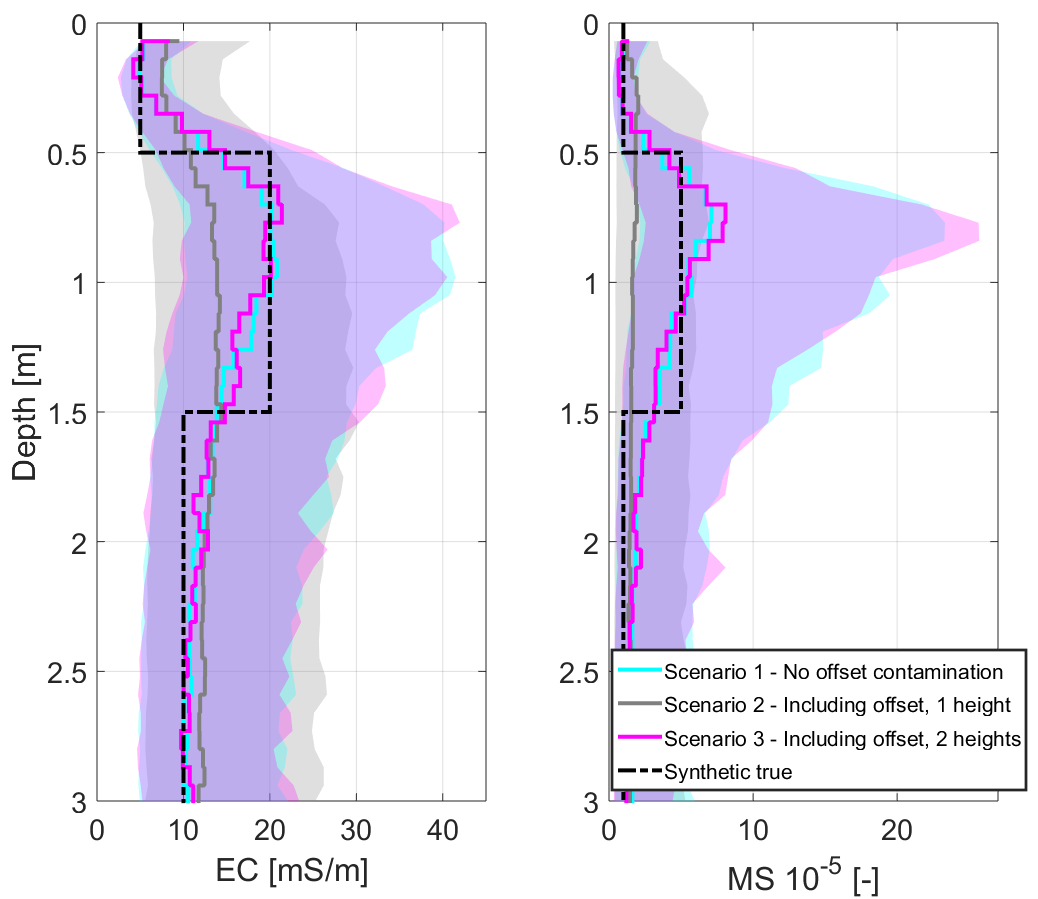 Figure 1
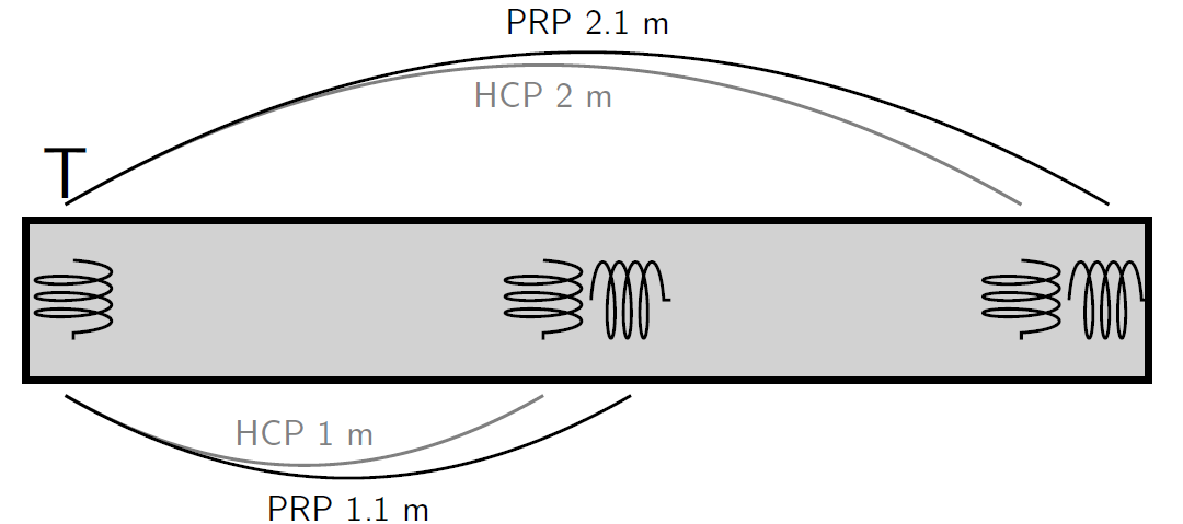 Figure 2
| Quadrature-phase [ppm] | |||||
|---|---|---|---|---|---|
| Prior offset | |||||
| 0.2 m | 1.0 m | True Offset | mean | STD | |
| HCP 1 m | 183.61 | 85.60 | 13.00 | 18.00 | 3.00 |
| PRP 1.1 m | 129.18 | 27.96 | -100.00 | -180.00 | 30.00 |
| HCP 2 m | 832.36 | 550.23 | 24.00 | 22.00 | 5.00 |
| PRP 2.1 m | 724.37 | 272.41 | -19.00 | -22.00 | 5.00 |
| In-phase [ppm] | |||||
| HCP 1 m | 2.99 | 1.93 | 19.00 | 12.00 | 3.00 |
| PRP 1.1 m | -10.13 | -1.23 | -17.00 | -12.00 | 3.00 |
| HCP 2 m | 36.82 | 23.63 | 20.00 | 20.00 | 5.00 |
| PRP 2.1 m | -12.00 | -5.03 | -21.00 | -20.00 | 5.00 |
| Quadrature-phase [ppm] | |||
|---|---|---|---|
| True | Scenario 2 | Scenario 3 | |
| HCP 1 m | 13.00 | 10.21 1.38 | 13.23 0.72 |
| PRP 1.1 m | -100.00 | -115.22 5.41 | -100.04 0.07 |
| HCP 2 m | 24.00 | 26.05 4.90 | 26.10 5.70 |
| PRP 2.1 m | -19.00 | 19.91 4.71 | -19.32 0.39 |
| In-phase [ppm] | |||
| HCP 1 m | 19.00 | 14.20 1.89 | 19.21 0.34 |
| PRP 1.1 m | -17.00 | -18.32 1.66 | -16.95 0.07 |
| HCP 2 m | 20.00 | 12.31 3.71 | 21.47 2.56 |
| PRP 2.1 m | -21.00 | -29.87 1.66 | -20.79 0.27 |
Peer Reviews
No public reviews on file for this paper yet. If you reviewed it on a platform where reviews are public (OpenReview, ICLR, NeurIPS, ICML), you can paste yours below so the community can read it here.
Videos
No videos yet. Explain this paper in a talk, walkthrough, or lecture? Add one.
\setcapindent
0em
Offset errors in probabilistic inversion of small-loop frequency-domain electromagnetic data: a synthetic study on their influence on magnetic susceptibility estimation
Christin Bobe Ellen Van De Vijver
Department of Environment Corresponding Author: [email protected], Department of Environment, Ghent University, Gent, Belgium
Ghent University
Gent
Belgium
Abstract
Small-loop frequency-domain electromagnetic (FDEM) devices measure a secondary magnetic field caused by the application of a stronger primary magnetic field. Both the in-phase and quadrature component of the secondary field commonly suffer from systematic measurement errors, which would result in a non-zero response in free space. The in-phase response is typically strongly correlated to subsurface magnetic susceptibility. Considering common applications on weakly to moderately susceptible grounds, the in-phase component of the secondary field is usually weaker than the quadrature component, making it relatively more prone to systematic errors. Incorporating coil-specific offset parameters in a probabilistic inversion framework, we show how systematic errors in FDEM measurements can be estimated jointly with electrical conductivity and magnetic susceptibility. Including FDEM measurements from more than one height, the offset estimate becomes closer to the true offset, allowing an improved inversion result for the subsurface magnetic susceptibility.
Accepted for publication in International Workshop on Gravity, Electrical and Magnetic Methods and Their Applications (GEM) 2019 Xi’an. Copyright (2019) Society of Exploration Geophysicists (SEG) and Chinese Geophysical Society (CGS). Further reproduction or electronic distribution is not permitted.
1 Introduction
Electrical conductivity (EC) and magnetic susceptibility (MS) determine frequen-cy-domain electromagnetic measurements (FDEM). Using small-loop sensors, secondary field responses are usually small compared to the present primary field. Small measurement quantities are particularly sensitive to systematic calibration errors. These errors imply that a hypothetic free-space measurement would yield non-zero results Sasaki et al., (2008). Therefore, one way of calibration is to quantify the offset error by performing a measurement far from any conductive matter. Unfortunately, this is often practically infeasible. Alternatively, the offset is often corrected by repeated measurements on multiple elevations above ground, including the offset as an additional parameter in an inversion of such data, under the assumption that the offset is constant. This procedure has been proven to result in more reliable estimates for subsurface EC (e.g., Sasaki et al., (2008) and Tan et al., (2018)).
However, the aforementioned studies focus on EC and do not include inversion for subsurface MS. The FDEM in-phase response usually shows a strong correlation to subsurface MS, but, is often smaller than its quadrature counterpart and therefore even more prone to offset errors. For that reason, the in-phase response is often not used in inversion for EC. We show, using a synthetic example, how multi-elevation measurements from multi-coil measurement setups can be used to derive reliable MS inversion results and an estimation for offset errors. The synthetic subsurface model consists of three horizontal layers, including variation in EC as well as in MS. FDEM responses for this subsurface are simulated using a one-dimensional solution to Maxwell’s equations Ward and Hohmann, (1988). Applying the Kalman ensemble generator Nowak, (2009) for inversion of the simulated FDEM responses, we perform a probabilistic inversion, approximating probability distributions by an ensemble of subsurface realizations.
Similar to former studies (e.g., Sasaki et al., (2008) and Tan et al., (2018)), we add constant offset errors for each receiver coil as parameters in the inversion framework. The probabilistic framework allows to jointly estimate EC, MS and the offset errors. Unlike to the method proposed by Sasaki et al., (2008), we do not introduce further regularization to an iterative inversion process. Instead, the offset is estimated through a search of the prior model parameter space, resulting in an offset estimate including uncertainty. For our synthetic study, we will give offset priors where only in one case the true offset matches the prior mean.
The advantage of multiple elevations for a FDEM measurement inversion is demonstrated by comparing the result to an inversion in which only measurements from one height are considered. Finally, both results are compared to the inversion result for a data set without offset errors.
2 Forward simulation
The synthetic FDEM data are simulated using a one-dimensional forward model, allowing for vertical variation of EC and MS (Ward and Hohmann, (1988), and Hanssens et al., (2019)). In small-loop systems, a primary field is computed by assuming an alternating current in a transmitter coil. A secondary field is simulated based on induction currents in conductive model layers. The simulated measurement quantity is the field strength as registered by the induced voltage in a receiver coil at a defined model position with respect to the transmitter coil. In the following, the secondary field is expressed in parts-per-million (ppm) of the primary field. The offset error is included in the forward model by shifting the responses by a constant value.
3 Inversion method
The previously described forward model, in the following called , also serves as the kernel for the probabilistic Kalman ensemble generator inversion (KEG; Nowak, (2009)). A full publication on this FDEM inversion procedure is currently under review with moderate revisions. In this probabilistic framework, we seek a posterior probability distribution for the inversion parameters given FDEM measurements . According to EC and MS for each discretized layer and a coil specific offset, the forward responses are computed:
[TABLE]
Inserting the true physical parameters in , we derive the synthetic measurements . Using Bayes theorem, one derives the posterior probability solving
[TABLE]
with a normalization constant Allmaras et al., (2013). The likelihood , for measurements given a set of parameters , is computed by comparing to (assuming a noise-free for the synthetic data). The prior information on the Gaussian parameters is given by (see below).
As mentioned above, for solving equation 2, we apply the KEG as introduced by Nowak, (2009), a stationary implementation of the widely used Ensemble Kalman filter (EnKF; Evensen, (2003)). The advantage of using a probabilistic approach to inversion lies in the simplicity of including the offset error as estimated parameter, and in the availability of an uncertainty estimate. The EnKF is an ensemble approximation to the original Kalman filter Kalman, (1960). In EnKF, Gaussian probability density functions (PDFs) for model parameters are characterized by random samples drawn from these PDFs. These random samples are single model realizations which are combined in an ensemble matrix , for which is computed and stored in the response matrix . Incorporating random noise as standard deviation (STD) to the FDEM measurements for all coils, also here samples are drawn to derive the data matrix . The inversion update is derived from the matrix equation Evensen, (2003)
[TABLE]
where the primed matrices mean that the mean value of each column is subtracted from this column.
Prior information
The number of inversion parameters is determined by (1) the number of discrete subsurface layers, to which we assign EC and MS values, and (2) the number of coils, to each of which we assign offsets for both the in-phase and the quadrature-phase measurements. To all parameters we attribute prior information through definition of their prior PDFs. To enforce positive values of EC and MS, we use log-normal distributions that are transformed to normal distributions before the update step.
To exclude spurious detail and limit the influence of the prior model, we restrict the prior to a model with uniform mean and STD for all discrete layers. The uniform prior is derived from Gauss sampling, i.e. mean and STD for EC and MS are derived considering 10 cm intervals of the synthetic true.
When no geological layer boundary is present, electric and magnetic properties of adjoining layers will be similar. A simple covariance matrix is introduced in which only the diagonal and the first off-diagonals are filled with non-zero values. On the diagonal, we write the variance of the expectations , on the first off-diagonals we include a value smaller than variance as correlation between the layers (half of the variance in our case). Finally, the prior model is described as a multivariate Gaussian .
The prior offsets shall be updated independently for each coil and each in-phase and quadrature component. Hence, no correlation is introduced in between offset parameters. Moreover, no logarithmic barrier is introduced here since the offset is assumed to take positive as well as negative values (often dependent on the specific coil geometry).
Inversion result
The Gaussian posterior is derived by computing the mean and the STD of the ensemble realizations for all parameters in . We consider the mean as the best fit to the measurement data, while the standard deviation is considered as its corresponding uncertainty. The Gaussianity of the posterior is enforced by the KEG method, such that the derived uncertainty information can only be considered unbiased when the forward solutions around do not deviate too strongly from linearity.
4 Synthetic example
The synthetic example consists of a subsurface including three horizontal layers, varying in EC as well as in MS (synthetic true shown in Figure 2). The simulated FDEM measurement setup consists of one transmitter coil and four receiver coils (Fig. 1). Two receiver coils are in a horizontal co-planar (HCP) configuration, the two other receivers in a perpendicular (PRP) configuration. Measurements are simulated at two height above ground, at 0.2 m and 1 m (Table 1).
Using the outlined KEG inversion, we compare three scenarios. Scenario 1 uses the inversion as described above, but without including offset parameters, i.e. using data simulated at one height (0.2 m) that are not contaminated with an offset shift. This is considered the benchmark for the other two scenarios. For scenarios 2 and 3, data was shifted with an offset as listed in Table 1. For scenario 2, we only consider measurement data from 0.2 m (Table 1) height. Scenario 3 uses additional simulated measurements at 1 m height. Thus, twice as many measurements are used in deriving the inverse model.
Another plausible scenario is not considered in this manuscript: using measurements contaminated by offset shifts yet not include the offset in the inversion parameters. Such a scenario leads to unphysical updates, since the measurement data are inherently inconsistent. The inconsistency is caused by the fact that the offset remains constant, while the measurement response gets weaker as the instrument is lifted.
For EC, MS and the offset, identical prior models are chosen for all investigated scenarios – except for the offset prior in scenario 1, since there is no offset in this scenario. Inverse model layers have a thickness of 0.07 m. The STD for the FDEM data matrix are set to a negligibly small value of 0.05 ppm, expressing that the simulated measurements are considered to be noise free. We sample the prior PDFs creating an ensemble of 10,000 model realizations.
Except for the HCP 2m coil in-phase response, the chosen prior mean values are not identical to the true offset. For the quadrature component of the PRP 1.1 m coil, a large offset is given. It is also noted that the true offset is not within one STD of the prior model.
The results for the offset estimation are listed in Table 2. The corresponding inversion results for both EC and MS for all scenarios are shown in Figure 2. The best fit offset error estimation for scenario 3 is closer to the true offset than for scenario 2, except for the quadrature phase HCP 2 m coil where the results are similar. It is remarked that the offset uncertainty might be larger when less receiver coils are used or when the subsurface is more heterogeneous, also using measurements at two (or more) heights. In these situations, more elevations per inversion location should be considered until the desired precision for the posterior offset standard deviation is achieved.
As illustrated in Figure 2, the more precise offset estimation in scenario 3 also greatly improves the behavior of the best fit compared with the best fit for scenario 2. The scenario 2 best fit significantly underestimates and smooths the synthetic true model geometries. This is particularly evident for the MS inverse model, where there is almost no contrast resolved between the different MS layers. The scenario 3 best fit clearly resembles the best fit for the benchmark scenario 1. Likewise, derived posterior uncertainties look mostly alike.
A quantitative comparison of scenario 1, 2 and 3 is somewhat flawed since the benchmark scenario 1 and scenario 2 use only four independent FDEM measurements, while scenario 3 uses eight. Additionally, a less uncertain prior model for the offsets or for subsurface EC and MS, might as well improve the posterior inverse model of single-height FDEM measurement data.
Although, the in-phase HCP 2 m and PRP 2.1 m measurements got identical absolute prior offset shifts, their posterior models are different. This might be caused by a fortunate measurement sensitivity with depth for the PRP 2.1 m coil in relation to the layer boundaries. A detailed discussion of this phenomenon is beyond the scope of the presented work and might be discussed later.
To demonstrate the effect of a rather far-off prior guess, the quadrature-phase PRP 1.1 m coil offset is assigned a prior model with mean -180.00 ppm and a STD of 30.00 ppm while the true offset is -100.00 ppm. The offset best fit with one standard deviation is computed to -115.22 5.41 ppm for scenario 2 and to -100.04 0.07 ppm for scenario 3. Particularly in the latter, the posterior uncertainty is remarkably small. We therefore conclude that offsets estimations are expected to be relatively robust towards wrong prior guesses.
5 Conclusion
Offset shifts have a relatively stronger effect on posterior MS estimates than on EC estimates, when in-phase offset effects are in the same order of magnitude as the quadrature-phase offsets. Probabilistic inversion of FDEM measurements on two heights including coil-specific offset errors as extra inversion parameters allows for a reliable offset error estimation. Additionally, the posterior estimate for EC and MS is improved. In the probabilistic inversion framework, the uncertainty information for the best fit can be used as a relative measure for reliability of the offset estimates when further, independent FDEM measurements from a coil on different heights are added.
6 Acknowledgments
This project has received funding from the European Union’s EU Framework Programme for Research and Innovation Horizon 2020 under Grant Agreement No 721185.
The reference list from the paper itself. Each links out to its DOI / PubMed record.
- 1(1)
- 2Allmaras et al., (2013) Allmaras, M., Bangerth, W., Linhart, J. M., Polanco, J., Wang, F., Wang, K., Webster, J., and Zedler, S. (2013). Estimating parameters in physical models through Bayesian inversion: a complete example. SIAM Review , 55(1):149–167.
- 3Evensen, (2003) Evensen, G. (2003). The ensemble Kalman filter: Theoretical formulation and practical implementation. Ocean dynamics , 53(4):343–367.
- 4Hanssens et al., (2019) Hanssens, D., Delefortrie, S., De Pue, J., Van Meirvenne, M., and De Smedt, P. (2019). Frequency-Domain Electromagnetic Forward and Sensitivity Modeling: Practical Aspects of modeling a Magnetic Dipole in a Multilayered Half-Space. IEEE Geoscience and Remote Sensing Magazine. , 7(1): In Press.
- 5Kalman, (1960) Kalman, R. E. (1960). A new approach to linear filtering and prediction problems. Journal of basic Engineering , 82(1):35–45.
- 6Nowak, (2009) Nowak, W. (2009). Best unbiased ensemble linearization and the quasi-linear Kalman ensemble generator. Water Resources Research , 45(4).
- 7Sasaki et al., (2008) Sasaki, Y., Son, J.-S., Kim, C., and Kim, J.-H. (2008). Resistivity and offset error estimations for the small-loop electromagnetic method. Geophysics , 73(3):F 91–F 95.
- 8Tan et al., (2018) Tan, X., Mester, A., von Hebel, C., Zimmermann, E., Vereecken, H., van Waasen, S., and van der Kruk, J. (2018). Simultaneous calibration and inversion algorithm for multi-configuration electromagnetic induction data acquired at multiple elevations. Geophysics , 84(1):1–55.