Mathematical analysis and numerical resolution of a heat transfer problem arising in water recirculation
Francisco J. Fern\'andez, Lino J. Alvarez-V\'azquez, Aurea, Mart\'inez

TL;DR
This paper presents a mathematical model combining heat transfer and fluid dynamics for water recirculation, proves solution existence, and offers a numerical algorithm validated with realistic examples.
Contribution
It introduces a novel coupled heat transfer and Navier-Stokes model with turbulence, providing theoretical analysis and a computational algorithm.
Findings
Proved existence of solutions for the coupled model
Developed a numerical algorithm for simulation
Validated with realistic water recirculation examples
Abstract
This work is devoted to the analysis and resolution of a well-posed mathematical model for several processes involved in the artificial circulation of water in a large waterbody. This novel formulation couples the convective heat transfer equation with the modified Navier-Stokes system following a Smagorinsky turbulence model, completed with a suitable set of mixed, nonhomogeneous boundary conditions of diffusive, convective and radiative type. We prove several theoretical results related to existence of solution, and propose a full algorithm for its computation, illustrated with some realistic numerical examples.
Click any figure to enlarge with its caption.
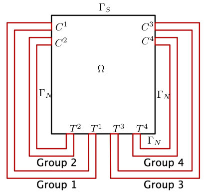 Figure 1
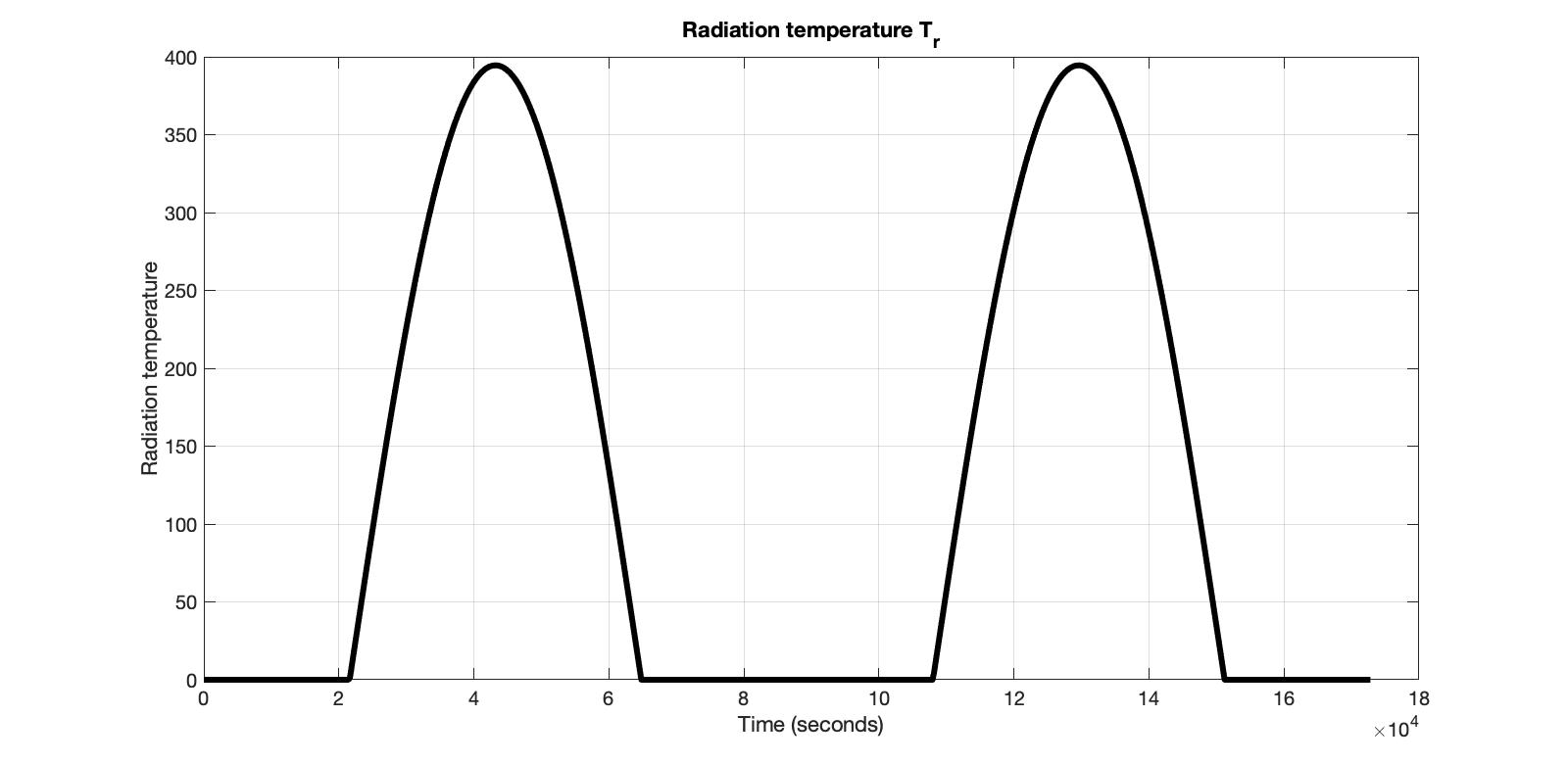 Figure 2
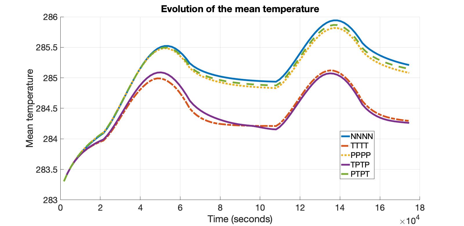 Figure 3
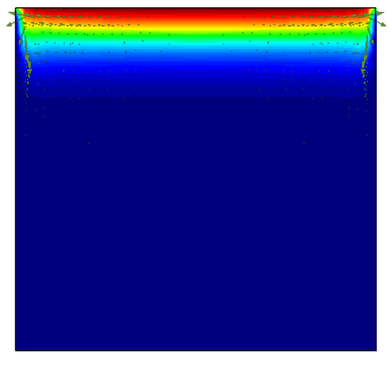 Figure 4
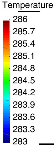 Figure 5
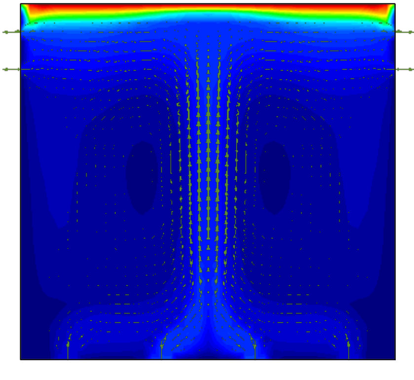 Figure 6
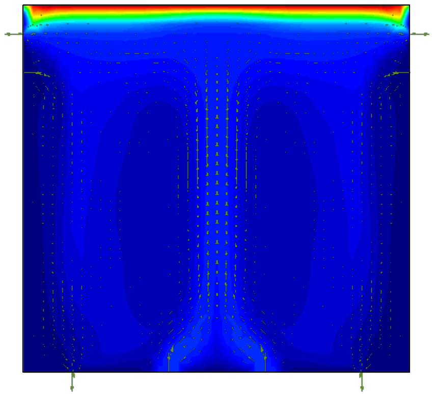 Figure 7
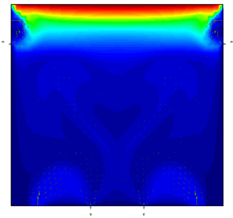 Figure 8
| Parameters | Values | Units |
|---|---|---|
| , | ||
| K | ||
| K | ||
| K | ||
Peer Reviews
No public reviews on file for this paper yet. If you reviewed it on a platform where reviews are public (OpenReview, ICLR, NeurIPS, ICML), you can paste yours below so the community can read it here.
Videos
No videos yet. Explain this paper in a talk, walkthrough, or lecture? Add one.
Mathematical analysis and numerical resolution of a
heat transfer problem arising in water recirculation
Francisco J. Fernández
Lino J. Alvarez-Vázquez Corresponding author. Tel: +34 986 812166. Fax: +34 986 812116. [email protected]
Aurea Martínez
Universidade de Santiago de Compostela, Instituto de Matemáticas, 15782 Santiago, Spain.
Universidade de Vigo, E.I. Telecomunicación, 36310 Vigo, Spain.
Abstract
This work is devoted to the analysis and resolution of a well-posed mathematical model for several processes involved in the artificial circulation of water in a large waterbody. This novel formulation couples the convective heat transfer equation with the modified Navier-Stokes system following a Smagorinsky turbulence model, completed with a suitable set of mixed, nonhomogeneous boundary conditions of diffusive, convective and radiative type. We prove several theoretical results related to existence of solution, and propose a full algorithm for its computation, illustrated with some realistic numerical examples.
keywords:
Radiation heat transfer , Existence , Uniqueness , Numerical resolution
,
,
1 Introduction
Artificial circulation in large waterbodies is a management technique aimed to disrupt stratification of temperature and, consequently, to minimize the development of stagnant zones that may be subject to water quality problems (for instance, low levels of dissolved oxygen or high concentrations of phytoplankton). For its operation, a set of flow pumps take water from the upper layers by means of collectors and inject it into the bottom layers, setting up a recirculation pattern that prevents stratification by means of a forced mixing of water. One of the main problems of the temperature stratification is related to algal blooms produced in the upper layers due to high temperature and solar radiation. However, if we circulate water from the bottom layers (where the temperature is lower) to the upper layers, we can mitigate this negative effect. Further details and remarks on several issues related to the optimal design and control of water artificial circulation techniques have been analyzed by the authors in their recent work [19].
Convective heat transfer has been the subject of an intensive mathematical research in last five decades (ranging, for instance, from the pioneering works on the Boussinesq system of Joseph [15] in the 1960s to the present). Among the recent contributions we must mention, for instance, some papers devoted to study related problems in the steady case [4, 16], the analysis a time-dependant case, but not including convective phenomena, [20], and some numerical approaches [3, 18]. Nevertheless, after an exhaustive search we have not been able to find in the mathematical literature the analysis of the particular problem arising in the setting of our water recirculation model: a coupled problem linking a heat equation with mixed nonlinear boundary conditions to a modified Navier-Stokes equation following the Smagorinsky model of turbulence. Thus, the present work deals with the mathematical analysis and the numerical resolution of this heat transfer problem with specific boundary conditions related to water artificial circulation in a body of water (for instance, a lake or a reservoir). The main difficulties in the study of this problem lie in the nonlinear boundary condition related to the solar irradiation on the surface, the relations between the water temperature in the collectors and the injectors, and the coupling between water temperature and water velocity due to convective effects. We use the Smagorinsky model of turbulence instead of other approaches, like the celebrated system, due to the fact that the modified Navier-Stokes equations following the Smagorinsky model of turbulence present very interesting properties from a mathematical viewpoint, in particular the uniqueness of solution and its additional regularity.
The organization of this paper is as follows: First we introduce a well-posed formulation of the physical problem and present a rigorous definition of a solution for the problem. In the central part of the paper we prove the existence of this solution, and in the final part we propose a numerical algorithm for its resolution, showing several computational tests for a realistic example. At the end of the paper we include an appendix with several results for a general heat equation with an advective term and mixed boundary conditions of diffusive, convective and radiative type. These results, as far as we know, are new since we use techniques that will allow us to treat the low regularity of the time derivative of the solution. This lack of regularity represents, together with the nonlinearity of the boundary conditions, the main difficulty.
2 Mathematical formulation of the problem
In this section we present in detail the three-dimensional mathematical model under study. So, we consider a convex domain (representing the waterbody) whose boundary surface can be split into four smooth enough, disjoint sections: , , and , in such a way that . Subset represents the part of the boundary in contact with air, is the part of the boundary where the collectors are located, is the part of the boundary where the injectors are located, and stands for the rest of the boundary. We will suppose that each collector is linked to an injector by means of a pumped pipeline, and we also assume that there exist collector/injector pairs . Therefore, , and . In Fig. 1 we can see a schematic geometrical configuration of a rectangular domain for a particular case of collector/injector pairs.
As above commented, we suppose the boundary regular enough to assure the existence of elements , , satisfying the following assumptions (corresponding to suitable regularizations of the indicator functions of and , respectively):
- •
, a.e. ,
- •
, a.e. , and ,
- •
, a.e. , and ,
where represents the area measure of any set .
We denote by (measured in K) the solution of the following convection-diffusion partial differential equation with nonhomogeneous, nonlinear, mixed boundary conditions:
[TABLE]
where Dirichlet boundary condition is given by expression:
[TABLE]
with, for each ,
[TABLE]
representing the mean temperature of water in the collector , and with the weight function defined by:
[TABLE]
for the positive constant satisfying the unitary condition:
[TABLE]
In other words, we are assuming that the mean temperature of water at each injector is a weighted average in time of the mean temperatures of water at its corresponding collector . In order to obtain the mean temperature at each injector, we convolute the mean temperature at the collector with a smooth function with support in . In this way, we have that the temperature in the injector only depends on the mean temperature in the collector in the time interval . Parameter represents, in a certain sense, the technical characteristics of the pipeline that define the stay time of water in the pipe. We also suppose that there is not heat transfer thought the walls of the pipelines (that is, they are isolated).
Moreover,
- •
is the length of the time interval.
- •
is the unit outward normal vector to the boundary .
- •
is the thermal diffusivity of the fluid: , where is the thermal conductivity, is the density, and is the specific heat capacity of water.
- •
, for , are the coefficients related to convective heat transfer through the boundaries and , obtained from the relation , where are the convective heat transfer coefficients on each surface. These coefficients are relevant in the convective heat transfer flux through the frontiers and , , .
- •
is the coefficient related to radiative heat transfer through the boundary , given by , where is the Stefan-Boltzmann constant and is the emissivity. This coefficient is fundamental in the radiative flux through the frontier (see, for instance, the classical reference [5] for a complete description of this type of boundary conditions).
- •
is the initial temperature.
- •
are the temperatures related to convection heat transfer on the surfaces and .
- •
is the radiation temperature on the surface , derived from expression , where is the albedo, denotes the net incident shortwave radiation on the surface , and denotes the downwelling longwave radiation.
Finally, is the water velocity, solution of a modified Navier-Stokes equations following a Smagorinsky model of turbulence:
[TABLE]
where is the gravity acceleration, is the thermic expansion coefficient. We must remark here that we are assuming the thermodynamic process to be close to an initial equilibrium state that we denote with the zero subscript, so , where is the isothermal compressibility coefficient. The details of this approach (known as the Boussinesq model for natural convection) can be consulted, for instance, in Section 10.7 of [6]. Finally, is the initial velocity, and boundary field is the element given by:
[TABLE]
with, for each , , representing the volumetric flow rate by pump at each time (, , and ). The turbulence term is given by:
[TABLE]
where is a potential function (for instance, in the particular case of the classical Navier-Stokes equations, , with the kinematic viscosity of the water, and, consequently, ). However, in our case, the Smagorinsky model, the potential function is defined as [17]:
[TABLE]
where is the turbulent viscosity. So, for the Smagorinsky case,
[TABLE]
with .
System (6) has been recently studied by the authors in [9], where it is demonstrated the existence and the uniqueness of solution for a recirculation model based in the modified Navier-Stokes equations. In the present work we will use some of the results shown in [9] in order to prove the existence of solution for the coupled problem (1) and (6). The main difficulties of this work relies in the coupling of a heat equation with nonlinear boundary value terms and the modified Navier-Stokes system. The nonlinear terms do not allow us to work with regular solutions for the heat equation, which forces us to use more sophisticated techniques in order to demonstrate existence and uniqueness of solution.
3 The concept of solution
We start this section defining the functional spaces used in the definition of solution for the system (1) and (6). So, for the water temperature we consider:
[TABLE]
and we define the following norm associated to above space :
[TABLE]
We have that is a reflexive separable Banach space (cf. Lemma 3.1 of [8]) and is an evolution triple. For the water velocity we consider:
[TABLE]
In order to define an appropriate space for the solution of problems (1) and (6), we consider, for a Banach space and a locally convex space such that , the following Sobolev-Bochner space (cf. Chapter 7 of [21]), for :
[TABLE]
where denotes the derivative of in the sense of distributions. It is well known that, if both and are Banach spaces, then is also a Banach space endowed with the norm .
Then, we define the following spaces that will be used in the mathematical analysis of system (1):
[TABLE]
and, for the system (6), we define
[TABLE]
Hypothesis 1
We will assume the following hypotheses for coefficients and data of the problem:
- (a)
** 2. (b)
** 3. (c)
** 4. (d)
** 5. (e)
** 6. (f)
* with , *
Remark 2
In order to define in a rigorous way the concept of solution, we will need to extend Dirichlet conditions of and to the whole domain .
So, for water velocity , thanks to Lemma 2 of [9], for each , there exists an element such that , with defined by (7). Besides, by Lemma 3 of [9], and, then, we can use this element to reformulate the original problem for as an homogeneous Dirichlet boundary condition one.
For water temperature we can proceed in an analogous way and prove that there exists an extension that allows us to reformulate the problem for as one with homogeneous boundary conditions.
Lemma 3
We have that the following operator is compact
[TABLE]
where:
[TABLE]
with , for , defined by:
[TABLE]
and the right inverse of the classical trace operator (that is, .)
We also have that there exists a constant , that depends continuously on the space-time configuration of our computational domain and , such that:
[TABLE]
{@proof}
[Proof.] Let be a bounded sequence in . Then, taking subsequences if necessary, we have that weakly in . We also have that weakly in and, if we denote by
[TABLE]
we obtain that pointwise a.e. , . Thus, the sequence is bounded by a function in , so we have the strong convergence in . We can repeat the same argument with the time derivative of , obtaining that strongly in , thus strongly in . Finally, by the properties of the operator we have that
[TABLE]
So, thanks to the regularity of function , it is clear that , and
[TABLE]
In the other hand,
[TABLE]
Thereby, we have the following inequality:
[TABLE]
where is a positive constant than depends continuously on the spatial-time configuration of our computational domain and on the initial temperature. Moreover, it is worthwhile remarking here that we can make this constant as small as we want by considering data appropriately.
Finally, the following technical lemma will be necessary in order to guaranty that the sum of an element of plus an element of makes sense.
Lemma 4
We have that the following inclusion is compact:
[TABLE]
Now, we define the concept of solution for coupled system (1) and (6) in terms of homogeneous Dirichlet systems, so we establish the following notations:
- •
, with the extension obtained from Lemma 3, where:
[TABLE]
- •
, with the extension of the trace given in Lemma 2 of [9].
Thus, using above notations, we can reformulate the state system (1) and (6) in the following way:
[TABLE]
[TABLE]
It is worthwhile remarking here that above system shows homogeneous Dirichlet boundary conditions and, consequently, we will be able to define the concept of solution of the original state systems (1) and (6) in terms of the modified state systems (27) and (28). It should be also noted that, in the case of equation (1), the coupling terms in the Dirichlet boundary conditions are now transferred to the partial differential equation in system (27).
Definition 5
A pair is said to be a solution of problem (1) and (6) if there exist elements such that:
, with the reconstruction of the trace given in Lemma 2 of **[9]**, and , with the extension obtained in Lemma 3, where:
[TABLE] 2. 2.
, and , a.e. . 3. 3.
* verifies the following variational formulation:*
[TABLE]
[TABLE]
where
[TABLE]
4 Existence of solution
We will prove now that, under certain hypotheses over coefficients and data, there exists a unique solution for the system (1) and (6) in the sense of Definition 5. The procedure used here for demonstrating the existence of solution is based in the Schauder fixed point Theorem (cf. section 9.5 of [7]) and is similar to one employed by the authors, for instance, in [10]. The main difficulties in the present case lie in the coupling of the Dirichlet conditions for the water temperature, and in the nonlinear radiation terms. To overcome these difficulties we will need to define a compact extension for the nonhomogeneous Dirichlet conditions and to prove novel results for the heat equation with radiation boundary conditions (see Appendix A).
So, we consider the following operator:
[TABLE]
where:
- •
is such that is the solution of the following problem:
[TABLE]
with the extension obtained from the Lemma 2 of [9].
- •
is such that is the solution of:
[TABLE]
with defined as in Lemma 3.
- •
is such that:
[TABLE]
The following technical results are necessary to prove that the operator defined in (33) is well defined. The first one corresponds to the existence of solution for problem (34), and the second one is related to the existence of solution for problem (35).
Theorem 6
Within the framework stablished in Hypothesis 1, given elements and , there exists an element such that is the unique solution of problem (34) in the following sense:
[TABLE]
with , a.e. , where:
[TABLE]
Besides, we have the following estimates:
[TABLE]
[TABLE]
where and are positive constants that depend continuously with respect to the space-time configuration of our computational domain, , and .
{@proof}
[Proof.] It is a direct consequence of Theorem 8 in [9]. In this theorem the authors prove the wellposedness (existence, uniqueness and regularity of solution) for a modified Navier-Stokes system with non-homogeneous Dirichlet boundary conditions, by building a continuous extension of the Dirichlet condition and a Galerking approximation of the corresponding problem with homogeneous boundary conditions.
Theorem 7
Within the framework stablished in Hypothesis 1, given elements and , there exits an element such that is the unique solution of problem (35) in the following sense:
[TABLE]
with , a.e. .
Besides, we have the following estimates:
[TABLE]
[TABLE]
where and are positive constants that depend continuously with respect to the space-time configuration of our computational domain, , , and .
{@proof}
[Proof.] It is a straightforward consequence of Theorem 14 that we will prove in Appendix A. In our case, we have to choose there , and .
Lemma 8
The operator defined in (33) is well defined and compact.
{@proof}
[Proof.] Thanks to above Theorems 6 and 7, it is straightforward that the operator is well defined. Let us check now its compactness.
So, given a bounded sequence , we have, using estimates (39) and (40), that the corresponding sequence of solutions for the problem (37) is bounded in . Then, we have, taking subsequences if necessary, that:
- •
in ,
- •
in ,
- •
strongly in , for all , and ,
- •
weakly in ,
- •
weakly in ,
- •
weakly- in ,
- •
weakly in ,
where is the solution of (37) associated to . The last convergence is a consequence of the monotony of operator (see [9] for more details)
[TABLE]
where, for any ,
[TABLE]
Now, using the results proved in Lemma 3, we have that the corresponding sequence converges to strongly in , and, consequently,
- •
in ,
- •
in ,
- •
in ,
- •
in .
Finally, thanks to estimates (42) and (43), the corresponding sequence is bounded. Thus, taking subsequences if necessary, we have thanks to a straightforward adaptation of Lemma 19 in Appendix A, that
- •
in ,
- •
in ,
- •
in ,
- •
in ,
- •
in .
Using the same techniques that we present in Appendix A for the demonstration of Theorem 14, we can pass to the limit in the variational formulation of and prove that is the solution of (7) associated to and . Thus, we have that
- •
in ,
- •
in ,
and, consequently, in , which concludes the proof.
Theorem 9
Given positive constants and , there exist coefficients and data small enough such that the operator defined in (33) has a fixed point in the space . Moreover, the corresponding is a solution for the system (1) and (6) in the sense of Definition 5.
{@proof}
[Proof.] The existence is a direct consequence of the Schauder fixed point Theorem. Given an element , we have, thanks to (20), (39), (40), (42) and (43), the following estimates for :
[TABLE]
where , , are positive constants that depend continuously on the coefficients and data. If we take the first inequality to the second and third ones, we obtain that:
[TABLE]
So, if we suppose that and , we have that
[TABLE]
Thus, we are led to solve the following inequality:
[TABLE]
However, it is obvious that, given and , we can consider small enough data , , , , and , such that
[TABLE]
Then, choosing suitable coefficients and data that verify (48)-(50), we have that maps elements of the set into itself. Thus, thanks to Schauder fixed point Theorem, there exists a fixed point of operator , such that the corresponding is a solution of the coupled system (1) and (6) in the sense of Definition 5.
5 Numerical resolution
Once proved in above section that the coupled system (1) and (6) admits a solution, we will introduce here a full numerical algorithm in order to compute it, and show several computational test for a realistic example.
We must recall here that our main aim is related to understanding which is the best strategy for reducing the water temperature in the upper layers. In order to achieve this objective, and for the sake of completeness, we will consider an algorithm able to deal with more general states than those we have presented in previous mathematical analysis of the problem. In particular, in the numerical resolution proposed here we will also take into account the possibility that takes non-positive values. To be exact, if we will say that the pump is turbinating (water enters by the collector and is turbinated by the corresponding pipeline to the injector ), and if we will say that the pump is pumping (water enters by injector and is pumped to the collector ). As it is evident, the situation corresponds to the case in which the pump is off. In addition, we will also suppose that the parameter used in the definition (2) tends to cero, that is, the mean temperature in the injectors is equal to the mean temperature in the collectors. It is essential emphasizing here that it is also possible to perform a similar mathematical analysis for the general case (with the obvious embarrassing notations), under the only assumption of the existence of a partition of the time interval verifying that the groups do not change their state within any element of the partition (as can be seen in following section devoted to the numerical examples).
5.1 Space-time discretization
For the discretization of the problem, let us consider a regular partition of the time interval such that , , and a family of meshes for the domain with characteristic size . Associated to this family of meshes, we also consider three compatible finite element spaces , and corresponding, respectively, to the water temperature, velocity and the pressure of water. From the computational viewpoint, for the generation of the mesh associated to the domain and for the numerical resolution of the system, we propose the use of FreeFem++ [14]. Finally, we have employed an Uzawa algorithm [12] for computing the solution of the Stokes problems that appears after the discretization, and a fixed point algorithm for solving the nonlinearities.
So, we consider the following space-time discretization for system (1) and (6):
Dirichlet condition for the water velocity: We consider the following approximation for a function ,
[TABLE]
where, for all , is such that , and , . It is well known that the linear closure of the functions of the basis is a vector subspace of , so if we suppose that , , we can consider the following coordinate vector in the basis of the corresponding subspace of :
[TABLE]
with , , , with a technical bound related to mechanical characteristics of pumps. 2. 2.
Coupling of temperature in collectors and injectors: We denote by the water temperature at time step . Then, we can consider the following approximation in the case of , , , for (3) by functions , , :
[TABLE]
Moreover, if we assume the value in the definition (4) of function we have that the support of is contained in , for all , and then:
[TABLE]
Finally, we approximate each element by the indicator function of the injector , , and each element by the indicator function of the collector , . Thus, the temperature in each injector at time step is the mean temperature in the corresponding collector at time step . The previous approximation is still valid in the general case with obvious modifications. For instance, if we suppose that , , , then, we consider the Dirichlet condition in the collectors:
[TABLE] 3. 3.
Water temperature: Given , is the solution of:
[TABLE]
where the discrete characteristic .
Then, for each , , with
[TABLE]
for all , is the solution of:
[TABLE]
where the discrete characteristic , for , and where the functional space is given by:
[TABLE]
with denoting the sign function:
[TABLE]
For instance, in the case of for all , , then , so
[TABLE]
That is, we are considering the Dirichlet condition on the injectors. In the oposite case, for all , , we have that
[TABLE]
and we are considering the Dirichlet condition on the collectors. In the general case, we can have alternating Dirichlet conditions on the collectors and injectors, so the definition for the space , , given in (58) covers all the possibilities. 4. 4.
Water velocity and pressure: Given , for each , the pair velocity/pressure , with:
[TABLE]
is the solution of:
[TABLE]
where the functional space .
Remark 10
It is worthwhile noting here that in above scheme we have to compute one additional time step for the water temperature. This shift is motivated by the dependence diagram shown in Fig. 2. We observe that, due to the time discretization proposed here, the Dirichlet boundary condition for the hydrodynamic model begins to have influence from the second step of time for the water temperature. In the first time step , water circulation does not affect the water temperature, so for this first time step we consider . However, for , we impose at each of the collector/injector pairs one of the boundary conditions (54), (55) or (56), depending on the sign of the Dirichlet condition in previous time step.
5.2 Numerical results
This final subsection is devoted to present some numerical results that we have obtained using realistic coefficients and data. Nevertheless, for the sake of clarity and comprehensibility, we will show results for a simplified 2D domain. For this purpose, we have considered a rectangular domain (measured in meters), corresponding a reservoir, in which we have distributed collector/injector pairs with a symmetrical configuration similar to that shown in Fig. 1. For the time discretization we have chosen a time step of seconds with time steps (which represents a time period of 2 days), and for the space discretization we have used a regular mesh formed by triangles of characteristic size meters (corresponding to vertices). Finally, the finite element spaces employed for space discretizations have been the Taylor-Hood element for the hydrodynamic model, and the Lagrange element for the water temperature. In Fig. 3 we can observe the evolution of the radiation temperature:
[TABLE]
along the whole period of 2 days ( seconds), considering , , (typical values in mediterranean countries during the summer) and multiplied by a sinusoidal function in order to simulate the effects of day and night. The parameters used for the numerical resolution of the coupled system can be seen in Table 1.
In order to analyze the influence of water artificial circulation in the thermal behavior of top meters from water upper layer we have solved the problem in five different scenarios:
NNNN: In this configuration we take , for all and (reference configuration with all the groups off). 2. 2.
TTTT: In this configuration we take , for all and (all the groups are turbinating). 3. 3.
PPPP: In this configuration we take , for all and (all the groups are pumping). 4. 4.
TPTP: In this configuration we take and , for all and (groups and are turbinating, and groups and are pumping). 5. 5.
PTPT: In this configuration we take and , for all and the groups and are turbinating).
In Fig. 4 we present the evolution of the mean temperature in the top meters upper layer along the whole time interval corresponding to two days. We can clearly distinguish here that the best configurations correspond, in a very evident manner, to the second scenario (TTTT) and to the fourth one (TPTP). Moreover, we can notice how third and fifth scenarios (PPPP and PTPT, respectively) do not improve in a significant way the reference configuration (NNNN).
Finally, we show in Fig. 5 water temperatures and velocities at last time step for NNNN and TTTT configurations and, in Fig. 6, the behavior of water at same time step for configurations TPTP and PTPT. (In all of the cases, velocities have been multiplied by an amplifying factor to make their graphic representations more perceptible). As we can easily notice, the best strategies correspond to evacuating the excess of temperature in the upper layers to the bottom layers instead of refrigerating the upper layers with cold water from the bottom ones.
Although we only present here one realistic example of application of our approach to understand the behaviour of water velocity and temperature in the upper section of the domain, we have developed many other numerical experiences for different choices of parameters and data (that will not be presented here for the sake of conciseness). However, from these computational tests we can derive two important consequences: For the modified Navier-Stokes equations, the second member -corresponding to the thermic term- shows less influence in the numerical resuls than the Smagorinsky turbulence term. For the convective heat equation, the radiation term in the nonlinear boundary condition affects in a significative way the final results. Finally, for a better resolution of the numerical examples, it would be possible to use, instead of an uniform mesh like the one employed in previous example, a finer mesh in the neighbourhoods of collectors and injectors. Nevertheless, this approach would mean a significant increase in the computational time, already quite high in the current case (especially in the part referring to the resolution of the hydrodynamic problem).
Acknowledgments
The authors thank the funding from project MTM2015-65570-P of MINECO/ FEDER (Spain).
Appendix A A radiation heat transfer problem with nonhomogeneous mixed boundary conditions
In this appendix we mathematically analyze a heat equation with an advective term and mixed boundary conditions of diffusive, convective and radiative type. The essential difficulty for demonstrating the existence and uniqueness of solution lies, in one hand, in the presence of nonlinear boundary conditions of radiative type and, in the other hand, the lack of regularity of the time derivative of the solutions. This lack of regularity does not allow us to take the solution itself as a test function in the variational formulation, and we are led to use more refined techniques (similar to those employed, for instance, in [1]).
So, we suppose that we have a convex domain , whose boundary can be split into three disjoint, smooth enough parts: , and , with . We denote by the solution of the following initial-boundary value problem:
[TABLE]
where is the thermal diffusivity, , for , are the coefficients related to convective heat transfer through the boundaries and , and is the coefficient related to radiative heat transfer through the boundary , is the initial temperature, is Dirichlet temperature on , is the radiation temperature on , and are the temperatures related to convection heat transfer in surfaces and .
Remark 11
In this work we will suppose that , and are nonempty, but all the results can be easily extended to the case where and/or are empty sets. The only drawback is when because in this case we cannot use Poincare type inequalities, and we should apply another type of techniques for obtaining energy estimates in the Galerkin approximation. A related problem with was studied, for instance, in [20].
We consider the following spaces
[TABLE]
and
[TABLE]
Hypothesis 12
We will assume the following hypotheses for the coefficients and data:
. 2. 2.
. 3. 3.
. 4. 4.
. 5. 5.
. 6. 6.
. 7. 7.
, a.e. , with and , where .
Definition 13
Within the framework established in Hypothesis 12, we say that an element is a solution of the system (64) if there exists such that:
- •
, with , where is the right inverse of trace operator .
- •
, a.e. .
- •
* is the solution of the following variational formulation:*
[TABLE]
where some of previous integrals must be understood as duality pairs, and
[TABLE]
We have the following result that we will prove in the following subsections:
Theorem 14
Within the framework established in Hypothesis 12, there exists a unique solution of equation (67) in the sense of Definition 13. Moreover, there exists a constant , such that this solution satisfies the following inequalities:
[TABLE]
[TABLE]
In order to better understand the proof of the previous result, we will divide it in five parts: in the first part we will prove some technical results related to the space where we look for the solution. In the second part we will obtain the Galerkin approximation of problem (64). In the third part we will analyze the differential equation obtained from the Galerkin discretization. In the fourth part we will derive the convergence of the Galerkin approximation in a suitable space. Finally, in fifth part we will prove Theorem 14.
A.1 Part 1: Some technical results
We have the following lemma that we will use in following subsections:
Lemma 15
Let a Banach space such that . The following inclusion is compact:
[TABLE]
{@proof}
[Proof.] The proof is a direct consequence of Aubin and Lions Lemma (see, for instance, Lemma 7.7 of [21]), the compactness of in and the fact that is is an interpolant between and . Indeed, given a bounded sequence in we have that there exists a subsequence, that we will still denote in the same way, such that in and in . We realize that in because:
[TABLE]
when .
Remark 16
We have that (in fact, it is well known that if and continuously, then continuously), and that . Then, the sum makes sense in the space . Moreover, .
We can also consider as a Dirichlet condition the restriction to of one element of the space , with . In this case, we can obtain an extension in the space (cf. Theorem 3.2 of [11]) and, if we want to ensure that , we can take, for instance, .
A.2 Part 2: Galerkin approximation
In this part we will construct a sequence of approximations that will converge to a solution of problem (64). So, let be a dense subset of independent vectors of , such that , , which we can assume orthonormal in . We also assume that the projection
[TABLE]
is selfadjoint and , , where is a Banach space, as given in Lemma 15. Then, for , we denote by:
[TABLE]
where the coefficients , , are such that is the solution of the following differential equation:
[TABLE]
which can be rewritten in the following standard formulation:
[TABLE]
where:
[TABLE]
[TABLE]
[TABLE]
[TABLE]
[TABLE]
[TABLE]
where , and is the projection of onto .
Thus, we say than an element is a solution of system (75) if it satisfies the ordinary differential equation problem (76). We must recall here that , , and that, if is a solution of problem (75), then .
Lemma 17
Within the framework established in Hypothesis 12, there exits a constant independent of such that:
[TABLE]
[TABLE]
{@proof}
[Proof.] Multiplying (75) by , summing in and adding to both sides the term
[TABLE]
we have:
[TABLE]
As a consequence of the continuity of trace operator and of the inequalities of Young and Poincare, we obtain:
[TABLE]
where , , are arbitrary strictly positive numbers, and , , are constants that may depend on the trace operator and Young and Poincare’s inequalities. If we take , , such that and , then (renaming the constants if necessary):
[TABLE]
Adding to both sides , using the inequality (for ), and taking :
[TABLE]
Finally, integrating over the time interval (renaming again the constants):
[TABLE]
where we have used that , . Finally, applying Gronwall’s Lemma, we obtain that there exists a positive constant independent of such that (83) is satisfied.
For obtaining (84) it is sufficient to apply Holder inequality and bear in mind the fact that the projection operator onto is bounded independently of :
[TABLE]
A.3 Part 3: Existence of solution for the Galerkin approximation
Now we will demonstrate that there exists, for each , a unique absolutely continuous solution of equation (75).
Lemma 18
Within the framework established in Hypothesis 12, there exists a unique absolutely continuous solution defined on the whole time interval of Cauchy problem (76).
{@proof}
[Proof.] To state this lemma we can apply the Caratheodory theorem for ordinary differential equations (cf., for example, Theorem 5.2 of [13]). Indeed, is continuous for any , and for any . Then, given an open ball in , if we prove that there exist two functions such that:
[TABLE]
we can conclude that problem (76) has a unique absolutely continuous solution, which can be extended to the boundary of . It is worthwhile mentioning here that, if
[TABLE]
then the solution cannot reach the boundary of because of the a priori estimate (83) and the fact that . The first of the Caratheodory conditions (90) can be obtained by applying Holder inequality (in fact, we obtain that ). In the other hand, for the second Caratheodory condition, we can use the following inequality (straightforward consequence of the mean value Theorem):
[TABLE]
for and . So, we obtain the following inequality:
[TABLE]
Therefore, we can conclude the existence of a function (in fact, such that the second of the Caratheodory conditions (90) is achieved.
A.4 Part 4: Convergence of the Galerkin approximation
In previous subsections we have seen that there exists a bounded sequence of solutions of problem (76). In this subsection we will pass to the limit and obtain a solution of equation (67).
Lemma 19
There exists a subsequence of , still denoted in the same way, such that:
* in ,* 2. 2.
* in ,* 3. 3.
* in ,* 4. 4.
* in ,* 5. 5.
* in **.*
{@proof}
[Proof.] Thanks to the boundedness in of the sequence , we obtain the first two convergences. The third and fourth limits are a direct consequence of Aubin, and Lions Lemma (cf. Lemma 7.7 of [21]) and the compactness of , respectively, in and , . Finally, the fifth convergence is a consequence of Lemma 15.
Lemma 20
If is a bounded sequence in , then there exists a subsequence of , still denoted in the same way, such that, for all :
[TABLE]
{@proof}
[Proof.] Using the same technique that we have employed in the proof of Lemma 18, from the strong convergence of to in we have:
[TABLE]
A.5 Part 5: Proof of the main result of the Appendix
Now, we can demonstrate the Theorem 14:
{@proof}
[Proof.] We will divide the proof into three parts, in the first part we will pass to the limit in the Galerkin approximation in order to obtain a solution for the system (67), in the second part, we will derive the estimates (69) and (70) and, finally, in the third part we will prove the uniqueness of solution.
First, for a fixed index , if we multiply (75) by a scalar function continuously differentiable on , such that , integrate with respect to , and integrate by parts, we have, :
[TABLE]
The passage to the limit for in the integrals of the left-hand side is due to the Lemmas 19 and 20. We observe also that in . Hence, we find in the limit:
[TABLE]
for each which is a finite lineal combination of elements . Since each term of above expression depends linearly and continuously on , for the norm of , previous equality remains still valid, by continuity, for each . Now, writing in particular (95) for , we obtain the variational formulation (67). Finally, we can prove that multiplying (67) by the same as before, integrating by parts with respect to , and comparing with (95).
Then, multiplying inequality (89) by , with , , and integrating in we have:
[TABLE]
from which, taking into account that the norm of a reflexive Banach space is weakly lower semicontinuous, we can pass to the inferior limit thanks to convergences of Lemma 19:
[TABLE]
Thus, we obtain the following energy inequality for a.e. :
[TABLE]
Finally, (69) can be derived from above expression thanks to the Gronwall’s Lemma, and estimate (70) is a direct consequence of Holder inequality.
Now, we will prove the uniqueness of solution. Let us assume the existence of two solutions and for problem (67), and define . We have that , , a.e. , and that satisfies the following variational formulation:
[TABLE]
From a direct computation, we observe that , where , and , defined by:
[TABLE]
, \ \ \beta=-b_{2}^{R}\big{[}|{\xi_{1}}_{|_{\Gamma_{R}}}+{\zeta_{D}}_{|_{\Gamma_{R}}}|^{3}({\xi_{1}}_{|_{\Gamma_{R}}}+{\zeta_{D}}_{|_{\Gamma_{R}}})-|{\xi_{2}}_{|_{\Gamma_{R}}}+{\zeta_{D}}_{|_{\Gamma_{R}}}|^{3}({\xi_{2}}_{|_{\Gamma_{R}}}+{\zeta_{D}}_{|_{\Gamma_{R}}})\big{]}, and .
Now, for each , we define the following function:
[TABLE]
and its primitive,
[TABLE]
We can extend the results proved in Corollary 9 of [2] to our case (we just need to add the term in in the proof of Lemma 6 of [2] and then we can use this result to prove Corollary 9) and then, we have:
[TABLE]
By a direct evaluation of previous expression, we have:
[TABLE]
a.e. . Moreover, it is obvious that:
[TABLE]
for and , a.e. . Thus, we can deduce that:
[TABLE]
Finally, from the definition (101) of it is straightforward that , , and then:
[TABLE]
with denoting the volume of , which implies that , a.e. , and, consequently, .
The reference list from the paper itself. Each links out to its DOI / PubMed record.
- 1[1] L.J. Alvarez-Vázquez, F.J. Fernández, and R. Muñoz-Sola. Mathematical analysis of a three-dimensional eutrophication model. J. Math. Anal. Appl. , 349:135–155, 2009.
- 2[2] L.J. Alvarez-Vázquez, F.J. Fernández, and R. Muñoz-Sola. Analysis of a multistate control problem related to food technology. J. Diff. Equations , 245:130–153, 2008.
- 3[3] A. Bahlaoui, A. Raji, and M. Hasnaoui. Multiple Steady State Solutions Resulting From Coupling Between Mixed Convection And Radiation In An Inclined Channel. Heat Mass Transfer , 41:899–908, 2005.
- 4[4] M. Benes and P. Kucera. On the Navier-Stokes flows for heat-conducting fluids with mixed boundary conditions. J. Math. Anal. Appl. , 389:769–780, 2012.
- 5[5] T.L. Bergman, A.S. Lavine, F.P. Incropera, and D.P. De Witt. Fundamentals of Heat and Mass Transfer . John Wiley & Sons, New York, 2011.
- 6[6] A. Bermúdez de Castro. Continuum Thermomechanics . Birkhauser, Basel, 2005.
- 7[7] J.B. Conway. A course in functional analysis . Springer-Verlag, New York, 1990.
- 8[8] M.C. Delfour, G. Payre, and J.P. Zolesio. Approximation of nonlinear problems associated with radiating bodies in space. SIAM J. Numer. Anal. , 24:1077–1094, 1987.