Flat trace statistics of the transfer operator of a random partially expanding map
Luc Gossart

TL;DR
This paper studies the statistical behavior of the transfer operator associated with a randomly perturbed expanding map on the circle, revealing that its flat traces follow a normal distribution in the semiclassical limit up to a logarithmic Ehrenfest time.
Contribution
It demonstrates that the flat traces of the transfer operator exhibit Gaussian fluctuations in the semiclassical limit for a class of random partially expanding maps.
Findings
Flat traces behave as normal distributions in the semiclassical limit.
Behavior holds up to the Ehrenfest time proportional to log of frequency.
Results extend understanding of transfer operators in random dynamical systems.
Abstract
We consider the skew-product of an expanding map on the circle with an almost surely random perturbation of a deterministic function : \[F :\left\{\begin{array}{rcl} \mathbb T \times \mathbb R & \longrightarrow & \mathbb T \times \mathbb R\\ (x,y)& \longmapsto & (E(x), y+\tau(x))\\ \end{array} \right.\] The associated transfer operator can be decomposed with respect to frequency in the variable into a family of operators acting on functions on the circle: \[\mathcal L_\xi :\left\{\begin{array}{rcl} \mathcal C^k(\mathbb T) & \longrightarrow & \mathcal C^k(\mathbb T)\\ u & \longmapsto & e^{i\xi\tau}u\circ E \\ \end{array} \right.\] We show that the flat traces of behave as normal distributions in the semiclassical limit $n,…
Click any figure to enlarge with its caption.
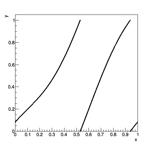 Figure 1
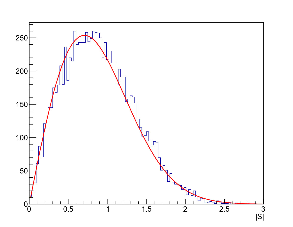 Figure 2
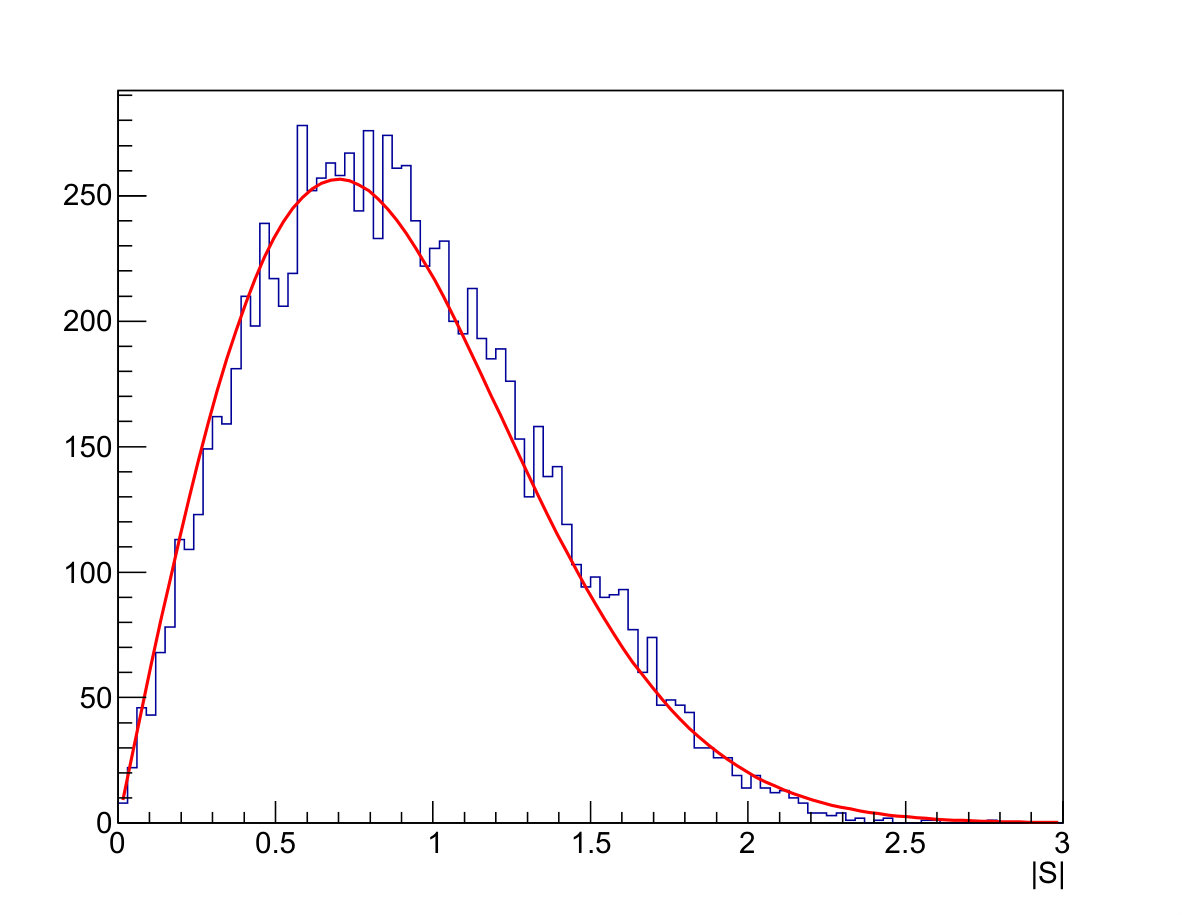 Figure 3
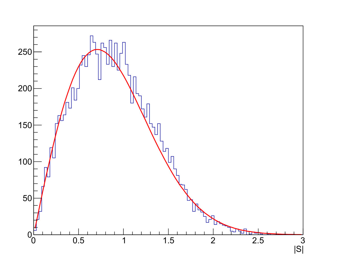 Figure 4
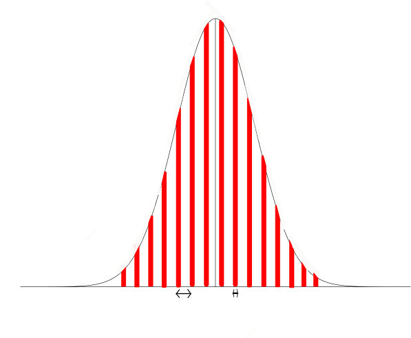 Figure 5
Peer Reviews
No public reviews on file for this paper yet. If you reviewed it on a platform where reviews are public (OpenReview, ICLR, NeurIPS, ICML), you can paste yours below so the community can read it here.
Videos
No videos yet. Explain this paper in a talk, walkthrough, or lecture? Add one.
Taxonomy
TopicsGeometry and complex manifolds · Mathematical Dynamics and Fractals · Stochastic processes and financial applications
Flat traces for a random partially expanding map
Luc Gossart
Institut Fourier, 100, rue des maths BP74 38402 Saint-Martin d’Heres France1112010 Mathematics Subject Classification. 37D30 Partially hyperbolic systems and dominated splittings, 37E10 Maps of the circle, 60F05 Central limit and other weak theorems, 37C30 Zeta functions, (Ruelle-Frobenius) transfer operators, and other functional analytic techniques in dynamical systems.
Abstract.
We consider the skew-product of an expanding map on the circle with an almost surely random perturbation of a deterministic function :
[TABLE]
The associated transfer operator can be decomposed with respect to frequency in the variable into a family of operators acting on functions on the circle:
[TABLE]
We show that the flat traces of behave as normal distributions in the semiclassical limit up to the Ehrenfest time .
Acknowledgements
The author thanks Alejandro Rivera for his many pieces of advice regarding probabilities, and Jens Wittsten, Masato Tsujii, Gabriel Rivière and Sébastien Gouëzel for interesting discussions about this work, as well as the anonymous referees for their careful reading and constructive suggestions.
Contents
1. Introduction
This paper focuses on the distribution of the flat traces of iterates of the transfer operator of a simple example of partially expanding map. It is motivated by the Bohigas-Gianonni-Schmidt [BGS84] conjecture in quantum chaos (see below).
In chaotic dynamics, the transfer operator is an object of first importance linked to the asymptotics of the correlations. The collection of poles of its resolvent, called Ruelle-Pollicott spectrum, can be defined as the spectrum of the transfer operator in appropriate Banach spaces (see [Rue76] for analytic expanding maps, [Kit99], [BKL02], [BT07], [BT08], [GL06], [FRS08] for the construction of the spaces for Anosov diffeomorphisms.)
The study of the Ruelle spectrum for Anosov flows is more difficult because of the flow direction that is neither contracting nor expanding. Dolgopyat has shown in particular in [Dol98] the exponential decay of correlations for the geodesic flow on negatively curved surfaces, and Liverani [Liv04] generalized this result to all contact Anosov flows. His method involved the construction of anisotropic Banach spaces in which the generating vector field has a spectral gap, and no longer relies on symbolic dynamics that prevented from using advantage of the smoothness of the flow. Tsujii [Tsu10] constructed appropriate Hilbert spaces for the transfer operator of contact Anosov flows, and gave explicit upper bounds for the essential spectral radii in terms of and the expansion constants of the flow. Butterley and Liverani [BL07] and later Faure and Sjöstrand [FS11] constructed good spaces for Anosov flows, without the contact hypothesis. Weich and Bonthonneau defined in [BW17] Ruelle spectrum for geodesic flow on negatively curved manifolds with a finite number of cusps. Dyatlov and Guillarmou [DG16] handled the case of open hyperbolic systems. A simple example of Anosov flow is the suspension of an Anosov diffeomorphism, or the suspension semi-flow of an expanding map. Pollicott showed exponential decay of correlations in this setting under a weak condition in [Pol85] and Tsujii constructed suitable spaces for the transfer operator and gave an upper bound on its essential spectral radius in [Tsu08].
In this article we study a closely related discrete time model, the skew product of an expanding map of the circle. It is a particular case of compact group extension [Dol02], which are partially hyperbolic maps, with compact leaves in the neutral direction that are isometric to each other. Dolgopyat showed in [Dol02] that the correlation decrease generically rapidly for compact group extensions, and exponentially in the particular case of expanding maps. In our setting of skew-product of an expanding map of the circle, Faure [Fau11] has shown using semi-classical methods an upper bound on the essential spectral radius of the transfer operator under a condition shown to be generic by Nakano Tsujii and Wittsten [NTW16]. De Simoi, Liverani, Poquet and Volk [de2017fast] and de Simoi and Liverani [de2016statistical] [de2018limit] studied fast-slow dynamical systems, that generalize -extensions of circle expanding maps. The roof function, depending on two variables is multiplied by a small amplitude, and the authors obtained results about the statistical properties, for long time and small . Arnoldi, Faure, and Weich [AFW17] and Faure and Weich [FW17] studied the case of some open partially expanding maps, iteration function schemes, for which they found an explicit bound on the essential spectral radius of the transfer operator in a suitable space, and obtained a Weyl law (upper bound on the number of Ruelle resonances outside the essential spectral radius). Naud [Nau16] studied a model close to the one presented in this paper, in the analytic setting, in which the transfer operator is trace-class, and used the trace formula, in the deterministic and random case to obtain a lower bound on the spectral radius of the transfer operator. In the more general framework of random dynamical systems in which the transfer operator changes randomly at each iteration, for the skew product of an expanding map of the circle, Nakano and Wittsten [NW15] showed exponential decay of correlations.
Semiclassical analysis describes the link between quantum dynamics and the associated classical dynamics in a symplectic manifold. The transfer operator happens to be a Fourier integral operator and the semi-classical approach has thus shown to be useful. The famous Bohigas-Giannoni-Schmidt [BGS84] conjecture of quantum chaos states that for quantum systems whose associated classical dynamic is chaotic, the spectrum of the Hamiltonian shows the same statistics as that of a random matrix (GUE, GOE or GSE according to the symmetries of the system)(see also [Gut13] and [GVZJ91]). We are interested analogously in investigating the possible links between the Ruelle-Pollicott spectrum and the spectrum of random matrices/operators. At first we try to get informations about the spectrum using a trace formula. More useful results could follow from the use of a global normal form as obtained by Faure-Weich in [FW17].
1.1. Expanding map
Let us consider a smooth orientation preserving expanding map on the circle , that is, satisfying , of degree , and let us call
[TABLE]
and
[TABLE]
1.2. Transfer operator
Let us fix a function for some . We are interested in the partially expanding dynamical system on defined by
[TABLE]
We introduce the transfer operator
[TABLE]
1.3. Reduction of the transfer operator
Due to the particular form of the map , the Fourier modes in are invariant under : if for some and some ,
[TABLE]
then
[TABLE]
Given and a function , let us consequently consider the transfer operator defined on functions by
[TABLE]
1.4. Spectrum and flat trace
In appropriate spaces, the transfer operator has a discrete spectrum outside a small disk, the eigenvalues are called Ruelle resonances. It is in general not trace-class, but one can define its flat trace (see Appendix C for a more precise discussion about Ruelle resonances, flat trace and their relationship).
Lemma 1.1** (Trace formula, [AB67], [G*+*77]).**
For any function on , the flat trace of is well defined and
[TABLE]
where denotes the Birkhoff sum: For a function and a point we define
[TABLE]
1.5. Gaussian random fields
We define our random functions on the circle by means of their Fourier coefficients. We are only interested in functions. We will denote by (respectively ) the real (respectively complex) centered Gaussian law of variance , with respective densities
[TABLE]
With these conventions, a random variable of law has independent real and imaginary parts of law , and the variance of its modulus is consequently .
Definition 1.2**.**
We will call centered stationary Gaussian random fields on the real random distributions whose Fourier coefficients are independent complex centered Gaussian random variables, with variances growing at most polynomially, such that is a real centered Gaussian variable independent of the . The negative coefficients are necessarily given by
[TABLE]
The Gaussian fields are in general defined as distributions if their Fourier coefficients have variances with polynomial growth and the decay of the variances of the coefficients gives sufficient conditions for the regularity of the field.
Lemma 1.3**.**
If has a polynomial growth, defines almost surely a distribution: almost surely
[TABLE]
Let .If for some
[TABLE]
Then is almost surely .
Proof.
See appendix B. ∎
In what follows we will always assume that (1.4) is satisfied, at least for , so that our random fields are random variables on . This will ensure the existence of flat traces.
1.6. Result
If is a periodic point, let us write its prime period
[TABLE]
Let us define for every :
[TABLE]
Theorem 1.4**.**
Let . Let . Let
[TABLE]
be a centered Gaussian random field, such that for some . This way, is a.s. . If
[TABLE]
then one has the convergence in law of the flat traces
[TABLE]
as and go to infinity, under the constraint
[TABLE]
Note that condition (1.6) can allow to be by Lemma 1.3.
Remark 1.5*.*
The statement implies that the convergence still holds if we multiply by an arbitrarily small number . For instance for ,
[TABLE]
at exponential speed, uniformly in , but if is an irregular enough Gaussian field in the sense of (1.6), then for any and holds
[TABLE]
under condition (1.8).
Remark 1.6*.*
Condition (1.8) means that time is smaller than a constant times the Ehrenfest time , and this constant decreases with the regularity of the field .
1.7. Sketch of proof
The proof is based around the following arguments:
- (1)
Note first that the convergence (1.7) is satisfied if all the phases appearing in (1.2) are independent and uniformly distributed.
Remark 1.7*.*
For sake of simplicity, in this sketch of proof, we will state pairwise independence for the phases in (1.2), while in fact we must pack them by orbits, since Birkhoff sums are the same on all the orbit, but this changes little to the problem. For instance this simplification would remove the factor in the definition (3.22) of corresponding to this multiplicity.
The convergence can be deduced from the standard proof of the central limit theorem showing pointwise convergence of the characteristic function. However, here, since the periodic points are dense in , requiring independence of the values would lead to very bad regularity of the field (it is not hard to see that it would be almost surely nowhere locally bounded). 2. (2)
We fix a Gaussian field fulfilling the hypothesis of Theorem 1.4 and start by constructing an auxiliary field with the same law and show that it satisfies the convergence (1.7). This is sufficient since the convergence in law only involves the law of the random field. 3. (3)
For each , we construct a smooth random field , such that for any pair of periodic points of period , and are independent. Since by (1.2) only involves points of period , the phases appearing at time , for the function , in are consequently all independent random variables on If moreover is large enough, the variables are Gaussian with large variances, so (and therefore the phases ) are close to be uniform. Thus, the convergence (1.7) should hold for under a certain relation between and that will be explained in number (8). 4. (4)
An important point is that if the phases are independent and close to be uniform, then adding to an independent field will not change this fact, as the following lemma suggests:
Lemma 1.8**.**
Let be real independent random variables such that are uniform on . Let be real random variables such that and are independent of both and . Then and are still independent uniform random variables on .
Note that no independence between and is needed. See appendix D for the proof. 5. (5)
Using this analogy, if the fields are chosen independent, it should follow that the convergence (1.7) holds for for large . 6. (6)
The fields are almost surely smooth. However, because the distance between periodic points decreases as according to Lemma A.1, if we want to be sure that is , and for all of period , let us see that we need to impose an exponential decay of the standard deviation (independent of the point ):
[TABLE]
for some This can be deduced heuristically from the fact (see Definition 3.1 below) that
[TABLE]
and the uncertainty principle: a localisation of at a scale implies non negligible coefficients for of order . Let us for instance assume that the Fourier coefficients of write
[TABLE]
for some amplitudes to determine and some positive Schwartz function Then, since
[TABLE]
for i.i.d. random variables , roughly,
[TABLE]
(The second line involved a Riemann sum.) Consequently, with those approximations, choosing gives a function . Then,
[TABLE]
as announced. 7. (7)
This condition, together with (1.6) can easily be shown to imply that the Fourier coefficients of satisfy
[TABLE]
This allows us to define a field , that we chose independent from the other , by
[TABLE]
so that has the same law as and still satisfies the convergence (1.7) for large enough from (4) of this sketch. 8. (8)
To get an idea of the origin of the relation (1.8) between and , let us assume that we want all the arguments in to go uniformly to infinity in order to get approximate uniformity of the phases and thus convergence towards a Gaussian law. Note that for any ,
[TABLE]
Let be a sequence going to infinity.
(1.12) implies
[TABLE]
if denotes any point and By independence
[TABLE]
for some Thus
[TABLE]
for which gives (1.8).
2. Numerical experiments
We consider an example with the non linear expanding map
[TABLE]
plotted on Figure 1. In Figure 2, we have the histogram of the modulus obtained after a sample of random functions . We compare the histogram with the function in red, i.e. the radial distribution of a Gaussian function, obtained from the prediction of Theorem 1.4. We took , , . We also observe a good agreement for the (uniform) distribution of the arguments that is not represented here.
3. Proof of theorem 1.4
A stationary centered Gaussian random field is characterized by its covariance function:
Definition 3.1**.**
Let be a stationary centered Gaussian random field, satisfying
[TABLE]
for some so that is almost surely according to Lemma 1.3. Let us define its covariance function by
[TABLE]
For any pair of points we have
[TABLE]
Proof of the last statement.
Remark from Appendix B that the condition implies that is almost surely equal to its Fourier series. Thus,
[TABLE]
from the independence relationships of the Fourier coefficients. Now,
[TABLE]
∎
3.1. Definition of a Gaussian field satisfying Theorem 1.4
Let us fix a random centered Gaussian field satisfying the hypothesis of Theorem 1.4. Let us define the Gaussian fields mentioned in step (3) of the sketch of proof. Let be a smooth function supported in , with non negative Fourier transform, satisfying 222To construct such a function, take a non zero even function . has a real Fourier transform. Then and its Fourier transform is . Moreover .
[TABLE]
Let be the integer involved in Theorem 1.4 giving the regularity of the field. Let be the constant appearing in Theorem 1.4 and define for any integer
[TABLE]
The Fourier transform of is given by
[TABLE]
The functions , for all , are supported in and can then be seen as functions on the circle by trivially periodizing them. Let , for be independent centered Gaussian random variables of respective variances , and let us write
[TABLE]
where . Note that, since is smooth for all the variances of decay rapidly with (for fixed ), and therefore, each is almost surely smooth by Lemma B.1.
Lemma 3.2**.**
* is a centered Gaussian random field and*
[TABLE]
Proof.
We have seen in Eq.(3.5) that
[TABLE]
Since is smooth, there exists a constant such that
[TABLE]
with the usual notation . Thus,
[TABLE]
Consequently, since by independence
[TABLE]
[TABLE]
∎
Thus, fixing a constant such that
[TABLE]
we can define a random Gaussian field with coefficients independent from the such that
[TABLE]
This way and have the same law. By this we mean that their Fourier coefficients have the same laws. By our hypothesis, the convergence of the Fourier series are almost surely normal, thus for any finite subset of , and have the same law. Therefore, the laws of and are the same, and the convergence of Theorem 1.4 is equivalent to
[TABLE]
under condition (1.6). (The constant can be ’absorbed’ in up to the replacement of by that has no consequence.) In the rest of the paper we will show (3.6) and will write
[TABLE]
3.2. New expression for
We will write the set of periodic orbits of (non primitive) period as
[TABLE]
and the set of periodic orbits of primitive period as
[TABLE]
This way, is the disjoint union
[TABLE]
Let us rewrite the sum , where is given by (3.7). We know from (1.2) that
[TABLE]
where and is the Birkhoff sum as defined in (1.3). If stands for the Birkhoff sum for any , let us write
[TABLE]
For , we can write
[TABLE]
Since the covariance function is supported in , we deduce from Lemma A.1 and (3.2) that the values taken by at different periodic points of period dividing , which have law are independent random variables.
Thus, for , and , is a centered Gaussian random variable of variance , and has variance .
Definition 3.3**.**
We say that two families of real random variables and satisfy condition (C) if
- (1)
for every , and , has law , 2. (2)
for every and every , is independent of and .
Writing and , we have obtained
Lemma 3.4**.**
There exist families of random variables satisfying condition (C) of Definition (3.3) such that for every and
[TABLE]
In order to adapt the proof of lemma 1.8, we want to show that for large , the random variables are close to be independent and uniform on .
Remark 3.5*.*
We have
[TABLE]
Our aim is to approximate the characteristic function of which is the expectation of
[TABLE]
for fixed, The right hand side of (3.14) can be written as
[TABLE]
for some continuous functions (depending on ):
[TABLE]
In the next Lemma we first consider indicator functions on for .
Lemma 3.6**.**
Let and be two families of real random variables satisfying satisfying condition (C) of Definition (3.3). Assume that and satisfy (1.8). Then there is a constant such that for every and every real numbers such that
[TABLE]
for every complex numbers , if and is the characteristic function of , we have
[TABLE]
Remark 3.7*.*
In this expression, we compare the law of the family of random variables to the uniform law on the torus of dimension . The proof of this lemma is given in the next subsection.
3.3. A normal law of large variance on the circle is close to uniform
We will need the following lemma, which evaluates how much the law differs from the uniform law on the circle for large values of .
Lemma 3.8**.**
There exists a constant such that for every real numbers , such that and every real number ,
[TABLE]
Proof.
By mean value inequality, if , then
[TABLE]
for the function
[TABLE]
Let us then write for , and . We have just seen that for , for all ,
[TABLE]
Integrating over of length and summing over yields
[TABLE]
(The value of the constant changes at each line, but it depends neither on , nor on .) Averaging over gives
[TABLE]
Consequently,
[TABLE]
∎
Proof of lemma 3.6.
Let us denote by the expectation
[TABLE]
If we write respectively , and the probability laws of the variables , and respectively, then condition (C) of Definition (3.3) implies
[TABLE]
with the variance . We have
[TABLE]
Thus, writing for ,
[TABLE]
Let us write for
[TABLE]
Lemma 3.8 yields
[TABLE]
where
[TABLE]
Let us remark that for every finite family , the expansion of the product and factorization after triangular inequality give
[TABLE]
Thus,
[TABLE]
From Lemma A.1 we have .
Using hypothesis (1.8) we can bound the prefactor:
[TABLE]
for some for and large enough and satisfying (1.8) since
[TABLE]
∎
3.4. End of proof
We can now easily extend the lemma 3.6 from characteristic functions to step functions.
Corollary 3.9**.**
Assume that and satisfy (1.8). For any families and of real random variables satisfying condition (C) of Definition (3.3), there exists such that, if is a family of step functions , then
[TABLE]
Proof.
Let us write each as
[TABLE]
where the are complex numbers and the are disjoint intervals. We develop (3.20), we use Lemma 3.6 and factorize the result:
[TABLE]
Consequently,
[TABLE]
from the previous lemma.
Hence,
[TABLE]
∎
We can use this result in order to estimate the characteristic function of , using remark (3.5).
Corollary 3.10**.**
Assume that and satisfy (1.8). Let and be two families of real random variables satisfying condition (C) of Definition (3.3). There exists such that for all ,
[TABLE]
Proof.
Let be the constant from corollary 3.9. For , let be the function defined on by
[TABLE]
Each is bounded by , we can consequently find for each a family of step functions uniformly bounded by converging pointwise towards .
We have for fixed, by dominated convergence
[TABLE]
as well as
[TABLE]
It is thus possible to find an integer such that both
[TABLE]
and
[TABLE]
hold.
From corollary 3.9, we know that for all
[TABLE]
Thus,
[TABLE]
∎
We can know prove the final proposition :
Proposition 3.11**.**
Let and be two families of real random variables satisfying condition (C) of Definition (3.3). If condition (1.8) is satisfied then we have the following convergence in law
[TABLE]
with the amplitude defined in (1.5) by
[TABLE]
Proof.
Let us fix two real numbers and and let be the characteristic function of :
[TABLE]
We compute the limit of as goes to infinity. Corollary (3.10) yields
[TABLE]
under the assumption (1.8).
Let
[TABLE]
We have the following Taylor’s expansion in 0:
[TABLE]
In order to apply this to equation (3.23), we need to check that
Lemma 3.12**.**
[TABLE]
Proof.
See appendix E.3 ∎
We can now state that
[TABLE]
We deduce that
[TABLE]
which is the characteristic function of a Gaussian variable of law ∎
4. Discussion
In this paper we have considered a model where the roof function is random. However, the numerical experiments suggest a far stronger result: for a fixed function and a semiclassical parameter chosen according to a uniform random distribution in a small window at high frequencies, the result seems to remain true, as shown in the following figures for . The moduli also seem to become uniform.
It would be interesting to understand what informations about the Ruelle resonances can be recovered from the convergence (1.7). We know from the Weyl law from [AFW17] established in a similar context that the number of resonances of outside the essential spectral radius, for a given , are of order . A complete characterization would thus require a knowledge of the traces of up to times of order , while we only have information for
Appendix A Proof of lemma A.1
Lemma A.1**.**
For every integer , has fixed points. The distance between two distinct periodic points is bounded from below by .
Proof.
is topologically conjugated to the linear expanding map of same degree , (see [KH97], p.73). Thus has fixed points. Let be a lift of , be two fixed points of and be representatives of and respectively. Note that
[TABLE]
where the infimum is taken over all couples of representatives . Since and , is an integer, different from [math] because is expanding. Thus,
[TABLE]
that is
[TABLE]
Finally,
[TABLE]
Taking the infimum gives the result. ∎
Appendix B Proof of lemma 1.3 on the link between regularity of a Gaussian field and variance of the Fourier coefficients
Let us recall the following classical estimate:
Lemma B.1**.**
If is a family of independent centered Gaussian random variables of variance , then, almost surely,
[TABLE]
Proof.
Let . Let us use Borel-Cantelli lemma:
[TABLE]
Now, we have the upper bound
[TABLE]
Thus,
[TABLE]
Consequently,
[TABLE]
and by Borel-Cantelli, almost surely,
[TABLE]
∎
With this in mind, we can see that if a real random function has random Fourier coefficients , pairwise independent (for non-negative values of ), with variance
[TABLE]
for some , then by the previous lemma, almost surely, for all ,
[TABLE]
and thus for
[TABLE]
As a consequence,
[TABLE]
converges normally and thus is almost surely .
Appendix C Ruelle resonances and Flat trace
C.1. Ruelle spectrum
If , the operator can be extended to distributions by duality. We will denote the Sobolev space of order .
Theorem C.1** ([Rue86],[Bal18] Thm 2.15 and Lemma 2.16).**
Let . If belongs to , then for every is bounded and its essential spectral radius satisfies
[TABLE]
where , and is defined in E.1.
The discrete set of eigenvalues of finite multiplicities outside a given disk of radius , and the associated eigenspaces remain the same in every space for . This can be deduced for example from the fact that these spectral elements give the asymptotic behaviour of the correlation functions: for any smooth functions on , for any large enough, if has no eigenvalue of modulus ,
[TABLE]
where is the spectral projector associated to We are interested in the statistical properties of these eigenvalues, called Ruelle-Pollicott spectrum or Ruelle resonances, when is a random function. One way to get informations about the spectrum of such operators is using a trace formula. Although is not trace-class, we can give a certain sense to the trace of .
C.2. Flat trace
This section is an adaptation of section 3.2.2 in [Bal18] In order to motivate the definition of flat trace, let us first recall the following fact:
Lemma C.2**.**
Let . (Then the Dirac distributions belong to ). If is a bounded operator, then it has a continuous Schwartz kernel and
[TABLE]
If moreover is class-trace, then
[TABLE]
Let be a smooth compactly supported function such that . For and we write
[TABLE]
Periodizing this function gives rise to a smooth function on satisfying
[TABLE]
as distributions.
Definition C.3**.**
Let and be a bounded operator extending to a continuous operator . Then the formula
[TABLE]
defines for every a continuous function on Let
[TABLE]
We say that admits a flat trace if as goes to zero, independently of the choice of the mollifying function .
Note that, for any , , the transfer operator is bounded.
Lemma C.4** (Trace formula, [AB67], [G*+*77]).**
Let For any integer , has a flat trace
[TABLE]
Proof.
[TABLE]
By definition of the action of on distributions,
[TABLE]
where is the -adjoint of Let us recall that, if is a local diffeomorphism, for every continuous functions on ,
[TABLE]
Thus,
[TABLE]
Therefore
[TABLE]
by the change of variables . Now, since is expansive, is a local diffeomorphism, so applying (C.3) once again gives
[TABLE]
∎
If and are analytic, it is well known that is trace-class and that (see for instance [Jéz17]). In the smooth setting however the decay of the Ruelle-Pollicott spectrum can be arbitrarily slow ([Jéz17], Proposition 1.10). The flat trace is however related to the Ruelle-Pollicott spectrum defined above in the following way (This is a consequence of Thm 3.5 in [Bal18] and Thm 2.4 in [Jéz17]):
Proposition C.5**.**
Assume that for some . Let , , and be such that has no eigenvalue of modulus , then
[TABLE]
where the eigenvalues are counted with multiplicity.
Appendix D Proof of lemma 1.8
Proof.
Let and be as in the statement of the lemma real random variables such that are uniform on and so that ad are both independent of all three other random variables. Let us write the law of a random variable . To show that and are independent and uniform on , it suffices to show that for any continuous functions ,
[TABLE]
[TABLE]
By hypothesis,
[TABLE]
Thus,
[TABLE]
∎
Appendix E Topological pressure
E.1. Definition
Definition E.1**.**
Let be a Hölder-continuous function. The limit
[TABLE]
exists and is called the topological pressure of (see [KH97] Proposition 20.3.3 p.630).
In other words
[TABLE]
The particular case gives the topological entropy
Remark E.2*.*
Note that the expression describes a large class of sequences, since for instance for any ,
[TABLE]
E.2. Variational principle
Another definition of the pressure is given by the variational principle. Let us denote by the entropy of a measure invariant under (see [KH97] section 4.3 for a definition of entropy). For the next theorem, see [KH97], sections 20.2 and 20.3. The last sentence comes from Proposition 20.3.10.
Theorem E.3** (Variational principle).**
Let be a Hölder function.
[TABLE]
This supremum, taken over the invariant probability measures, is moreover attained for a unique -invariant measure , called equilibrium measure. In addition, if we note and the equilibrium measure of , is one-to-one.
Corollary E.4**.**
The function
[TABLE]
is strictly decreasing.
Proof.
Let . By the previous theorem, with the same notations,
[TABLE]
and thus
[TABLE]
∎
E.3. Proof of Lemma 3.12
Let be a function. Let as before be the Birkhoff sum (1.3). By subadditivity of the sequence and Fekete’s Lemma we can define the following quantity:
Definition E.5**.**
Let us define
[TABLE]
Lemma E.6**.**
The infimum in (E.4) can be taken over periodic points:
[TABLE]
Proof.
By lifting the expanding map to , we easily see that has at least a fixed point . This point has preimages by , defining intervals such that for all
[TABLE]
is a diffeomorphism. Thus, there exists such that for all , if ,
[TABLE]
with . Each contains moreover a periodic point of period given by . Hence let , let be such that
[TABLE]
and suppose that . We have
[TABLE]
is bounded independently of . Consequently
[TABLE]
∎
Lemma E.7**.**
[TABLE]
Proof.
Let . Let us write
[TABLE]
so that
[TABLE]
Let . By definition of , for large enough,
[TABLE]
and
[TABLE]
Thus,
[TABLE]
and consequently
[TABLE]
Hence, letting , we get
[TABLE]
When goes to infinity, the result follows. ∎
Proof of Lemma 3.12.
Now we take . By the definition of
[TABLE]
thus
[TABLE]
We have
[TABLE]
Since
[TABLE]
Eq.(E.7) gives
[TABLE]
hence from Remark E.2
[TABLE]
Finally,
[TABLE]
from Corollary E.4. ∎
The reference list from the paper itself. Each links out to its DOI / PubMed record.
- 1[AB 67] Michael Francis Atiyah and Raoul Bott, A Lefschetz fixed point formula for elliptic complexes: I , Annals of Mathematics (1967), 374–407.
- 2[AFW 17] Jean Francois Arnoldi, Frédéric Faure, and Tobias Weich, Asymptotic spectral gap and Weyl law for Ruelle resonances of open partially expanding maps , Ergodic Theory and Dynamical Systems 37 (2017), no. 1, 1–58.
- 3[Bal 18] Viviane Baladi, Dynamical zeta functions and dynamical determinants for hyperbolic maps , Springer, 2018.
- 4[BGS 84] Oriol Bohigas, Marie-Joya Giannoni, and Charles Schmit, Characterization of chaotic quantum spectra and universality of level fluctuation laws , Physical Review Letters 52 (1984), no. 1, 1.
- 5[BKL 02] Michael Blank, Gerhard Keller, and Carlangelo Liverani, Ruelle–Perron–Frobenius spectrum for Anosov maps , Nonlinearity 15 (2002), no. 6, 1905.
- 6[BL 07] Oliver Butterley and Carlangelo Liverani, Smooth Anosov flows: correlation spectra and stability , J. Mod. Dyn 1 (2007), no. 2, 301–322.
- 7[BT 07] Viviane Baladi and Masato Tsujii, Anisotropic Hölder and Sobolev spaces for hyperbolic diffeomorphisms (Espaces anisotropes de types Hölder et Sobolev) , Annales de l’institut Fourier, vol. 57, 2007, pp. 127–154.
- 8[BT 08] by same author, Dynamical determinants and spectrum for hyperbolic diffeomorphisms , Contemp. Math 469 (2008), 29–68.