A note on self-improving sorting with hidden partitions
Siu-Wing Cheng, Man-Kwun Chiu, Kai Jin

TL;DR
This paper introduces an optimal self-improving sorting algorithm that adapts to hidden partitions in data, achieving expected time complexity based on the entropy of the sorted output, thus improving efficiency for certain data distributions.
Contribution
It presents a novel algorithm for self-improving sorting with hidden partitions, achieving optimal expected time proportional to the entropy of the output ranks.
Findings
Algorithm runs in expected time O(H((I)) + n)
Achieves optimality based on entropy of output ranks
Effective for data with hidden partition structures
Abstract
We study self-improving sorting with hidden partitions. Our result is an optimal algorithm which runs in expected time O(H(\pi(I)) + n), where I is the given input which contains n elements to be sorted, \pi(I) is the output which are the ranks of all element in I, and H(\pi(I)) denotes the entropy of the output.
Click any figure to enlarge with its caption.
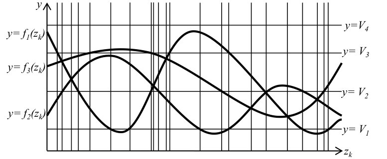 Figure 1
 Figure 2
 Figure 4
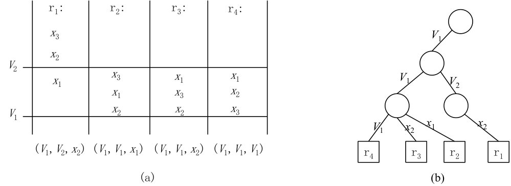 Figure 5
Peer Reviews
No public reviews on file for this paper yet. If you reviewed it on a platform where reviews are public (OpenReview, ICLR, NeurIPS, ICML), you can paste yours below so the community can read it here.
Videos
No videos yet. Explain this paper in a talk, walkthrough, or lecture? Add one.
Taxonomy
TopicsAlgorithms and Data Compression · DNA and Biological Computing · Computability, Logic, AI Algorithms
† HKUST, Hong Kong. ‡ Freie University‘̀at Berlin, Germany
\CopyrightSiu-Wing cheung and and Kai Jin
\EventEditors \EventNoEds1 \EventLongTitleAsian Association for Algorithms and Computation 2019 \EventShortTitleAAAC 2019 \EventAcronymAAAC19 \EventYear2019 \EventDateApril 19-21, 2019 \EventLocationSeoul, South Korea \EventLogo \SeriesVolume \ArticleNo1 \hideLIPIcs
A note on self-improving sorting with hidden partitions
Siu-Wing Cheng*†*
,
Man-Kwun Chiu*‡*
and
Kai Jin*†*
Key words and phrases:
Self-improving algorithm
1991 Mathematics Subject Classification:
Theory of computation
1. Introduction.
The sorting problem under a so-called “self-improving computational model” was studied in [1]: In this model, we will have input instances etc generated as follows. An instance contains elements , and its -th () element is generated according to a distribution . The distributions are fixed but are not given. The target is to compute and output – the ranks of the elements in .
Let denote the entropy of the output . The authors in [1] showed that they can design a learning phase which learns the distributions and builds some data structures by analyzing several instances so that for a given in the operation phase, they can compute in expected time, which matches the information theory lower bound.
We study in this paper a more general setting which allows some dependency among the elements. We assume that the elements are partitioned into groups (each element belongs to exactly one group) and in the -th () group there is a variable which is generated according to a fixed distribution and each element in this group is a function of . Note that the partition as well as the distributions are not given.
However, we need to impose some constraints on these functions of . Assume that the -th group contains elements and moreover . We assume that each function can have at most extremal points and every pair of functions and can have at most intersections, where and are known constants.
Under such constraints, our result is the following.
Theorem 1.1**.**
In operation phase, we can compute in expected time.
1.1. Technique overview
Learning phase overview.
We learn the hidden partition using constant many instances. Also, we construct the -list in the same way as in [1]. Precisely, take instances and merge all the elements in these instances into a big list and sort them in increasing order; denote the results by . Assign , , and . We call the predecessor of if . For the -th group, the predecessors of the elements in this group respectively and the order between these elements are denote by ; its entropy denoted by . Finally, let , and we sample instances to learn the distribution of .
Operation phase.
First, we compute for each . Second, for each , denote the list of elements in -th group in sorted order, find all such that is nonempty, and put the sublist into (So is a set of sublists). Third, we use a merge sort to merge all the sublists in into one list in sorted order. Finally, by concatenating , we obtain the sorted list of all elements.
1.2. Running time analysis of the operation phase.
We need the following three crucial lemmas.
Lemma 1.2**.**
For each , we can compute in time.
Lemma 1.3**.**
.
Lemma 1.4**.**
With high probability, on our construction of the -list, it is guaranteed that for each , the expected size of (i.e. the number of sublists in ) is a constant.
By Lemma 1.2, the first step runs in time, which is time further according to Lemma 1.3. The second and last step cost time. The third step takes time by applying Lemma 1.4. Thus we get Theorem 1.1.
Lemma 1.3 follows from Lemma 2.3 of [1] because we can compute in comparisons given . Lemma 1.4 is the same as Lemma 6 in [2]. Lemma 1.2 is proved below.
2. Learning phase I – compute the hidden partition in rounds
Assume we want to determine whether (, ) is in the same group.
Recall that each function has at most extremal points. We take samples of . Denote the values by . Without loss of generality, assume that . (Otherwise we make it so by sorting)
Moreover, for any sequence of numbers with length , we define function as the minimum number such that can be partitioned into monotonic sub-sequence. A sub-sequence is monotonic if it is either increasing or decreasing.
We can prove that
- •
If and are in the same group, ;
- •
If and are in different groups, .
Therefore,
- •
If , with high probability are in the same group.
- •
If , it is definitely true that are in different groups.
As a consequence, we can learn the hidden partition easily by calling function .
Moreover, since is a constant, so as , hence it only costs constant time to compute .
3. Learning phase II – learn the distribution of
We need to introduce some notation here.
For convenience, assume that are in the -th group.
First, we draw curves . Moreover, for each , we draw a horizontal line . Let denote the arrangement of these curves.
For each intersection in , we draw a vertical line, as shown in Figure 1. According to our assumption on the functions, there are less than such intersections. These intersections divide the plane into at most slabs. Notice that remains the same when is restricted to any fixed slab, yet it could be the same for different slabs. Thus there are at most possible (different) choices of , denoted by . Moreover, let be the probability that is identical to . Note that are all unknown and we do not build explicitly. Remind that the entropy is simply defined as .
In learning phase, we take instances to sample the results of and count their frequency. For , denote by the times that is sampled. Let . (Note that might be zero for some ; such is unknown to us. Other ’s are known.)
3.1. Store all the sampled results of in a trie
We encode every known result of by a vector (similar to the Lehmer code).
Definition 3.1**.**
Given a known result of , element is defined as among the predecessor of ; and is defined as among the predecessor of ; so on and so forth; finally, is defined as the predecessor of among .
Four examples are given in Figure 2 (a). The bottom of the columns shows the vectors.
We store the vectors of all sampled results of into a trie as shown in Figure 2 (b). Moreover, we assign every node in this trie a weight: A leaf labeled by has weight , and the weight of an internal node equals the total weight of its sons; so the root has weight 1.
4. Operation phase Step 1 – compute
First, let us consider an ideal case where , i.e. for every ,.
Assume we are given the values of and we want to determine . Equivalently, we want to determine the vector corresponding to . Similar as what Fredman did in [3], using , we can compute step by step. When , this process corresponds to a path in the trie starting from the root to the leaf labeled with .
According to some basic algorithmic knowledge (see section 3.2 paragraph 1 in [1]), if currently we are at a node with weight and the next round we proceed to a son with weight , the time for choosing the son in this step would be . Therefore, if , it takes time to reach the node labeled with .
Further since the probability that “” is , the expected time for computing would be when .
Next, we show that even if , the expected running time is still .
4.1. The proof of Lemma 1.2
Denote . Let be the time for computing when and when our sampling result is some fixed . Similar as in the above case, for , we compute in time when ; yet for , we find no result after searching the trie and we use a trivial method to compute and it costs time. Therefore,
[TABLE]
Thus the expected running time for computing in operation phase is given by
[TABLE]
[TABLE]
[TABLE]
[TABLE]
[TABLE]
To bound the first term, we need to bound , for which we apply the Chernoff bound. Note that the expectation of is given by , so . Hence .
To sum up, altogether we prove that the expected running time is .
The reference list from the paper itself. Each links out to its DOI / PubMed record.
- 1[1] N. Ailon, B. Chazelle, K. Clarkson, D. Liu, W. Mulzer, and C. Seshadhri. Self-improving algorithms. SIAM Journal on Computing , 40(2):350–375, 2011. doi:10.1137/090766437 . · doi ↗
- 2[2] S. Cheng and L. Yan. Extensions of self-improving sorters. In 29th International Symposium on Algorithms and Computation, ISAAC 2018, December 16-19, 2018, Jiaoxi, Yilan, Taiwan , pages 63:1–63:12, 2018. doi:10.4230/LIP Ics.ISAAC.2018.63 . · doi ↗
- 3[3] M.L. Fredman. How good is the information theory bound in sorting? Theoretical Computer Science , 1(4):355 – 361, 1976. doi:https://doi.org/10.1016/0304-3975(76)90078-5 . · doi ↗