Geodesic Structure of Naked Singularities in AdS$_3$ Spacetime
Cristi\'an Mart\'inez, Nicol\'as Parra, Nicol\'as Vald\'es, Jorge, Zanelli

TL;DR
This paper thoroughly analyzes the geodesic structure around naked singularities in AdS$_3$, providing explicit solutions and classifying geodesic behaviors, with implications for understanding spacetime geometry and particle trajectories.
Contribution
It offers a complete integration and classification of geodesics in AdS$_3$ naked singularity spacetimes, including explicit solutions and analysis of their properties.
Findings
Null and spacelike geodesics approach the singularity from infinity.
Timelike geodesics are bounded and do not always fall into the singularity.
Spatial geodesics can have self-intersections and circular orbits.
Abstract
We present a complete study of the geodesics around naked singularities in AdS, the three-dimensional anti-de Sitter spacetime. These stationary spacetimes, characterized by two conserved charges --mass and angular momentum--, are obtained through identifications along spacelike Killing vectors with a fixed point. They are interpreted as massive spinning point particles, and can be viewed as three-dimensional analogues of cosmic strings in four spacetime dimensions. The geodesic equations are completely integrated and the solutions are expressed in terms of elementary functions. We classify different geodesics in terms of their radial bounds, which depend on the constants of motion. Null and spacelike geodesics approach the naked singularity from infinity and either fall into the singularity or wind around and go back to infinity, depending on the values of these constants, except…
Click any figure to enlarge with its caption.
 Figure 1
 Figure 2
 Figure 3
 Figure 4
 Figure 5
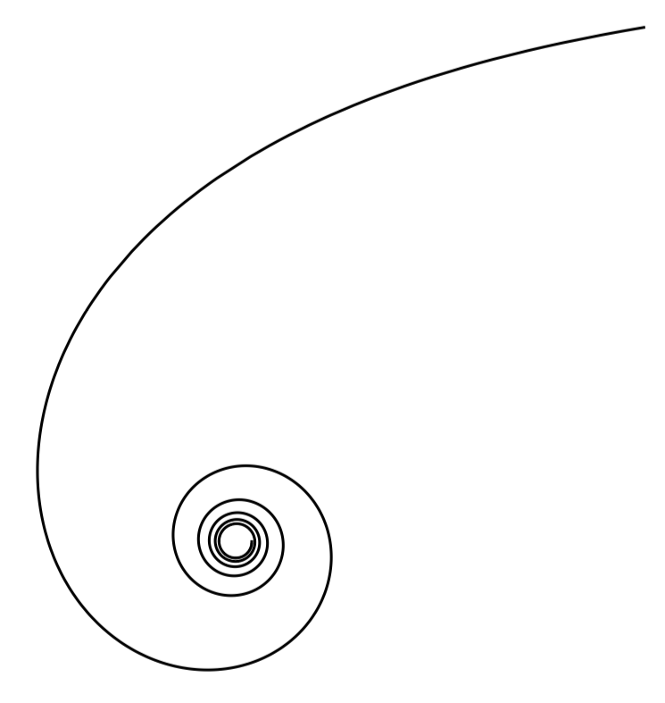 Figure 3
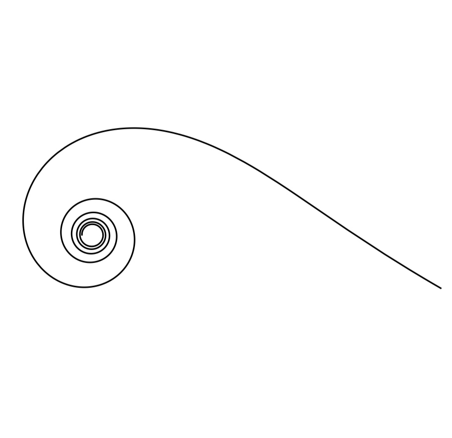 Figure 3
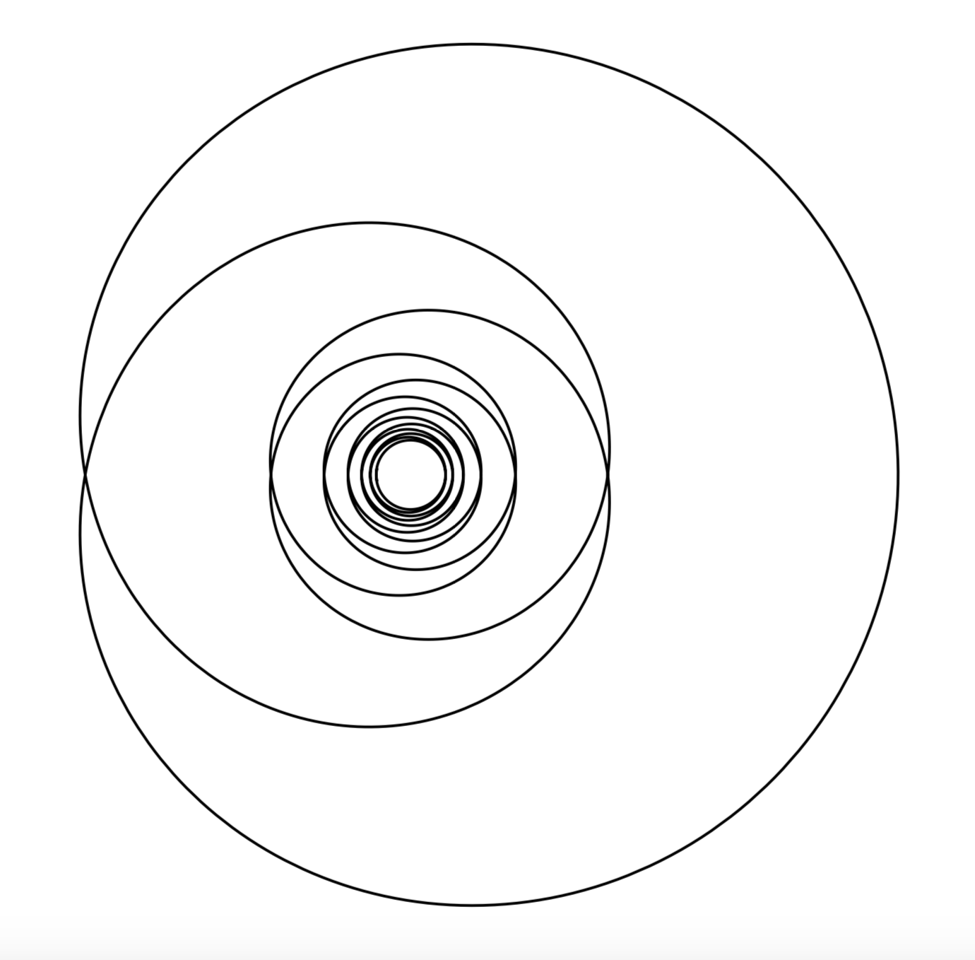 Figure 3
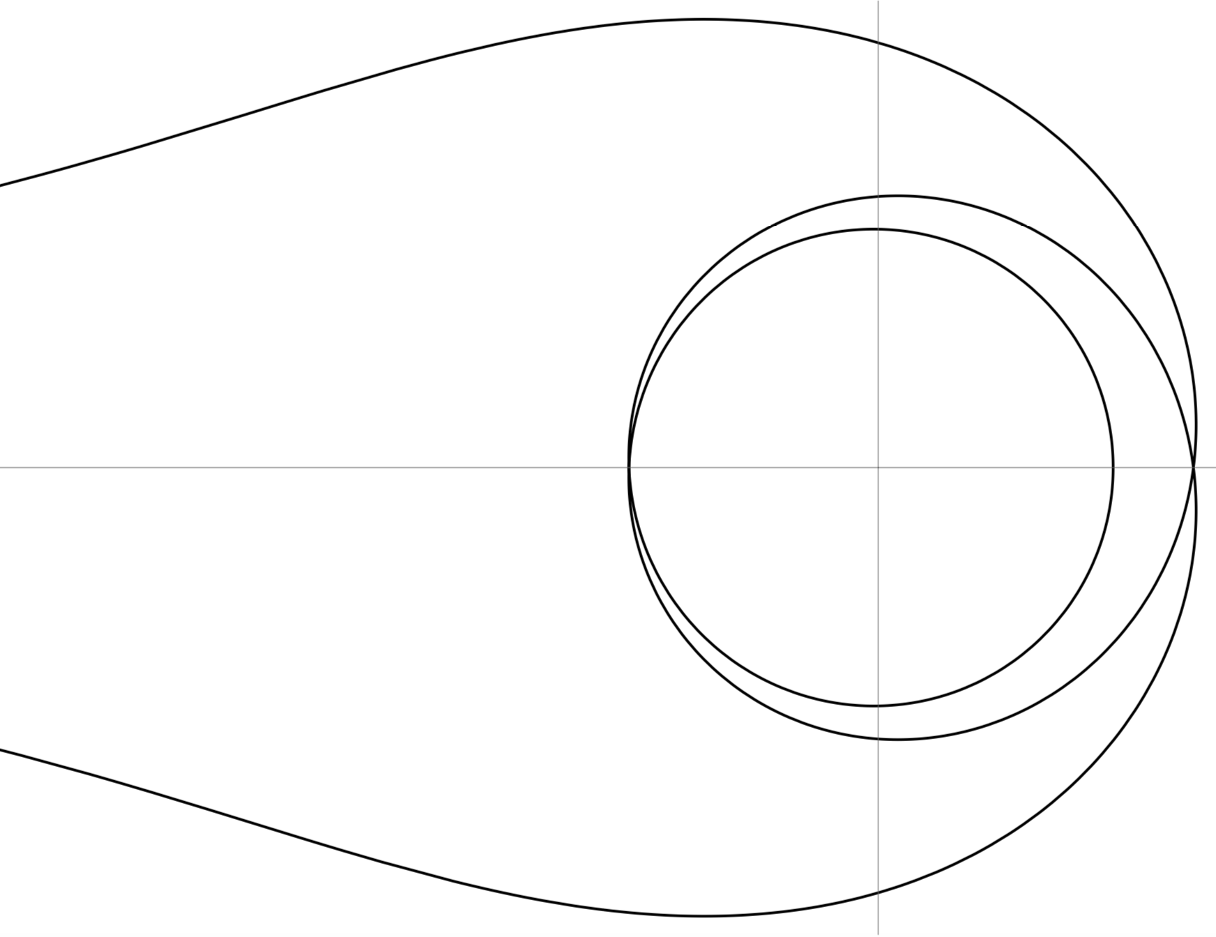 Figure 43
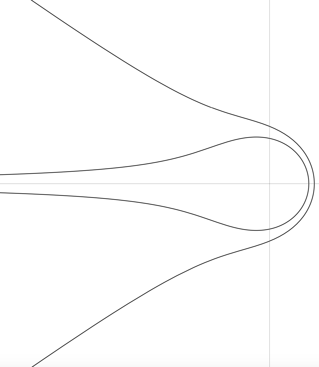 Figure 44
| - regions | Geometries |
|---|---|
| and | Black holes |
| and | Extremal black holes |
| and | Naked singularities |
| and | Extremal naked singularities |
| and | Massless BTZ geometry |
| and | AdS3 vacuum |
| Killing vector | Geometry |
|---|---|
| Generic NS () | |
| Extremal NS ( | |
| Massless BTZ geometry () |
| Range of and | Range of |
|---|---|
| , | constant and arbitrary |
| Cases | Range of |
|---|---|
| (a), (b) | |
| (c) |
| Cases | Range of |
|---|---|
| (b) | |
| (a), (c) |
| Case | Range of | |
|---|---|---|
| , | ||
| , | constant and arbitrary | |
| , | ||
| , | ||
| , | ||
| , |
Peer Reviews
No public reviews on file for this paper yet. If you reviewed it on a platform where reviews are public (OpenReview, ICLR, NeurIPS, ICML), you can paste yours below so the community can read it here.
Videos
No videos yet. Explain this paper in a talk, walkthrough, or lecture? Add one.
**Geodesic Structure of Naked Singularities
in AdS3 Spacetime
**
Cristián Martíneza, Nicolás Parrab, Nicolás Valdésb and Jorge Zanellia
a Centro de Estudios Científicos (CECs), Av. Arturo Prat 514, Valdivia, Chile.
b Departamento de Física, FCFM, Universidad de Chile, Blanco Encalada 2008,
Santiago, Chile.
[email protected], [email protected], [email protected], [email protected]
Abstract
We present a complete study of the geodesics around naked singularities in AdS3, the three-dimensional anti-de Sitter spacetime. These stationary spacetimes, characterized by two conserved charges –mass and angular momentum–, are obtained through identifications along spacelike Killing vectors with a fixed point. They are interpreted as massive spinning point particles, and can be viewed as three-dimensional analogues of cosmic strings in four spacetime dimensions. The geodesic equations are completely integrated and the solutions are expressed in terms of elementary functions. We classify different geodesics in terms of their radial bounds, which depend on the constants of motion. Null and spacelike geodesics approach the naked singularity from infinity and either fall into the singularity or wind around and go back to infinity, depending on the values of these constants, except for the extremal and massless cases for which a null geodesic could have a circular orbit. Timelike geodesics never escape to infinity and do not always fall into the singularity, namely, they can be permanently bounded between two radii. The spatial projections of the geodesics (orbits) exhibit self-intersections, whose number is particularly simple for null geodesics. As a particular application, we also compute the lengths of fixed-time spacelike geodesics of the static naked singularity using two different regularizations.
1 Introduction
Shortly after the BTZ black hole in three-dimensional spacetime was discovered [1, 2], its geodesic structure was studied in detail [3, 4]. The study of those geodesics not only gave insight into the geometrical properties of the BTZ spacetime, but also led to some interesting applications [5, 6, 7, 8].
The same BTZ metric, with mass and angular momentum , when continued to negative values of describes other interesting geometries. In the static case , for the resulting three-dimensional spacetime is a conical geometry with deficit angle and a naked singularity at the apex of the cone [9]. Naked singularities (NS) correspond to point particles, while geometries with angular excesses may be interpreted as antiparticles [10, 11]. These naked singularities can be viewed as the dimensional analogues of cosmic strings in dimensions and have been an object of extensive study in the past [12, 13]. Here we study the geodesics around these BTZ naked singularities (NS), extending to what is already known about the black holes.
From a geometric perspective, the NS in three-dimensional AdS spacetime can be obtained by identifying points along a rotational Killing vector. More precisely, one identifies with rotations on two independent planes in . Identifications in AdS3 have been used to describe black hole formation [14] and a construction of time machines [15]. In this paper we present all possible geodesics around of BTZ cones. Our analysis may contribute to an understanding of some aspects of current interests: specifically, these geodesics could be useful for discussing entanglement entropy [16, 17], and for recent studies of quantum backreaction on naked singularities [18, 19, 20, 21].
This paper is organized as follows. In Section 2 we review the NSs and discuss how to obtain them by identifications on the covering AdS3 space embedded as a pseudo-sphere in . In Section 3 we use conserved quantities along geodesics to find the first order geodesic equations in NS spacetimes, and then through re-scaling write the equations in a convenient form. In Section 4, we present solutions to the radial equations and corresponding bounds for the different types of geodesics. We note that all null geodesics escape to infinity or fall into the singularity, except for a special case which allows circular orbits. Similarly, spacelike geodesics either have both ends at infinity, or one end at infinity and the other at the singularity. Meanwhile, all timelike geodesics are bounded: they either orbit the NS at finite radius or fall into it. Section 5 deals with the spatial projections of the geodesics. We find exact analytic solutions, plot representative orbits and discuss their qualitative behavior. In Section 6, we analyze an interesting property of the geodesics arising from the results of Section 5: null, spacelike, and timelike geodesics can all intersect themselves, and we calculate the number of self-intersections. Section 7 presents two more properties: the time behavior of geodesics, and the lengths of spacelike geodesics. The last section contains a summary and discussion of the main results.
2 The NS spacetime
Although all vacuum solutions of the three-dimensional Einstein equations with negative cosmological constant are constant curvature spacetimes locally isometric to AdS3, there exist geometries globally distinct from AdS3, including black holes. This is the case of the family of BTZ geometries described by the stationary line element
[TABLE]
where , , , and . Here the mass and angular momentum are integration constants111We set the three-dimensional Newton constant as .. Depending on the values of and various spacetimes emerge from the BTZ metric (2.1), which are summarized in Table 1.
Here we are interested in the naked singularities (with ), namely, the geometries without an event horizon, which correspond to spacetimes with nonpositive mass . The only exception is the case , which is the AdS3 spacetime. NSs can be obtained by identifications on the universal covering space CAdS3 [9]. We present below a brief review of this construction.
Consider CAdS3 as the set of points of the pseudo-sphere embedded in defined by
[TABLE]
This embedding can be parametrized with coordinates on the hypersurface defined by (2.2), which yields the induced metric (2.1). The Killing vector is chosen as the identification vector and is written as a linear combination of the generators ,222Here , with .
[TABLE]
where the antisymmetric matrix characterizes the identification in terms of the generators. Then, the action of the matrix on the coordinates of the embedding space is
[TABLE]
The explicit form of the embeddings for the different geometries and the corresponding identification matrices can be found in Refs. [9, 21]. The different identification vectors are shown in Table 2, where we have defined
[TABLE]
As Table 2 displays, the non-extremal NS is obtained by an identification by a Killing vector formed by two rotations. Note that for the extremal and massless cases, the Killing vectors contain rotations and boosts that are not limiting cases of the generic form.
3 Geodesic equations
The NS spacetimes have two Killing vectors and . They provide two conserved quantities along the geodesic motion, and , respectively, where is tangent to the geodesic with affine parameter . This allows us to obtain the first integrals
[TABLE]
Since the velocity can be normalized as (with for null geodesics, for timelike geodesics, and for spacelike geodesics), one gets
[TABLE]
Equations (3.1-3.3) are exactly the same for black holes () [4] and naked singularities (). However, the denominators of and vanish at the BH horizons, while for NS they are positive definite. Consequently, the geodesics around a NS are drastically different from those in the BH case.
Using (2.5) it is convenient to write
[TABLE]
and since and , it is useful to introduce the following quantities333The massless BTZ spacetime is considered separately in 4.4.
[TABLE]
Furthermore, for we use the rescaled quantities
[TABLE]
with . Then, omitting the tildes hereafter, the geodesic equations read
[TABLE]
The solutions of these equations contain three integration constants and . Due to the invariance under rotations and time translations, and can be chosen to vanish without loss of generality.
4 Radial bounds
The equation for the radial motion (3.9) is conveniently written as
[TABLE]
with
[TABLE]
Geodesics exist in the regions where is non-negative. With this criterion one can find radial bounds for the different geodesics. It is important to note that for timelike and null geodesics, would imply and , which in turn implies for all . Hence, is a necessary condition for the existence of timelike and null geodesics, although not for spacelike ones.
In what follows, we analyze the -dependence of the different types of geodesics, first for generic and separately for .
4.1 Null geodesics ()
The existence of null geodesics for non-extremal NSs requires , and since , it is useful to define
[TABLE]
which verifies . Under this condition on the region where is non-negative depends on the sign of . In the case null geodesics are allowed for . Alternatively, for the null geodesics are permitted in the half line . Table 3 summarizes the possible ranges of for null geodesics around a naked singularity.
Integrating Eq. (4.1) with , we obtain
[TABLE]
Note that for the minimum of the parabola given by (4.4) is non-positive, which implies that any null geodesic coming from a finite radius reaches at a finite value of . Hence, these null geodesics have no turning point. Meanwhile, in the case there is a non-zero turning point at
[TABLE]
as shown in Table 3.
For the extremal naked singularity (), the cases and are not allowed for null geodesics. Remarkably, for , Eq. (4.1) provides the circular null geodesics constant, where any radius is permissible. For , null geodesics are allowed for if or , and have a turning point if , as shown in Table 3.
4.2 Timelike geodesics ()
Timelike geodesics exist in the regions where the quadratic function in (4.1), defined in the domain , is non-negative. In cases (a) and (b) , , the function is non-negative in the interval , where
[TABLE]
Note that under conditions (a) or (b), the discriminant is always positive. A third case is defined by the condition (c) . Here in the interval . On the other hand, timelike geodesics are not possible for the cases , or , .
For the static NS (), timelike geodesics with satisfy condition (c), since , and thus do not fall into the singularity. The radial timelike geodesics () satisfy condition (b).
The radial equation (4.1) for is integrated as
[TABLE]
which agrees with the cases (a), (b) and (c) previously discussed. In the extremal NS, the cases or , are also not allowed for timelike geodesics. For the bounds shown in Table 4 are obtained under the condition . Equation (4.7) also holds for the extremal NS.
4.3 Spacelike geodesics ()
For spacelike geodesics, becomes a convex parabola. In the analysis of radial bounds there are three cases to consider:
(a) For and , the geodesics stretch from infinity to a minimum radius .
(b) For and , all geodesics end at the singularity.
(c) For and , once again the geodesics can be in the region . It can be shown that is incompatible with , so we do not consider this case.
Solving Eq. (4.1) with yields
[TABLE]
It can be verified that this solution satisfies the bounds mentioned earlier as summarized in Table 5. This table also provides radial bounds for the extremal case , for which the solution (4.8) holds as well.
A qualitative summary of the results for radial bounds is that null and spacelike geodesics approach the NS from infinity, and either fall into the singularity or wind around and go back to infinity (with the exception of the extremal case for which a null geodesic with has a circular orbit). Meanwhile timelike geodesics either orbit continually bounded between two radii, or fall into the NS.
4.4 Geodesics on the massless BTZ geometry
The geodesic equations for the massless BTZ spacetime (), written in terms of the original variables444In this case the rescalings (3.6) are no longer valid. of Eqs. (3.1)(3.3), are given by
[TABLE]
The integration of these equations is straightforward and Table 6 summarizes the solutions of the radial equation and bounds. Note that provides radial geodesics and the case is not allowed for null and timelike geodesics. Moreover, the bounds match those for in the limit , c.f. [4].
In the null case (), for , we obtain
[TABLE]
where is an arbitrary integration constant. The range of the affine parameter is for the upper sign, and for the lower sign. For , is constant (circular orbit).
For the timelike case (), the solution of the radial equation is given by
[TABLE]
with , i.e., is bounded.
Finally, for spacelike geodesics (), the solution of the radial equation is
[TABLE]
where the upper (lower) sign corresponds to outgoing (ingoing) geodesics. For , the range of the affine parameter is for outgoing geodesics, and for the incoming case. Otherwise, if , the affine parameter can take all real values.
5 Orbits in the - plane
Now, we analize the orbit equation , which can be obtained from (3.8) and (3.9). Once again we begin with the non-extremal case. Integration of the orbit equation yields
[TABLE]
with
[TABLE]
and
[TABLE]
where and .
For null and timelike geodesics, holds, so . Then, in the sub-case , Eq. (5.1) reduces to . On the other hand, is allowed for a spacelike geodesic, and in this case .
In the static case (), Eq. (3.8) gives the radial geodesic for . Note that there are no radial geodesics if , i. e., rotating NSs always produce dragging.
Null geodesics with have the simple expression
[TABLE]
which has a turning point at . For timelike and spacelike geodesics,
[TABLE]
in agreement with the radial bounds shown for condition (c) in Table 4. In the limit , Eq. (5.5) matches the orbit for the static null geodesics (5.4). Note that the integration constant here has been chosen as , unlike in (5.1), to make the expression (5.5) simpler.
We include plots that help visualize the different geodesics. Note in particular the possibility of null geodesics to reach infinity. Additionally, the winding of geodesics near the NS can either be increased or decreased, depending on the magnitude of and its sign relative to . This dragging produced by the rotation of the NS, can be seen in figures 1(a) and 1(b).
As we adjust different parameters (in particular, ), the number of times geodesics wind around the NS and intersect themselves changes. This winding phenomenon is studied in detail in the following section.
In agreement with the solutions discussed in the previous section, timelike geodesics follow bounded orbits around the NS. For and rational values of , the orbits are closed. As the denominator of (expressed as an irreducible fraction) grows, timelike geodesics take more winds to close. Figure 2(c) is an example of the failure of timelike geodesics to close when is irrational. In this figure is not allowed to cover its entire range, for otherwise nothing would be visible.
The extremal naked singularity produces different solutions for orbits. For null geodesics the orbit equation is defined only if and the solutions are is
[TABLE]
As for timelike and spacelike geodesics, we have
[TABLE]
We note that can always be chosen to be positive for the null and timelike cases, as will be discussed in Section 7.
5.1 Orbits for the massless BTZ geometry
Finally we consider orbits in the massless BTZ spacetime. The non-radial () and non-circular () orbits for all geodesics are given by
[TABLE]
where can be set as , or [math].
For null or spacelike geodesics and , this equation describes a spiral connecting with . Additionally, there is a reflected spiral due to the symmetry of Eq. (5.8) (not shown in Fig. 3).
Timelike geodesics –which require – are spirals connecting the origin for to a maximum finite radius at . Then, after an infinite number of turns they return to the origin for . Note that as shown in Eq. (4.11), the entire geodesic is covered by an affine parameter that is bounded for timelike geodesics of the massless BTZ spacetime. Although the radial motion for a timelike geodesic (4.11) is sinusoidal, it does not describe an oscillation near the singularity.555This point was incorrectly interpreted in [5]. In Figure 3 we illustrate each type of geodesic. Globally they are quite different, though close to the singularity all geodesics simply look like the aforementioned spirals.
The case for spacelike geodesics is also considered in (5.8), but here the geodesics do not reach the singularity. Instead they have a finite minimum radius as indicated in Sec. 4.4. In these spacelike geodesics is bounded as , where
[TABLE]
is the angle for . If , the geodesic comes from infinity and goes back to infinity without self-intersections. For the geodesic wind around the singularity a number of times before going back to infinity. This behavior is illustrated with two examples in Figure 4.
6 Self-intersections
Null and spacelike geodesics that have a turning point intersect themselves. These geodesics start at infinity and wind around the singularity a finite number of turns, reach the turning point and go back to infinity after repeating the same number of turns. The number of self-intersections is the integer number of times that is contained in the angle swept by the geodesic as goes from to and back to . First, we count self-intersections for .
Let us consider null geodesics with a turning point , which require and . Setting the angle at equal to 0, then at it is
[TABLE]
Since and , we have . Moreover, if we have and therefore,
[TABLE]
The number of self-intersections () is the integer part of , except for , in which case one must subtract 1 (which corresponds to a self-intersection at ). Hence, this number is given by
[TABLE]
where the ceiling function is the least integer greater than or equal to , and . The difference between and for a given sign of is due to the fact that the rotating background breaks the clockwise/counter-clockwise symmetry of the null geodesic. Once again, we see that the rotation of the NS can either increase or decrease the winding of the geodesic.
For the extremal case, self-intersections occur only if , then we get
[TABLE]
We can also obtain the winding number for spacelike geodesics, which start at infinity and reach a minimum radius, as . Assuming in (5.3), the angle at the turning point is given by
[TABLE]
From this it is relatively straightforward to show that
[TABLE]
while at one finds,
[TABLE]
As explained in Section 5, if only the second terms in (6.6) and (6.7) must be considered, while if just the first ones appear in those expressions.
Self-intersections are also present in timelike orbits. They occur in case (c) of Table 4, where timelike geodesics are bounded by two radii. However, in general orbits do not close which leads to an infinite number of intersections (see for instance Figure 2(c)).
For the massless BTZ spacetime, self-intersections occur for time- and spacelike geodesics. Initially outgoing timelike geodesics with (see Figure 3(c)) can have an arbitrarily large number of self-intersections depending on the initial conditions; for spacelike geodesics with (see Figure 4(b)), using in Eq. (5.9), the number of the self-intersections is found to be
[TABLE]
It is worth noting that the number of self-intersections for null geodesics depends only on the spacetime quantities and , while for spacelike and timelike geodesics, the number of self-intersections also depends on the constants of the orbit and .
7 Additional features
7.1 The time coordinate
So far we have not discussed the behavior of the time coordinate for geodesics in the NS spacetimes. We note, firstly, that the equation of motion (3.7) for closely resembles equation (3.8) for . Indeed, integrating (3.7) gives a very similar expression to (5.1),
[TABLE]
where
[TABLE]
and are given by (5.3).
Another aspect of the time coordinate worth noting is the sign of throughout a trajectory. We can see from the geodesic equation (3.7) that could change sign at . However, this does not occur for timelike or null geodesics, which can be seen as follows:
i) Null geodesics are either radial or never reach the singularity and have a turning point at . Hence, massless particles never reach the point, and the sign of for their geodesics is constant.
ii) For timelike geodesics it can be shown that in Eq. (4.1), and therefore lies outside of the allowed range for .
Additionally, from Eq. (3.7) note that as , and thereore, without loss of generality one can always choose and so that is monotonically increasing for timelike and null geodesics. This means that there are no closed timelike geodesics in a NS spacetime in AdS3 [2]. On the other hand, for spacelike geodesics no such restrictions exist and both and can have any sign, and could even vanish for the entire geodesic.
7.2 Lengths of spacelike geodesics
The lengths of spacelike geodesics have been relevant for some time now due to the Ryu-Takayanagi (RT) prescription for computing entanglement entropy from the area of minimal surfaces [16]. The relevant geodesic is a purely spatial curve and therefore we consider the spacelike geodesics with and . The length of a geodesic arc is given by . Then, the arc length of a geodesic path that sweeps out an angle in going from back to is,
[TABLE]
where corresponds to the minimum radius. The integration yields666In the original variables, save for a re-scaling of by . Here, , with .,
[TABLE]
where satisfies
[TABLE]
As could be expected, expression (7.4) diverges. To give physical meaning to this length it is necessary to regularize it by subtracting off another divergent length. In this case, a reasonable choice is to compare with the corresponding geodesic length in AdS3 , which in a sense corresponds to the vacuum geometry. A problem is that there can be different meanings for “corresponding geodesics” between different spacetimes. One can choose geodesics that have the same parameters and , or that sweep the same angle . These two options lead to different results. Indeed, comparing geodesics of the same (and ) leads to
[TABLE]
i.e., the length of spacelike geodesics with and the same angular momentum are equal in a NS spacetime as in AdS. On the other hand, comparing geodesics that sweep the same angle gives
[TABLE]
To arrive at this expression, the regularization leading to (7.6) is obtained as
[TABLE]
where is defined by Eq. (7.5), and is defined analogously but for . Thus, in order to subtract the limits, one must make an appropriate change of variables first. The two expressions (7.6) and (7.7) could be thought of as arising in different thermodynamic ensembles: in the first case the angular momentum is held fixed, while in the second its canonical conjugate (the angle ) is fixed.
Our results for differ from those found by other authors. For instance, the expression for in Eq. (2.5) of [17] (with ) in our notation reads
[TABLE]
where is a regulator and the discrepancy may be attributed to the different regularization prescription.
The expression (7.7) naturally vanishes for but yields a finite result in the limit , which would not match the vanishing entropy of a massless BTZ black hole. In contrast with this, (7.9) diverges for but gives a non vanishing result for AdS, which means that that regularization corresponds to comparing with a different geometry. The result (7.6), on the other hand, seems reasonable if the NS geometry is viewed as a point particle that has no horizon and therefore no Hawking temperature and no entropy. There is an additional difficulty with the interpretation of (7.7): Since the NS geometry is obtained by removing an angular sector from AdS, this renders uncertain the idea of comparing lengths with the same opening angle in the two geometries. For instance, it is not clear what happens if the removed angle is larger than .
8 Conclusions and discussion
We have investigated the geodesic structure of NS in three-dimensional anti-de Sitter spacetime. We found that null and spacelike geodesics have a finite number of self-intersections. This occurs when they do not reach the singularity, but rather start and end at infinity. For null geodesics the number of self-intersections is a simple expression that depends only on properties of the spacetime ( and ), independently of the values of the particular geodesic. On the other hand, for spacelike geodesics the number of self-intersections depends on the constants as well. Timelike geodesics have bounded orbits and also intersect themselves, but this behavior is more complicated, as shown in Figure 2. For example, for the static NS the orbits do not close unless is a rational number. When they do not close, they have an infinite number of self-intersections.
It is interesting to point out differences and similarities with the case. For the black hole, the dependence of on is logarithmic and no self-intersections are present. For the black hole, massive particles always fall into the singularity, while for the NS this does not happen in case (c) of Table 4 (see also Figure 2). Null geodesics can escape the singularity for both black holes and NS, but radial bounds are complementary: if a null geodesic has parameters such that it reaches the NS, a geodesic with those same parameters will not reach the black hole singularity. Conversely, a null geodesic that reaches the black hole singularity would not fall into the NS.
Our results can be related to a recent observation which shows that in the presence of a conformally coupled scalar field, the naked singularity in dimensions becomes surrounded by a “quantum dress” [18, 19, 20, 21], which could be a physical mechanism for realizing the cosmic censorship conjecture [22]. In the static case, the Green functions in the NS spacetime can be constructed using the method of images, since the conical singularity is obtained by identifications in AdS3. The number of images to be summed over is in correspondence with the number of self-intersections of the null geodesics calculated here. This last statement can be understood pictorially as follows: to compute Green functions one needs the geodesic distance between two points. If null geodesics in a spacetime have self-intersections, any two infinitesimally close points can be joined by topologically distinct null geodesics and to compute the two-point function, one must sum over all of these geodesics. Hence, there is a correspondence between this number and the number of images of a point under the identification used to get a NS from AdS3.
Another application lies in the study of entanglement entropy of the dimensional CFT dual of the NS in dimensions. In this analysis, according to the RT conjecture, the length of the minimal spatial geodesics play a central role [16]. In Section 7 we computed these lengths comparing them to the corresponding geodesics in AdS3, and found different results depending on which ensemble we considered: if the corresponding geodesics have the same value of the regularized length vanishes; if the corresponding geodesics have the same value of the result is nonzero. Neither of these results match the finding in [17].
There are related questions that we have not touched upon, but that could be considered in the future. For instance, a similarly detailed study of multiple conical singularities could be carried out. Moreover, if one considers identifications of AdS3 different from the one considered here using a spacelike Killing vector, it is possible to build other spacetimes [14, 15] and study their corresponding geodesics.
Acknowledgements
We are grateful to M. Briceño, M. Casals, B. Czech, A. Fabbri, G. Giribet and A. Ireland for enlightening discussions. This work has been partially funded by Fondecyt grants 1161311 and 1180368. The Centro de Estudios Científicos (CECs) is funded by the Chilean Government through the Centers of Excellence Base Financing Program of Conicyt.
The reference list from the paper itself. Each links out to its DOI / PubMed record.
- 1[1] M. Bañados, C. Teitelboim and J. Zanelli, The Black hole in three-dimensional space-time , Phys. Rev. Lett. 69 , 1849 (1992).[hep-th/9204099]. doi:10.1103/Phys Rev Lett.69.1849
- 2[2] M. Bañados, M. Henneaux, C. Teitelboim and J. Zanelli, Geometry of the (2+1) black hole , Phys. Rev. D 48 , 1506 (1993). [gr-qc/9302012]. Erratum: [Phys. Rev. D 88 , 069902 (2013) doi:10.1103/Phys Rev D.48.1506, 10.1103/Phys Rev D.88.069902
- 3[3] C. Farina, J. Gamboa and A. J. Seguí-Santonja, Motion and trajectories of particles around three-dimensional black holes , Class. Quant. Grav. 10 , L 193 (1993) doi:10.1088/0264-9381/10/11/001 [gr-qc/9303005].
- 4[4] N. Cruz, C. Martínez and L. Peña, Geodesic structure of the (2+1) black hole , Class. Quant. Grav. 11 , 2731 (1994). [gr-qc/9401025]. doi:10.1088/0264-9381/11/11/014
- 5[5] J. Troost, Winding strings and Ad S(3) black holes, JHEP 0209 , 041 (2002) doi:10.1088/1126-6708/2002/09/041 [hep-th/0206118].
- 6[6] J. V. Rocha and V. Cardoso, Gravitational perturbation of the BTZ black hole induced by test particles and weak cosmic censorship in Ad S spacetime, Phys. Rev. D 83 , 104037 (2011) doi:10.1103/Phys Rev D.83.104037 [ar Xiv:1102.4352 [gr-qc]].
- 7[7] A. Dasgupta, H. Nandan and S. Kar, Geodesic flows in rotating black hole backgrounds, Phys. Rev. D 85 , 104037 (2012) doi:10.1103/Phys Rev D.85.104037 [ar Xiv:1202.5370 [gr-qc]].
- 8[8] N. Tsukamoto, K. Ogasawara and Y. Gong, Particle collision with an arbitrarily high center-of-mass energy near a Bañados-Teitelboim-Zanelli black hole, Phys. Rev. D 96 , no. 2, 024042 (2017) doi:10.1103/Phys Rev D.96.024042 [ar Xiv:1705.10477 [gr-qc]].