On the Numerical Solution of the Exact Factorization Equations
Graeme H. Gossel, Lionel Lacombe, Neepa T. Maitra

TL;DR
This paper demonstrates a self-consistent numerical solution to the exact factorization equations, revealing their stability properties and implications for non-adiabatic molecular dynamics simulations.
Contribution
It introduces a novel approach to solve the EF equations self-consistently, addressing stability issues due to their non-Hermitian form.
Findings
Stable propagation achieved in model systems
Identification of non-Hermitian Hamiltonian effects
Insights into non-adiabatic dynamics modeling
Abstract
The exact factorization (EF) approach to coupled electron-ion dynamics recasts the time-dependent molecular Schr\"odinger equation as two coupled equations, one for the nuclear wavefunction and one for the conditional electronic wavefunction. The potentials appearing in these equations have provided insight into non-adiabatic processes, and new practical non-adiabatic dynamics methods have been formulated starting from these equations. Here we provide a first demonstration of a self-consistent solution of the exact equations, with a preliminary analysis of their stability and convergence properties. The equations have an unprecedented mathematical form, involving a non-Hermitian Hamiltonian, and so the usual numerical methods for time-dependent Schr\"odinger fail when applied in a straightforward way to the EF equations. We find an approach that enables stable propagation long enough to…
Click any figure to enlarge with its caption.
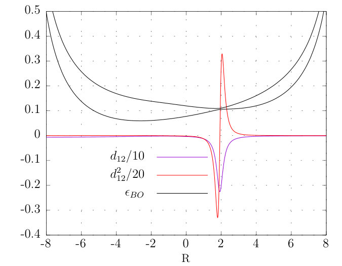 Figure 1
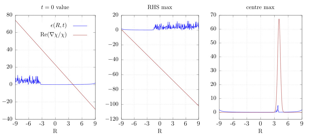 Figure 2
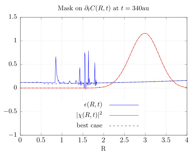 Figure 3
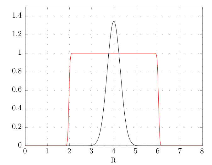 Figure 4
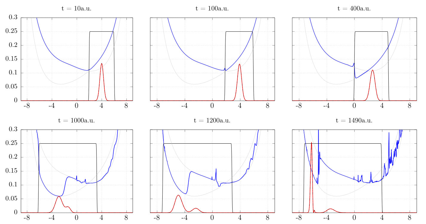 Figure 5
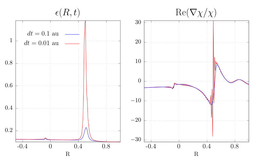 Figure 6
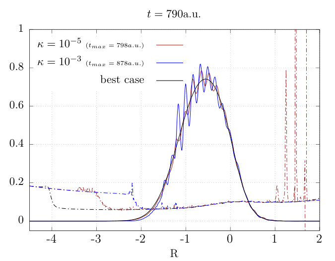 Figure 7
Peer Reviews
No public reviews on file for this paper yet. If you reviewed it on a platform where reviews are public (OpenReview, ICLR, NeurIPS, ICML), you can paste yours below so the community can read it here.
Videos
No videos yet. Explain this paper in a talk, walkthrough, or lecture? Add one.
On the Numerical Solution of the Exact Factorization Equations
Graeme H. Gossel
Department of Physics and Astronomy, Hunter College and the City University of New York, 695 Park Avenue, New York, New York 10065, USA
Lionel Lacombe
Department of Physics and Astronomy, Hunter College and the City University of New York, 695 Park Avenue, New York, New York 10065, USA
Neepa T. Maitra
Department of Physics and Astronomy, Hunter College and the City University of New York, 695 Park Avenue, New York, New York 10065, USA
The Physics Program and the Chemistry Program of the Graduate Center, City University of New York, 365 Fifth Avenue, New York, USA
Abstract
The exact factorization (EF) approach to coupled electron-ion dynamics recasts the time-dependent molecular Schrödinger equation as two coupled equations, one for the nuclear wavefunction and one for the conditional electronic wavefunction. The potentials appearing in these equations have provided insight into non-adiabatic processes, and new practical non-adiabatic dynamics methods have been formulated starting from these equations. Here we provide a first demonstration of a self-consistent solution of the exact equations, with a preliminary analysis of their stability and convergence properties. The equations have an unprecedented mathematical form, involving a non-Hermitian Hamiltonian, and so the usual numerical methods for time-dependent Schrödinger fail when applied in a straightforward way to the EF equations. We find an approach that enables stable propagation long enough to witness non-adiabatic behavior in a model system before non-trivial instabilities take over. Implications for the development and analysis of EF-based methods are discussed.
I Introduction
The exact factorization (EF) of the time-dependent molecular Schrödinger equation Abedi et al. (2010, 2012) is an exact reformulation of the quantum dynamics of interacting electronic and nuclear systems. The molecular wavefunction is expressed as a single product of a nuclear wavefunction and an electronic wavefunction that is conditionally dependent on the nuclear coordinate, with two coupled equations describing their motion. Many interesting exact properties of the formalism have been uncovered in recent works, e.g. Abedi et al. (2010, 2012); Suzuki et al. (2014); Khosravi et al. (2015); Abedi et al. (2013a); Min et al. (2014); Curchod et al. (2016); Fiedlschuster et al. (2017); Requist et al. (2016, 2017); Curchod and Agostini (2017); Lefebvre (2015); Agostini and Curchod (2018); Scherrer et al. (2017); Eich and Agostini (2016); Schild et al. (2016); Requist and Gross (2016); Li et al. (2018); Cederbaum (2015); Hoffmann et al. (2018); Schild and Gross (2017); Gonze et al. (2018), shedding light on the nature of interactions between dynamical quantum subsystems as well as on interactions between quantum and classical subsystems beyond adiabatic treatments. From a practical viewpoint, the EF equations provide a rigorous starting point for methods for non-adiabatic dynamics and already we have seen the development of mixed quantum-classical approaches Agostini et al. (2016); Min et al. (2015); Gossel et al. (2018); Agostini et al. (2018), with successful applications in photochemical dynamics Min et al. (2017), as well as density functionalizations Requist and Gross (2016); Li et al. (2018).
Regarding the exact EF equations, prior studies of the exact features were based on first solving the original full molecular Schrödinger equation, and then extracting the exact coupling terms from inverting the exact EF equations. That is, a direct numerical solution of the coupled exact EF equations was avoided. Indeed, the stability and convergence properties of these equations remained unexplored, properties which are of interest when developing further EF-based approximations. In this paper, we discuss unique challenges that a self-consistent numerical solution of the exact coupled EF equations pose, give a numerical solution for a model problem, and present a preliminary analysis of their stability. We show that the usual numerical methods developed for the time-dependent Schrödinger equation fail when applied to the EF equations, and investigate these failures with a preliminary formal analysis. We show how we were able to obtain a stable numerical propagation for long enough to witness non-adiabatic behavior in the model system before non-trivial instabilities kill the calculation.
This paper is structured as follows: section II briefly reviews the EF formalism. Section III then discusses aspects that a numerical solution need to consider, before discussing such a solution for a model problem in Sec. IV. A preliminary analysis of the well-posedness of the EF equations is given in Sec. V, before we conclude in Sec. VI.
II The exact factorization equations
In the EF approach Abedi et al. (2010, 2012); Gidopoulos and Gross (2014); Hunter (1975, 1981), the exact molecular wavefunction is written as a single product of a marginal wavefunction and a conditional wavefunction , as
[TABLE]
subject to the partial normalization condition (PNC)
[TABLE]
Here, represent the set of all nuclear coordinates and the electronic coordinates. The factorization above is unique up to phase-transformation that depends only the nuclear coordinates and time:
[TABLE]
Notice that Eq. (1) has the same form as the wavefunction in the Born-Oppenheimer approximation, but Eq. (1) is exact, as proven in the earlier works, and the equations that the two parts and satisfy differ from that in the Born-Oppenheimer equation. These equations may be derived by inserting Eq. (1) into the Dirac-Frenkel action and applying the variational principle Abedi et al. (2010, 2012, 2013b); Alonso et al. (2013), and, for one nuclear degree of freedom and one electronic degree of freedom have the form
[TABLE]
[TABLE]
where time-dependent potential energy surface (TDPES) , vector potential , and coupling operator are given by
[TABLE]
with indicating an inner product only over the electronic space. The potentials and represent potentials that are externally applied to the coupled system of electrons and nuclei, e.g. a laser field, and is the usual Born-Oppenheimer Hamiltonian consisting of electronic kinetic energy, electron-electron, electron-nuclear, and nuclear-nuclear Coulomb potentials. Note that atomic units are used throughout, and denotes the effective mass of the nuclear coordinate. Under the phase-transformation of Eq. (II), the potentials and transform in a gauge-like way:
[TABLE]
The TDPES can be separated into a gauge-independent (GI) term and a gauge-dependent (GD) term, where and are the remaining terms of Eq. (6). The three terms in Eqs. (6)– (8) capture the entire coupling of the electrons and nuclei; through them, the solution of the electronic equation depends on the nuclear wavefunction, and the solution of the nuclear wavefunction depends on the electronic wavefunction. Refs. Abedi et al. (2010, 2012, 2013a); Agostini et al. (2015); Min et al. (2014); Requist et al. (2016); Curchod and Agostini (2017) (for example), have emphasized the significance of and in yielding the exact nuclear dynamics; in contrast to the Born-Huang expansion, which is also exact, here the exact nuclear dynamics is achieved with a single potential energy surface rather than an infinite number of them, and a single vector potential coupling rather than an infinite number of first and second-order couplings. Wavepacket branching and decoherence are captured, where a central role is played by .
III A Priori Numerical Considerations
Here we make some observations that will inform our attempt to solve Eqs. (4) – (8) self-consistently for a model system.
III.1 Reality of potentials and
The equation for the nuclear wavefunction is of Schrödinger-form provided the potentials and are real. The reality of the potentials ensures that the Hamiltonian in the nuclear equation is Hermitian and consequently that the norm of the nuclear wavefunction is preserved during the time-evolution. However, the potentials and are determined by the solution of the electronic equation, which not only does not have a Schrödinger form, but has a Hamiltonian to which notions of hermiticity do not technically apply (see also Sec. III.2). Nevertheless, norm-conservation in the electronic equation is still a meaningful concept; indeed it is particularly important for the electronic equation, given the role of the PNC of Eq. (2) in ensuring that the factorization is unique. Propagation under the exact EF equations does conserve the partial norm Alonso et al. (2013); Abedi et al. (2013b) and in this subsection we show how this directly ensures the scalar and vector potentials that drive the nuclear equation are real. When the equations are discretized in a numerical simulation, additional considerations need to be made.
To see why the partial norm condition of the electronic wavefunction assures us that the scalar and vector potentials in the Schrödinger equation for the nuclear wavefunction are real, we first observe that
[TABLE]
where could represent or , i.e. a parameter of the electronic wavefunction. So the expectation value on the right-hand-side will be purely real if the PNC is satisfied. Taking , the expectation value appearing on the right-hand-side becomes the vector potential and hence PNC condition ensures is real. Taking , the expectation value on right-hand-side becomes the gauge-dependent part of the scalar potential, , hence the PNC condition ensures is real. The first two terms in the gauge-independent part are real due to the operators and being Hermitian, while the last term can be shown to be upon making use of the definition of the vector potential to cancel some terms. Thus, we have shown that the potentials and appearing in the Schrödinger equation for the nuclear wavefunction are real, provided that the PNC is satisfied.
However, while the above arguments hold for the exact (continuous) case, there is no guarantee they will always hold for a numerical solution because of discretization. For a given discretization, the analog of the relation Eq. (10) requires a certain additional choice of the discrete points at which to evaluate the integral. For example, consider the simplest discrete version of Eq. (10) taking : letting represent the conditional electronic wavefunction with as the index for respectively,
[TABLE]
The term inside the parentheses in the last line corresponds to . As in the continuous case the fact that the norm is independent of ensures that is real, but here only provided one takes the midpoint in -space to evaluate , i.e. the average .
One can do the same calculation with time indices:
[TABLE]
Here the term in parenthesis is . Again, as in the continuous case, PNC implies provided is evaluated precisely at the midpoint in time.
In practise, we used higher-order discretizations in both space and time (see shortly) for which a more complex additional condition would be required to guarantee that satisfaction of the PNC implies reality of the potentials. We found, however, that for the time-steps and spatial-grid we used that neglecting this correction did not yield a large error, i.e. that any imaginary part in the potentials was small. A cruder fix that we tried was to simply to redefine the potentials, e.g. , but this did not appear to make much difference in the calculations for which we were able to propagate for a significant amount of time.
III.2 Hermiticity and partial norm conservation
Having discussed the subtleties in ensuring the reality of the potentials in the numerics assuming we have a propagation scheme that conserves the PNC, we now turn to what such a propagation scheme should be.
As mentioned in Sec. III.1, although the equation for the nuclear wavefunction is of Schrödinger-form, for which efficient and and accurate propagation schemes have been well-studied, the equation for the electronic equation is not. The form of the coupling potential is unprecedented in the literature: it is non-linear and also has operators which act on the parametric dependence of the conditional electronic wavefunction. The domain of this operator is outside the electronic Hilbert space associated with a fixed nuclear configuration; rather, it connects electronic Hilbert spaces associated with neighboring nuclear coordinates. As a result it is not possible to define a Hermitian conjugate, a feature that is only compounded by its non-linearity; the notion of operator Hermiticity is not meaningful for general non-linear operators while a notion of Hermiticity can be rescued for such operators however in the context of expectation values, as in Ref. Schwartz (1997).
One of the most salient consequences of Hermiticity of the Hamiltonian in the usual Schrödinger equation, is that it guarantees norm-conservation. As mentioned in Sec. III.1, non-linear Hamiltonians may still preserve the norm, and the Hamiltonian in the electronic equation does. This is particularly important for uniqueness of the EF approach, and for ensuring that the coupling potentials appearing in the Schrödinger equation for the nuclear wavefunction are real.
A commonly-used time propagator for evolving the Schrödinger equation is the Crank-Nicolson (CN) propagator Crank and Nicolson (1996), which conserves the norm when the Hamiltonian is Hermitian. Considering a general discretized wavefunction , with being the time and spatial index respectively, CN yields for the projection of the time-evolution ,
[TABLE]
which is real for Hermitian Hamiltonians (often evaluated at the midpoint in time for time-dependent and/or non-linear ).
We now consider the application of CN for the electronic equation. We start by expanding Eq. (4) and grouping terms two by two in the following way:
[TABLE]
such that each line contains two terms that cancel each other if one takes the expectation value over the conditional wavefunction. Now, we take the inner product with to obtain the analog of Eq. (13). Then for partial norm conservation one only has to show that , with the defined in Eq. (12). But in this case it is more complicated than the usual case in Eq. (13) as the zero imaginary part does not come from Hermiticity of the matrix. Rather, it results from exact cancellation of terms when the equation is projected on . For example should cancel exactly . This obviously cancels in the continuous case from the definition of but in the discrete case we have to define each element carefully. For example, if one defines
[TABLE]
to conserve the norm in a Crank-Nicolson fashion then we have to use an alternative definition of , that we call here. We define as:
[TABLE]
with the partial norm of the time midpoint:
[TABLE]
which is not equal to one. Choosing this definition does not enforce that is real though it is equivalent to the definition following Eq. (11) when both and go to zero. Using the definition of Eq. (16) and renormalizing the average values of the form that appear in Eq. (14) by would allow to be zero and the partial norm to be conserved during the propagation. The main problem with this approach is dependence of many quantities on the next time-step with which would create a highly non-linear equation to solve during the propagation.
The analysis above demonstrates the challenge of discretizing the EF equations in a way that remains faithful to the norm-conservation aspects of the exact equations. In an alternative approach, one could consider instead discretizing first, and then factorizing, however this presents it own challenges in identifying separate equations with clear definitions for the potentials; some preliminary work in this direction is presented in Appendix A.
In our numerical investigations, we use a standard RK45 scheme (see Sec. III.5), with a small enough time-step and grid spacing that errors in partial norm conservation were small over the duration of our simulation. We found that enforcing a crude “norm-conservation correction” in our propagation in the form of
[TABLE]
generally improved the stability and accuracy of the dynamics.
III.3 EF expansion in the Born-Oppenheimer basis
Generally, a numerical solution of Eqs. (4) – (8) requires spatial grids for the nuclear coordinate and for the electronic coordinate . Since electronic wavefunctions vary on the scale of tenths of an Angstrom while extending over a few Angstroms at least (more when the system evolves to more highly excited states or partially ionizes), the size of the electronic grid can limit the efficiency of the time-propagation. In some cases, the numerics can be made more tractable by using a basis for the electronic equation; the choice of an optimal basis depends on the physics of the problem, but for cases where external perturbations are weak and the system is initially well-described by one or a few BO states, expanding the conditional electronic wavefunction in a truncated BO basis can make the numerical simulation simpler and faster.
The equation of motion for the electronic system then turns into coupled equations for basis coefficients, , where
[TABLE]
with the adiabatic BO states satisfying , with the th BO potential energy surface. Inserting this into the equation of motion for the conditional electronic wavefunction leads to (see Appendix (B) for details)
[TABLE]
where: the th-projected is
[TABLE]
the non-adiabatic coupling terms are
[TABLE]
and the remaining potential terms are
[TABLE]
The time evolution of the full molecular system then is equivalent to self-consistently evolving Eq. (20) with the equation for the nuclear wavefunction, Eq. (5).
III.4 Choice of gauge
While the EF equations are invariant under the gauge transform Eqn. (II), the stability properties may not be. It is possible that a ‘best gauge’ exists for the propagation of these equations, but for now we simply choose the gauge such that
[TABLE]
i.e., the gauge-dependent part of the time-dependent potential energy surface is set to zero.
The gauge condition Eq. (III.4) is not guaranteed to hold in a numerical solution and we do not enforce it explicitly. We could attempt to impose the gauge condition in a first-order way, replacing
[TABLE]
However we found that this does not appreciably extend the integration time with the propagation method we used (a.u. difference), even if it does ensure the system remains in the correct gauge for longer.
III.5 Propagation scheme
An important choice for numerical time-evolution is the propagation algorithm. Much depends on this choice and, for general non-linear systems, it is not always clear why one might be more suitable than another. Since the equation for the nuclear wavefunction has the time-dependent Schrödinger form, the Crank-Nicolson (CN) propagator is the preferred choice given its stability and norm-conserving properties. As discussed extensively in Sec. III.2, the electronic equation is not of this form and CN may not be the best choice due to the non-linearity. In our numerical investigations, we use two propagation schemes. For the majority of the presented results we evolve the electronic system with the fourth-order Runge-Kutta (RK45) scheme, in which the and -dependent terms vary between the internal steps. Being a purely explicit integrator it is known to be only conditionally stable, and so to investigate RK45’s robustness to this problem we also test the simplest purely implicit scheme, the backwards Euler (BE) method, as well as with the mixed explicit-implicit CN scheme.
The inconsistency in the order of accuracy in this comparison ( and for RK45 and BE/CN respectively) is somewhat intentional in that it allows us to investigate which is more important for a stable norm-conserving solution: accuracy or an implicit solver. For example, an implicit solver may have absolute stability over a large range of parameters but a low order method may expedite its exit from this region, whereas a more accurate method may be able to remain in its island of stability longer. A direct but preliminary analysis of the stability of the EF equations is carried out in Sec. V.
For the two implicit propagation schemes, BE and CN, a matrix solver is required: both BE and CN can be cast into the form for solution vector . To avoid constructing matrices in memory, even when sparse, this equation is solved iteratively using the biconjugate gradient stabilized method (BiCGSTAB) van der Vorst (1992). This method assumes that is not a function of , and so requires linearization of the underlying equation. This is done by not updating the functions and (which are non-linear in the electronic coefficients) between steps of the BiCGSTAB procedure, leaving only the coefficients themselves and their gradients, all linear functions, free to vary.
III.6 Spatial discretization
The derivative operators, and are represented by five-point central finite-difference stencils, where the corresponding one-sided stencils are used at the boundaries. To prevent oscillations appearing at the tails of the nuclear wavefunction, and its first and second derivatives are set to zero at the boundaries.
IV Numerical Results
To investigate the propagation of the EF equations, we choose the one-dimensional Shin-Metiu system Shin and Metiu (1995); Abedi et al. (2013a); Agostini et al. (2015), which is a model of proton-coupled electron-transfer with one nuclear and one electronic coordinate. This model system has been instructive for studying different methods for non-adiabatic dynamics; in particular, the potentials that arise in the EF formalism have been studied and analyzed in this model, uncovering universal features such as steps in the TDPES bridging BO surfaces after a non-adiabatic event Abedi et al. (2013a); Agostini et al. (2015). In that work, the full TDSE was solved exactly, finding , and extracting the vector and scalar potentials and via inversions. In contrast, here, we endeavor to directly solve the EF equations, with the potentials emerging on the fly during the propagation.
The Shin-Metiu model Hamiltonian corresponds to an electron and ion moving between two fixed ions a distance apart:
[TABLE]
where the parameters, a.u., , , . Fig. 1 shows the lowest two BO surfaces and the corresponding non-zero non-adiabatic couplings as defined in Eq. (22). The softened interparticle interactions in this model avoids any possible problems with Coulomb singularities Jecko et al. (2015).
The higher BO surfaces have a large enough energy separation from the first two such that, beginning with occupation only on the lowest two surfaces leads to only these two surfaces ever being occupied, at least for the duration of time that we consider. So we take a truncated basis of these two adiabatic levels for the electronic system. We take the same initial conditions as used in the earlier work Abedi et al. (2013a); Agostini et al. (2015), with the system starting on the upper BO electronic surface, , , and with a gaussian nuclear wave function defined by with and .
Taking into account the considerations of Sec. III, we now embark upon the exact self-consistent solution of the EF equations. A grid of -points is used, corresponding to , with a time step of, unless otherwise stated, a.u. We will compare the results of the EF simulation with the exact solution of the full two-dimensional TDSE with the CN propagator and the same finite difference stencils as above; here we use the same time-step and -grid, and a grid-spacing of au for the electronic coordinate.
A straightforward implementation of the CN propagation for together with the RK45 scheme for (including the norm-conservation correction Eq. (18)), unfortunately becomes unstable and unbounded to the point of failure after a very short time, a.u., short enough that negligible dynamics have occurred. When we turned all the coupling terms to zero so that the equations reduced to BO dynamics, the instability vanished, and accurate propagation was obtained for long times, giving identical nuclear and conditional electronic densities as those obtained from the full solution of the electron-nuclear TDSE with zero coupling. This verifies that the problem lies in the coupling terms, and, in particular, the term appears to be problematic.
In the following, we describe different avenues to “tame” the instabilities, with varying degrees of success. Considering the best case scenario for different propagators, the maximum times for the simulation before it exploded, were as follows: 370 au for BE, 480 au for CN, and 1490 au for RK45. Below, the results for the RK45 simulation are studied.
IV.1 Masking the coupling terms
The instabilities are related to oscillations that initially develop away from the region of appreciable nuclear density before propagating inwards. In these regions, since can become unreliable, and, given that when the nuclear density is very small, the conditional electronic wavefunction has limited physical significance anyway, we apply a mask function which smoothly sets the coupling terms to zero far from the physical region.
The function used to generate the mask is defined in Appendix C, and consists of a smooth step on either side of the physical region. The mask ‘tracks’ the density throughout the simulation: we define the center of these steps to be the points at which the nuclear density drops below some threshold as we approach the physical region from the left and from the right. An example is depicted in Fig. (2) along with the density. Unless otherwise specified, the values of and indicated in the caption are used.
Outlined in the following subsections, are different choices as to which terms to apply the mask and the results on the dynamics.
IV.1.1 Masking (a.u. with )
Here we apply a mask to the entire coupling term , so that, for all , at the values of that have appreciable nuclear density (see above) the conditional electronic equation is as in Eq. (4) while book-ending either side of this region with purely Born-Oppenheimer dynamics for the conditional electronic wavefunction. The nuclear equation Eq. (5) is left unaltered.
With the mask parameters of Fig. 2, the calculation fails already at a.u. Increasing the value of allows us to propagate a little further in time, and Figure 3 shows the result of propagation with this masked , depicting the nuclear density and TDPES at au for two values of the mask edge tolerance . This shows that despite the best efforts of the mask on to keep the influence of noise in the coupling terms in the asymptotic regions at bay, errors still propagate into the region of non-trivial density causing the simulation to fail. The level of the rapid oscillations in that reaches the area of significant density is apparently not strongly affected by the width of the mask, even for the constrictive case of . A mask on alone is is not sufficient to prevent errors from accumulating in the simulation, and any such errors are not confined to the periphery.
IV.1.2 Masking : (a.u. with )
An alternative way to mask the entire coupling term in the electronic equation is to directly mask the time-derivative of the electronic coefficients, that is, mask the entire right hand side of Eq. (20). Figure 4 shows the result of masking the functions given in Eqn. (21). Fig. 4 shows that this when the mask is placed on oscillations and spikes exist well inside the masked region even at relatively early times, and the simulation fails before appreciable density has reached the avoided-crossing region.
IV.1.3 Masking and : (a.u. with )
An alternative to the above two approaches is to mask directly, as it is known to be a source of noise and instability early on. In fact, applying the same masking procedure as done above greatly improves the stability of the simulation and allows propagation long enough, to a time of a.u., to witness the non-adiabatic event of wavepacket splitting. Additionally, we found that this simulation could be extended further by placing a mask on the vector potential and its divergence at fixed points near boundaries We use the same mask function as is placed on , however in this case we fix the start and the end of the mask to be a fixed distance, 100 grid points or 0.9 a.u., from the boundaries. This additional mask on the vector potential did not make a significant difference in the other cases above, but here, masking both and allowed us to propagate to a.u. We therefore define a moving mask on with and , as well as a fixed mask on the edges of the and as the best case scenario which we will refer to repeatedly in what follows, and what was plotted in Fig. 3 in black.
IV.1.4 Discussion on the best case scenario
This solution is depicted in Fig. 5 at several times, showing the exact TDSE and EF nuclear densities, the two adiabatic surfaces, the TDPES, and the mask. In all panels the solution agrees well with the direct TDSE solution. One sees the diabatic nature of the TDPES as the density passes through the avoided crossing region, followed by bridging of the two BO surfaces after passage through the avoided crossing region Abedi et al. (2013a) that accompanies the splitting of the nuclear wavepacket. We note that in the chosen gauge the gauge-dependent part of the TDPES is zero, so no piecewise off-set is seen Agostini et al. (2015).
Noise in the TDPES becomes clearly visible from 1000a.u. onwards, and appears to arise initially where the density is small near the mask boundary; this is where is largest. We found this also with different values of which broadens or narrows the mask.
To investigate whether simply having large values of instigates noise we inserted an analytic form for into the electronic equation to see if unstable behavior persists. Naturally, if the term we use bears no relation to the true then we are no longer solving the physical problem and any observations we make may have limited scope and utility. Still, it is instructive to understand the numerical properties of this system: with no mask, if is replaced by an analytic form, does the solution of the coupled EF equations still fail quickly? We fix to be purely real and have some artificial form. With this we evolve the electronic system, which is now totally decoupled from the nuclear system, and find that the simulation gives a catastrophically noisy TDPES almost immediately (au). Fig. 6 shows simulations, with no masks, for three different forms of fed in to the electronic equation: (i) , (ii) so that it has the same slope but is vertically shifted with such that the maximum magnitude is on the right-hand boundary, and (iii) a Gaussian with a maximum at the peak density, which has the least physical resemblance to the actual function. From the results, we immediately observe that one can induce instability in the electronic system at a particular simply by having have a large value there. Thus this numerical exploration strongly suggests that a key source of instability in propagation of the exact EF equations is large . We come back to this point in the preliminary mathematical analysis of the equations in Sec. V.
IV.2 Reducing the time step
A common cause of noise and instability in numerical simulation is violation of a Courant-Friedrichs-Lewy (CFL) condition which provides an upper bound on the time step for a given grid spacing Courant et al. (1967). To investigate this we reduced the step size by an order of magnitude for the “best case scenario” simulation with the masked and . Surprisingly, this simulation failed earlier, at 1170a.u. The TDPES and Re at this time are plotted for both time-steps in Fig. 7, showing that indeed the smaller choice develops oscillations and sharp features where the larger choice has none. A more detailed analysis of this situation is given in Sec. (V).
V Stability analysis
The fact that reducing the time-step causes the numerical solution to become unstable at shorter times indicates that the stability properties of the system of equations, Eqs. (4) – (8), are unusual and highly non-trivial. The electronic equation has an unprecedented form, whose mathematical and numerical properties are unknown. Do numerical methods exist in which the solution is stable and converged to the true solution? Here we only begin to scratch the surface of the question of whether, once discretized in time and space, the equations are numerically stable, with standard propagation methods. We do not address here the separate question of whether the exact EF equations are mathematically well-posed.
The nuclear equation, Eq (5), is a time-dependent Schrödinger equation for which stability properties are well-known for potentials that are possibly time-dependent but pre-determined (i.e. not determined by a self-consistent coupled solution as in the EF case). Specifically, we consider the equations for the electronic coefficients, , which we place into a vector, ( truncated to 2 in our model system of Sec IV but now we keep it general). Then we write Eq. (20) as a matrix equation, as if it was a linear equation,
[TABLE]
where underline denotes a matrix, and we have separated out the terms as follows:
has a Schrödinger structure, i.e. matrix proportional to with elements . This is diagonal in sense of not coupling different , but it is not diagonal once is resolved in due to the Laplacian, i.e. it would be block-diagonal when writing each coefficient out on a grid
contains all the other purely multiplicative terms (including those coupling the different ’s via and ).
contains terms involving the first derivative and is not diagonal in .
The actual equations for the coefficients are however not linear since , depend on (see Eq. (23)), but to simplify the analysis for a preliminary examination of stability, we consider these as just some functions of , and further, that they are determined ahead of time, i.e. they are not produced by some iteration with the nuclear equation, as they would be in actuality. With this (big) simplification, what can we say about stability of numerical solutions of this system?
Discretizing in time, we write Eqs. (V) as
[TABLE]
where labels the time-step. The system will be numerically stable if the magnitude of the eigenvalues of the amplification matrix G are bounded from below by 1. We will consider the simplest schemes: forward and backward Euler. From experience with the TDSE and the “backbone” of our equation, we do not expect that forward Euler will be stable, but it is nevertheless instructive to recall why.
The forward Euler (FE) method is defined by
[TABLE]
and so
[TABLE]
If we take just the TDSE-type terms, , this is unconditionally unstable for any finite time-step, because then , being Hermitian, has real eigenvalues, which leads to the (complex) eigenvalues of , where are the (real) eigenvalues of , having magnitude , greater than 1. With all the terms included in , it will also not be stable in general, especially given that at the early times the dynamics occurs on the first excited BO surface, with dominating , until appreciable density approaches the avoided crossing.
We next consider an implicit method, as is usually done for TDSE, the simplest of which is the backward Euler (BE) method:
[TABLE]
Noting that eigenvalues of the matrix inverse are the inverse of the eigenvalues of the matrix, we see that for , the eigenvalues have magnitude which is less than one for any non-zero , so this is unconditionally stable, as is well known for TDSE-form equations. For the remainder of this section, we consider only BE.
Now we ask how the situation changes when the coupling terms in and are included. Because these terms are not Hermitian, the eigenvalues of are no longer guaranteed to be real. Their imaginary part, once multiplied by , yields a correction to the real part of the eigenvalue of , decreasing or increasing it away from 1, as well as contributing to the imaginary part. To make the analysis tractable, we adopt two simplifications. First, we truncate the number of coefficients to two (as was relevant in the numerical example of the previous section). Second, we use a minimal spatial grid for the finite-difference derivatives, taking a three-point centered stencil for the Laplacian and a two-point centered stencil for the first derivative. Third, we consider all the other -dependent functions (, ,, ) as spatially-uniform; which is not a bad approximation within the 33 spatial-grid truncation if our -grid is fine enough. Although these approximations may seem drastic, they are valuable in that they straightforwardly lead to a preliminary analysis of the stability properties of the electronic equation. With these three approximations in hand, we write
[TABLE]
where and are tridiagonal matrices in the basis with elements
[TABLE]
where
[TABLE]
and
[TABLE]
For small , we find only one non-trivial eigenvalue, which in this small- limit, is
[TABLE]
If this is greater than 1 for some then the solution locally is exponentially increasing, leading to an instability; a similar result holds for the Forward Euler. The local stability, for small time-steps , depends then in a subtle way on the sign and size of
[TABLE]
and if we were to try to define a CFL-condition, it would be a spatially- and time- dependent condition, depending on the self-consistent solution of and at each time-step and spatial -point. This result relates back to our numerical observation that instability appears to be triggered when gets large in magnitude. If is chosen small enough, it is necessary at least for the term in Eq. (37) to be negative, but there is no obvious physical reason why these terms should be negative everywhere.
The analysis above relied heavily on simplifications, exploring only the simplest finite-difference and time-propagation schemes. It is quite possible that a more sophisticated numerical scheme can be developed that is unconditionally stable. The results of the analysis should therefore not be a deterrent to finding such a scheme, but rather serve to point out that the stability conditions are far more complex than in most time-propagation schemes we have encountered.
VI Conclusions and Outlook
The potentials and coupling operator in the EF equations have already provided much insight into fundamental aspects of coupled dynamics of subsystems, while a mixed quantum-classical scheme based on them has already proven to be a soundly-based approach for practical problems. The investigations here on the self-consistent numerical solution of the equations have fundamental interest but also a practical interest: it would be very useful in developing mixed quantum-classical approximations to test the effect of approximations made to the terms prior to making any classical or semiclassical approximation. However, this work has shown such an endeavor is very challenging. Care must be taken to ensure that features as fundamental as having real potentials and partial norm conservation are generally robust in the numerical scheme, yet the structure of the electronic equation shows the usual propagation methods will not respect this. These methods applied to propagate the EF equations become unstable rather quickly. We showed that the numerical instability can be tamed by using mask functions on the coupling term , and the vector potential , such that numerically-exact propagation of the EF equations in a model system can be achieved for a time long enough that non-adiabatic branching phenomena and wavepacket splitting can be observed. But even with the masks, instabilities kill the calculation soon after. The purpose of this work was not to present an exhaustive exploration of different algorithms but rather to illustrate some of the unforeseen challenges when attempting a direct solution. One cannot pinpoint one term that is the culprit causing the instability, as we saw instabilities remain when was replaced with a smooth, analytic, function. That there is a complex interplay of terms is also suggested by our preliminary stability analysis exploring the CFL-condition for an implicit propagation scheme. We hope that this paper will motivate further work to take these developments further for a fuller understanding of the stability of the EF equations and approximations.
Acknowledgements.
We thank Eric Cances for helpful discussions. We are grateful to the U.S. National Science Foundation grant CHE-1566197 (L. L. and G. G.), Department of Energy Office of Basic Energy Sciences, Division of Chemical Sciences, Geosciences and Biosciences grant DE-SC0015344 (N. T. M. and G. G. ), and the Research Corporation for Science Advancement Cottrell Scholar Seed Award (G.G.) for support of this work.
Appendix A Factorization Following Discretization
We saw in Sec. III.2 that discretization of the EF equations raises challenging issues for conventional time-propagators. Instead of factorizing and then discretizing, one can choose a certain discrete propagator for the full wavefunction first, and then factorize the discrete equation. The two equations obtained this way should be numerically equivalent to the first equation.
Here we start with the equation for in the Crank-Nicolson scheme:
[TABLE]
We define the following compact notations:
[TABLE]
Now we write and expand the operators and for the discretized wavefunctions. We write here the first and second order derivatives of a product of two arbitrary functions and :
[TABLE]
[TABLE]
which can be written in a more compact way as
[TABLE]
and
[TABLE]
We see the notion of midpoints (Sec. III.1) appear again.
Using these equations we rewrite Eq. (38):
[TABLE]
where . In the continuous case one would take the inner product with to obtain the equation of motion for . In this case, the equivalent would be to multply Eq. (44) by and integrate (sum) over . Contrary to the coninuous case, in the discrete case the right-hand-side does not simplify and identifying quantities like or rewriting in a familiar form with a seems impossible.
Appendix B Equation of motion for
In the factorization the equation of motion for is given by
[TABLE]
with electronic hamiltonian given by
[TABLE]
In the following calculations for simplicity we neglect the external potential as it does not enter into the Shin-Metiu test case currently under consideration. Rearranging terms in Eq. 8, we write the coupling potential as
[TABLE]
where is the vector potential given by .
We now expand the electronic wavefunction in terms of Born-Oppenheimer (BO) basis vectors as
[TABLE]
where
[TABLE]
with the th BO surface. All spatial derivatives of transform into spatial-derivatives of the basis, which, being time-independent, need only be computed once at the outset of the simulation, and are thus immune to error propagation over the course of the simulation.
For brevity we now drop the ‘BO’ superscript for the basis vectors and so henceforth all wavefunctions denoted by are assumed to be BO vectors.
Projecting the electronic equation,
[TABLE]
onto the state we obtain
[TABLE]
where we have used Eq. (49) and orthogonality of the basis vectors to collapse a number of sums.
To compute we expand the derivatives of Eq. (47):
[TABLE]
Projecting onto state we get
[TABLE]
Defining the non-adiabatic coupling vectors as in Eq. (22), we find Eq. (21).
Likewise, expanding the vector potential and time dependent potential energy surface in the BO basis yields Eqs. 23.
Appendix C Mask function
The mask function used in this work is defined by taking the product of two step functions, one stepping ‘up’ on the left hand side and the other ‘down’ on the right hand side. Defining to be the position of a single one of these steps, a measure of the steep-ness of the step (explain), and for a step up and for a step down, the single-step function is defined by
[TABLE]
where
[TABLE]
Thus to mask away the edges of a function as done for and one multiplies those functions by where and are the left and right hand edges of the mask respectively.
The reference list from the paper itself. Each links out to its DOI / PubMed record.
- 1Abedi et al. (2010) A. Abedi, N. T. Maitra, and E. K. U. Gross, Phys. Rev. Lett. 105 , 123002 (2010).
- 2Abedi et al. (2012) A. Abedi, N. T. Maitra, and E. K. U. Gross, J. Chem. Phys. 137 , 22A 530 (2012).
- 3Suzuki et al. (2014) Y. Suzuki, A. Abedi, N. T. Maitra, K. Yamashita, and E. K. U. Gross, Phys. Rev. A 89 , 040501(R) (2014).
- 4Khosravi et al. (2015) E. Khosravi, A. Abedi, and N. T. Maitra, Phys. Rev. Lett. 115 , 263002 (2015).
- 5Abedi et al. (2013 a) A. Abedi, F. Agostini, Y. Suzuki, and E. K. U. Gross, Phys. Rev. Lett. 110 , 263001 (2013 a).
- 6Min et al. (2014) S. K. Min, A. Abedi, K. S. Kim, and E. K. U. Gross, Phys. Rev. Lett. 113 , 263004 (2014).
- 7Curchod et al. (2016) B. F. E. Curchod, F. Agostini, and E. K. U. Gross, J. Chem. Phys. 145 , 034103 (2016).
- 8Fiedlschuster et al. (2017) T. Fiedlschuster, J. Handt, E. K. U. Gross, and R. Schmidt, Phys. Rev. A 95 , 063424 (2017) . · doi ↗