Relating AdS$_6$ solutions in type IIB supergravity
Kevin Chen, Michael Gutperle

TL;DR
This paper demonstrates the relationship between different classes of AdS$_6$ solutions in type IIB supergravity, connecting local and global solutions and their parameterizations.
Contribution
It establishes a correspondence between AdS$_6$ solutions by Apruzzi et al. and D'Hoker et al., clarifying their interrelation and parameter mappings.
Findings
Local solutions by D'Hoker et al. relate to Apruzzi et al.'s solutions.
Global regular solutions are mapped to Apruzzi et al.'s parameterization.
The work clarifies the structure of AdS$_6$ solutions in type IIB supergravity.
Abstract
In this note we show that the IIB supergravity solutions of the form AdS found by Apruzzi et al. are related to the local solutions found by D'Hoker et al. We also discuss how the global regular solutions found by D'Hoker et al. are mapped to the parameterization of Apruzzi et al.
Click any figure to enlarge with its caption.
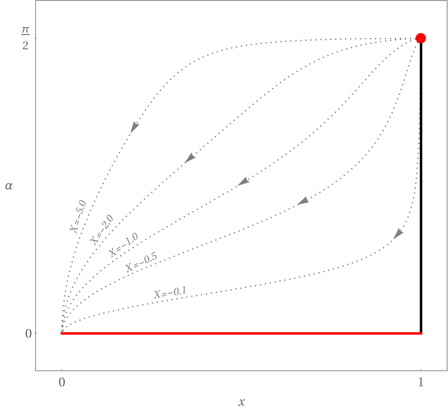 Figure 1
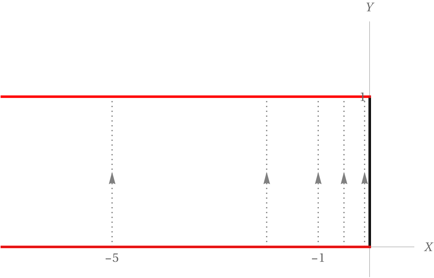 Figure 2
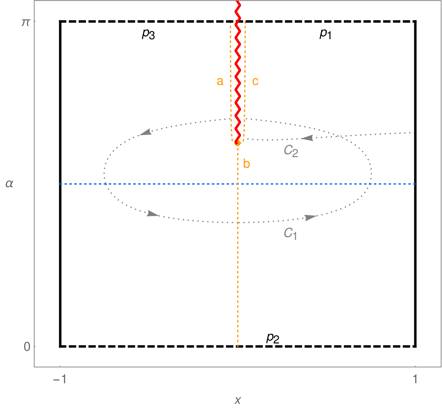 Figure 3
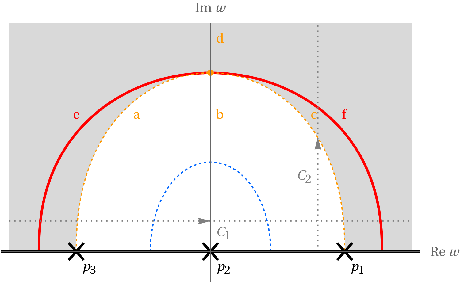 Figure 4
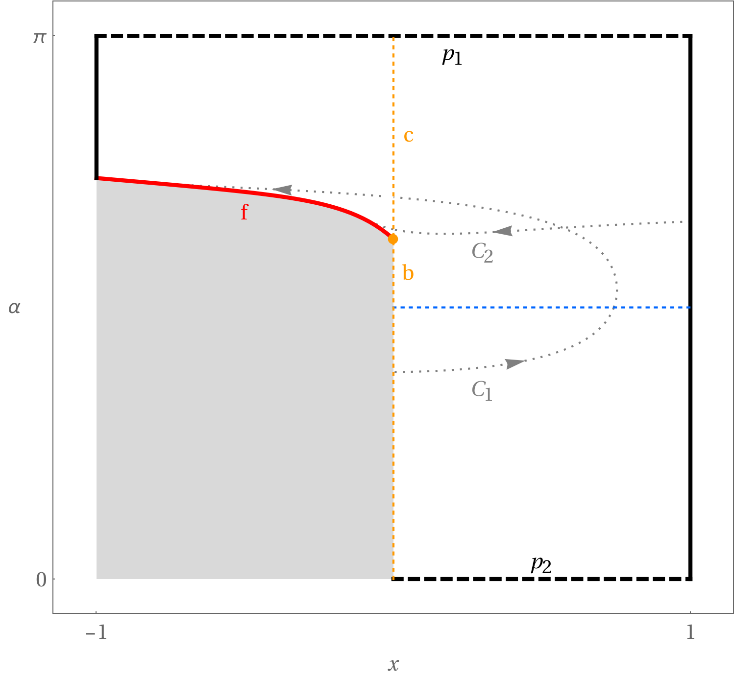 Figure 5
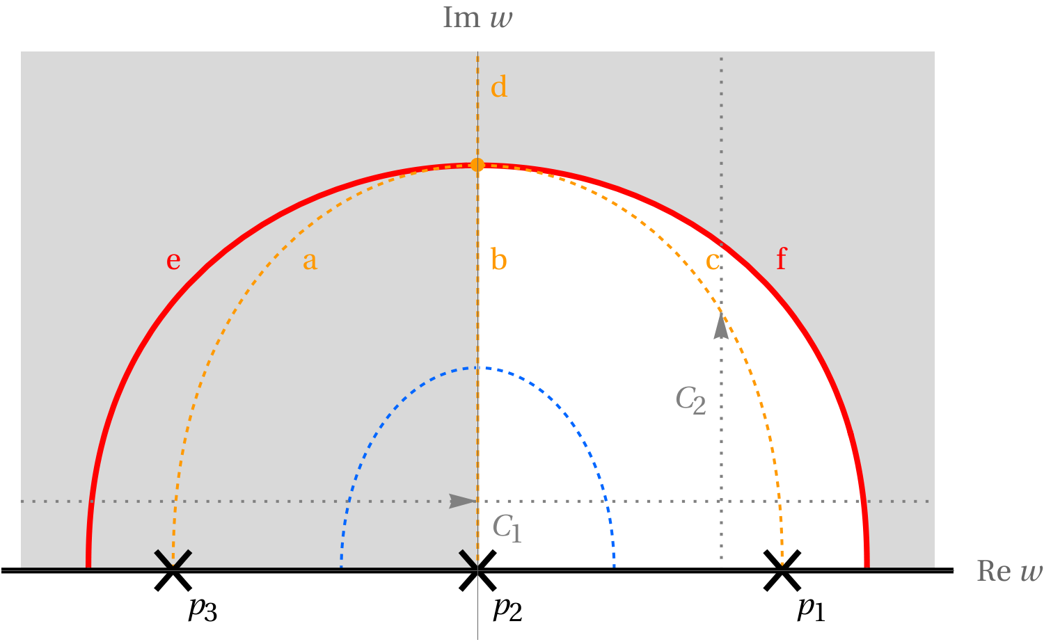 Figure 6
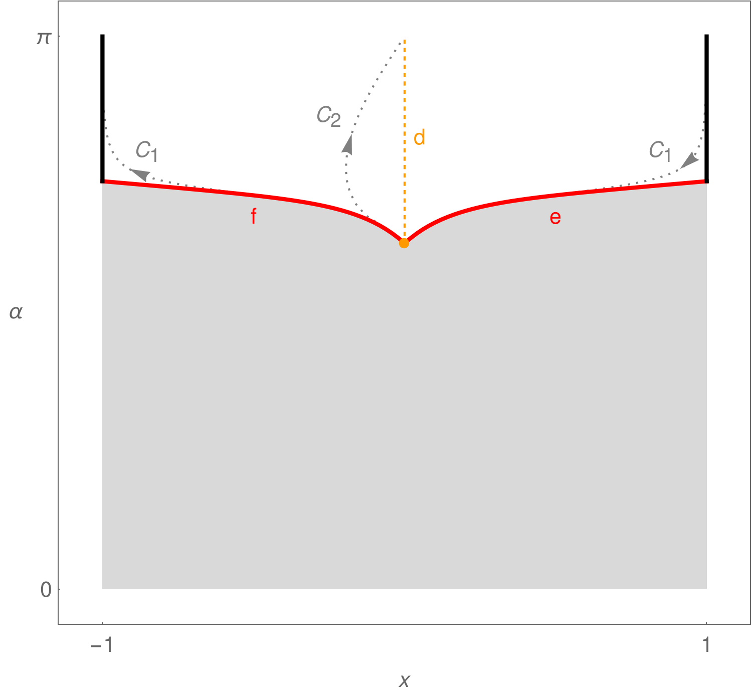 Figure 7
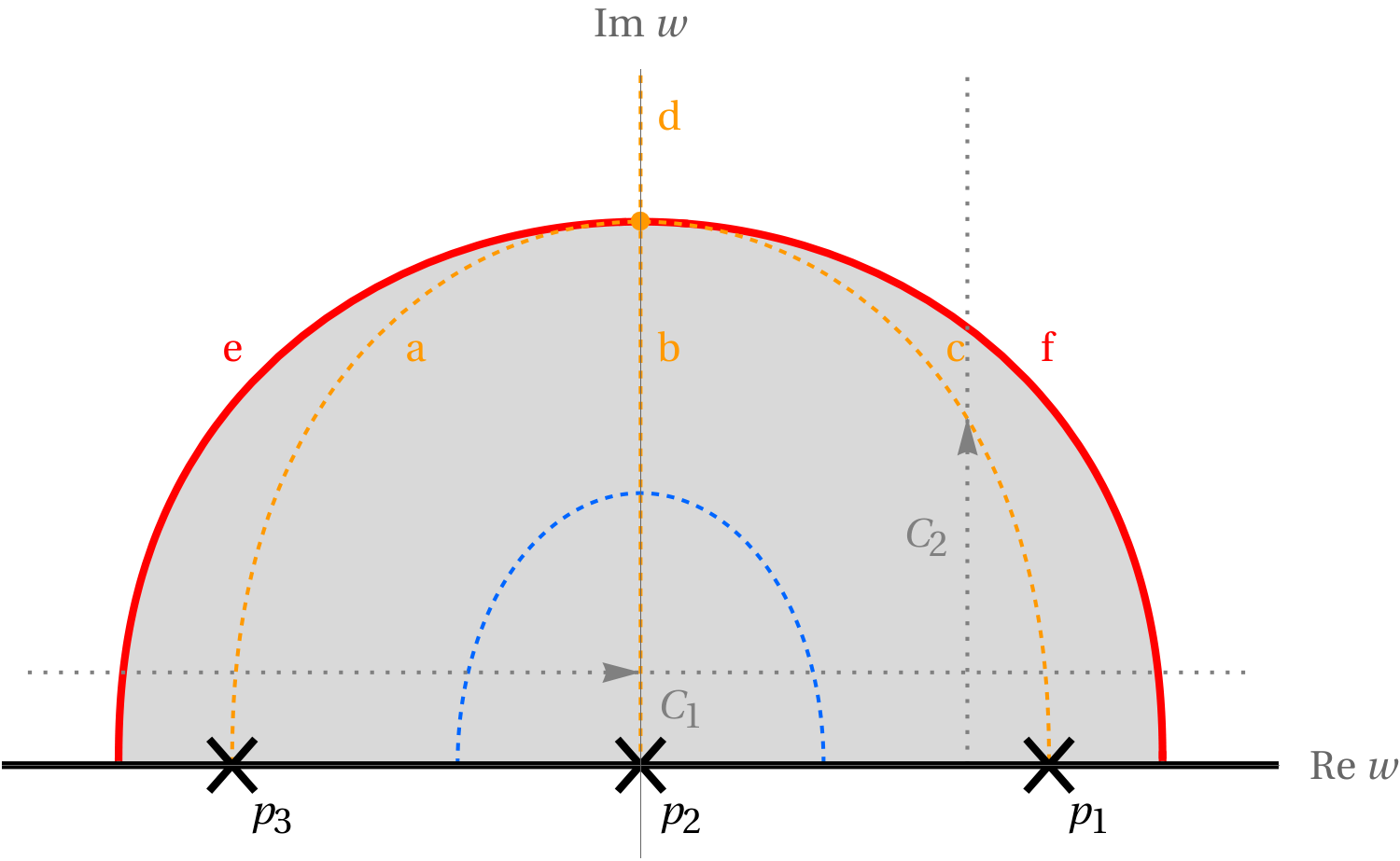 Figure 8
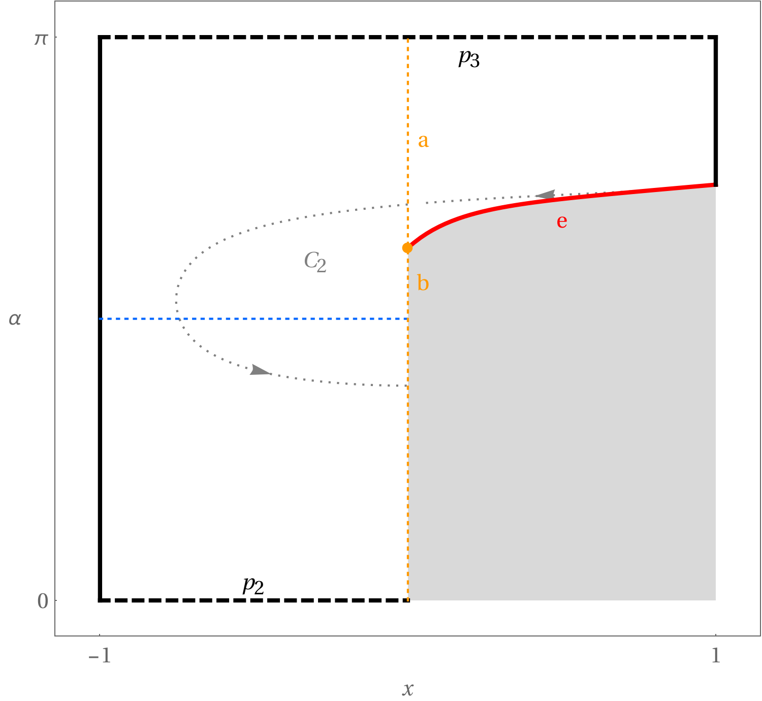 Figure 9
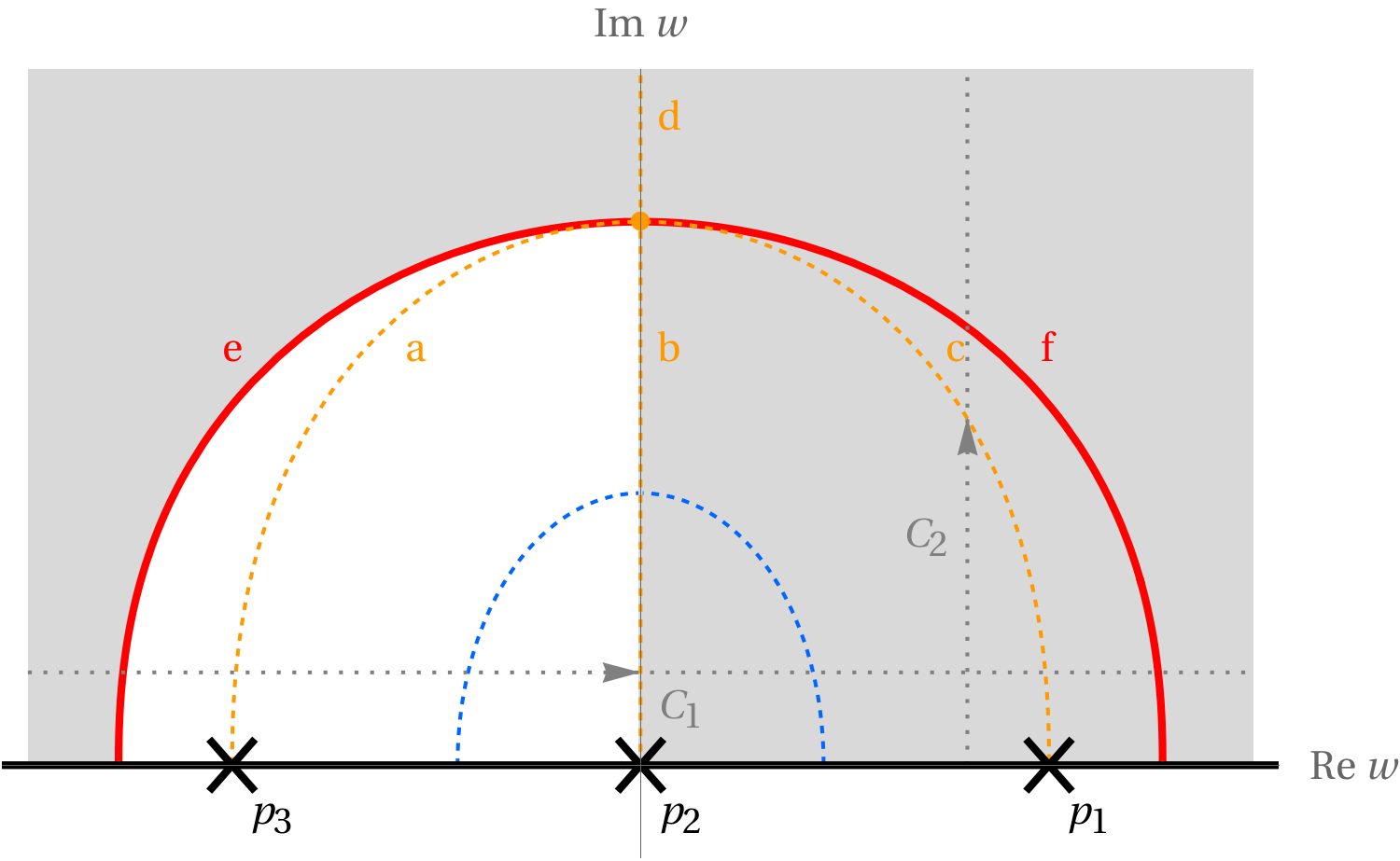 Figure 10
Peer Reviews
No public reviews on file for this paper yet. If you reviewed it on a platform where reviews are public (OpenReview, ICLR, NeurIPS, ICML), you can paste yours below so the community can read it here.
Videos
No videos yet. Explain this paper in a talk, walkthrough, or lecture? Add one.
January 30, 2019
Relating AdS6 solutions in type IIB supergravity
Kevin Chen and Michael Gutperle
*Mani L. Bhaumik Institute for Theoretical Physics
- *Department of Physics and Astronomy
University of California, Los Angeles, CA 90095, USA
[email protected], [email protected]
Abstract
In this note we show that the IIB supergravity solutions of the form AdS found by Apruzzi et al. in [1] are related to the local solutions found by D’Hoker et al. in [2]. We also discuss how the global regular solutions found in [3, 4] are mapped to the parameterization of [1].
1 Introduction
Five dimensional superconformal field theories take an interesting place among conformal field theories. They realize a unique superconformal algebra , they are strongly coupled in the UV, and many exhibit unusual properties such as enhanced exceptional flavour symmetries [5, 6, 7]. Holography is a useful method to study strongly coupled CFTs. However, until recently very few supergravity solutions in ten or eleven dimensions dual to five dimensional SCFTs were known. The first solutions [8, 9, 10] were constructed in massive IIA supergravity. Special examples of type IIB solutions were constructed from the type IIA solution using (non-Abelian) T-duality in [11, 12]. In [1] type IIB supergravity solutions were constructed from first principles. The solutions take the form of a fibration of AdS6 over a four dimensional base manifold and pure spinor geometry is used to determine the conditions for sixteen unbroken supersymmetries. It was found that the manifold is a fibration over a two dimensional space and the problem is reduced to solving two partial differential equations on this two dimensional space. In [2] a different approach utilizing Killing spinors on an AdS fibration over a two dimensional Riemann surface was used to reduce the BPS equations of the bosonic background. It was shown that local solutions can be expressed in terms of two holomorphic functions on the Riemann surface . Later, regular global solutions were constructed [3, 4] and shown to be related to the conformal fixed points of field theories derived from taking a conformal limit of 5-brane webs. Various aspects of these solutions have been studied recently, see e.g. [13, 14, 15, 16, 17, 18, 19, 20, 21, 22, 23, 24, 25].
The goal of the present note is to relate the form of the local IIB solutions found in [1] to the ones found in [2] and determine the exact map between the two. In addition we analyze the regularity conditions and the map for global regular solutions. The structure of the note is as follows. In sections 2 and 3 we briefly review the two supergravity solutions of [1] and [2] respectively. In section 4 we determine the exact map between these two solutions, and illustrate the relation with some explicit examples. In section 5, we look at how the global regular solution of [4] is mapped into framework of [1]. We conclude with a discussion in section 6.
2 Review of AFPRT solutions
Here we outline the solution in [1] by Apruzzi, Fazzi, Passias, Rosa, and Tomasiello (AFPRT). The spacetime takes the form of AdS and the supergravity fields depend on the two dimensional space through four quantities , two of which are actually independent and can be used to parameterize . Following [1] we take to be independent and and to be dependent functions. Here is a warping function and is the dilaton. These quantities satisfy two partial differential equations,
[TABLE]
The metric in the string frame is
[TABLE]
where are quantities defined by
[TABLE]
The one-form field strength is
[TABLE]
and the three-form NS-NS and R-R field strengths, and , are
[TABLE]
where and are signs and denotes the volume form of with unit radius. The self-dual five-form field strength vanishes in this background. These field strengths satisfy the Bianchi identities
[TABLE]
The signs depend on the specific supergravity solution, which we discuss later in this note.
3 Review of DGKU solutions
Here we outline the solution in [2] by D’Hoker, Gutperle, Karch, and Uhlemann (DGKU). The spacetime takes the form of AdS, where is a Riemann surface parametrized by complex coordinates . The supergravity fields depend only on through two holomorphic functions . For completeness we present the following quantities which are useful to express the supergravity fields in a concise form. We use the notation and .
[TABLE]
The metric in the Einstein frame is
[TABLE]
where the metric factors are
[TABLE]
Note that to make contact with the parameterization in section 2, the metric should be transformed into the string frame,
[TABLE]
Here the dilaton is normalized in the standard fashion to . The solution [2] utilizes an parametrization of the complex scalar field in terms of , which is related to the axion-dilaton field via
[TABLE]
and is given by [23] in terms of the defined quantities as
[TABLE]
where for notational convenience we introduced the quantities
[TABLE]
This gives expressions for the axion and the dilaton ,
[TABLE]
If we also define
[TABLE]
then noting the relations
[TABLE]
we have yet another expression for the axion and dilaton
[TABLE]
The one-form field strength is given in terms of the axion by
[TABLE]
The complex two-form potential is given by
[TABLE]
This can be written in terms of the real two-form potentials and ,
[TABLE]
where now
[TABLE]
This gives the R-R and NS-NS three-form field strengths and
[TABLE]
The self-dual five-form field strength vanishes. These field strengths satisfy the same Bianchi identities (2) given previously.
4 Mapping local solutions
Given these two different approaches to finding half-BPS solutions with factors in type IIB supergravity, our goal is to determine how they are related. We note that the difference in the parameterization of the solution lies in the two dimensional Riemann surface . The DGKU solution uses a uniformized form with complex coordinates whereas the AFPRT solution uses coordinates which are adapted to the pure spinor construction leading to the PDEs (2).
In order to relate the DGKU solution with the AFPRT solution the goal is to identify the four quantities of AFPRT in terms of the coordinates given the holomorphic data of DGKU. We use the fact that the four quantities are scalars with respect to and hence are independent of coordinate choices. Consequently they can be used to obtain a map between the two parameterizations. We show in the following that the coordinates and and the independent functions and can be expressed in terms of the holomorphic functions and that they satisfy the PDEs (2).
4.1 Positivity
We start by slightly adapting the discussion of positivity in [2]. On the Riemann surface , we consider solutions where the supergravity fields remain finite and the metric components are strictly positive:
[TABLE]
Then the definitions (3) imply that , , and are non-zero, finite, and have the same sign. From the definition of , we necessarily have . In taking the square-root we have a sign ambiguity, so without loss of generality we can take . This gives us the equivalent constraints
[TABLE]
4.2 Matching metric factors
We can start by identifying the metrical factors of and in the two string frame metrics (2.2) and (3.2).
[TABLE]
Then using the definitions in (3) we have
[TABLE]
The dilaton is given explicitly in Eq. (3), and so is through Eq. (4.2). Then including Eq. (4.4) above, we can express three quantities of AFPRT in terms of :
[TABLE]
Only one more quantity needs to be matched. If we equate the remaining portions of the two metrics, which correspond to , we can simplify to get
[TABLE]
We may also make the replacement . This equation turns out to be not very helpful because it contains derivatives of in . We can write the left-hand side in terms of , its first-order derivatives and , and other quantities we already know how to write in terms of . Matching the differentials , , and on both sides will give first-order non-linear PDEs for . We will not attempt this approach as it turns out there is a more direct way match the last remaining quantity.
4.3 Matching one-forms
The last remaining quantity can be matched using the one-form field strength. In AFPRT, is given in Eq. (2.4). In DGKU, we have an expression for the axion in Eq. (3.12). We can then simplify the equation to
[TABLE]
It is important to note that the dependence drops out. Now apart from , every quantity appearing in this equation (i.e. , , , and ) can be written in terms of . By making the replacement and squaring of both sides of the equation, we obtain a complex-valued quadratic equation for . This quadratic equation is very complicated for general functions, but will always have a real root with the surprisingly simple form
[TABLE]
This was arrived at by firstly taking explicit examples for where the one-form equation (4.6) was simple enough to be solved and guessing a general solution, and then verifying this solution algebraically for general using Mathematica. So far no insightful simplifications have been found; due to the simplicity of the solution despite the complexity of the quadratic equation, it is very possible that this conclusion can be obtained from simpler considerations. Another useful form is given by
[TABLE]
4.4 Explicit examples
Before continuing, let us verify this mapping for two established solutions which were discussed as examples in [1].
Example 1 – The first example of a type IIB solution in [1] is given by
[TABLE]
for . As the only independent variable is , this solution is slightly degenerate. The holomorphic data which reproduces this solution is given in [2], and is slightly changed here for convenience.
[TABLE]
Below we give some relevant derived quantities. In this example, we use coordinates .
[TABLE]
For positivity, we take . The one-form equation (4.6) simplifies to
[TABLE]
and has a solution . This is consistent with our solution for in Eq. (4.8) as has zero imaginary part. Then the equation for in Eq. (4.4) implies the coordinate change
[TABLE]
Plugging this into our expressions for and in (4.4) above gives exactly the desired solution (4.9), with the identifications
[TABLE]
If we write out the metric starting from (3.2) with , we can match the metric in [12, Eq. (A.1)] if we identify
[TABLE]
and the axion and dilaton if we identify
[TABLE]
where quantities with are those of [12]. Then the three-form field strengths and also match. In the literature, this solution is obtained by a Hopf -duality on the Brandhuber-Oz solution to massive IIA supergravity [8].
Example 2 – A second solution given in [1] is
[TABLE]
for and . The holomorphic data which reproduce this solution is
[TABLE]
Let us now try to rederive this AFPRT solution with this as our starting point. Below we give some relevant derived quantities. In this example, we use coordinates .
[TABLE]
For positivity, we take and . The one-form equation (4.6) has two solutions for : one complex-valued, which does not admit a simple expression, and one which coincides with our solution (4.8),
[TABLE]
Together, these imply the coordinate change
[TABLE]
This gives us the desired and with the identifications
[TABLE]
We can also match the metric, dilaton, and field strengths in [11, Eq. (11)] if we identify
[TABLE]
[TABLE]
where quantities with are those of [11]. Then the three-form field strengths and also match. In the literature, this solution is obtained by a non-Abelian -duality on the Brandhuber-Oz solution.
4.5 Summary of the relation
We have shown in this section the four quantities of AFPRT can be expressed in terms of the holomorphic functions of DGKU in the following way:
[TABLE]
We have verified that the map holds for two previously known solutions related to -duals of type IIA solutions. For general local solutions the algebra becomes very extensive. The following steps in verifying the map of DGKU to AFPRT have been performed algebraically for general using Mathematica:
Match the remaining parts of the metric corresponding to . Much of the work has already been done in (4.5), but now we are able to take derivatives on the left-hand side with relative ease. It also turns out quite nicely that and . 2. 2.
Match the three-form field strengths. We can check that the equations for and in the AFPRT solution match those of the DGKU solution. As our map only involves and , it does not distinguish between the signs of or . These signs are fixed by the sign convention
[TABLE]
Then the AFPRT three-form fields strengths in Eqs. (2) simplify to
[TABLE]
These are equivalent to those of DGKU in Eqs. (3). This means that in section 4.4, for Example 1 we take , and for Example 2 we take and . 3. 3.
Check the two PDEs. We can simplify the first PDE of (2) to
[TABLE]
while the second PDE has no significant simplification.
In summary we have shown that the general local DGKU solution can be mapped to the AFPRT parametrization and satisfies the PDEs (2) as a consequence of the holomorphy of the .
5 Mapping global solutions
After constructing a map from the local DGKU to AFPRT solutions, we now look at the global solutions constructed in [4]. They constitute a class of solutions (i.e. specified functions) where is taken to be the upper half-plane of the complex plane, whose boundary is the real axis. The have poles on the boundary. The geometry is completely regular everywhere, except for the location of the poles where the supergravity background becomes that of a five-brane. The supergravity solution can be viewed as the conformal near horizon limit of a five-brane web and the poles are interpreted as the residues of the semi-infinite external five-branes framing the web. If we take to be alternative coordinates of , we can ask how these features are mapped over. We will find that while these global solutions are represented by a single coordinate patch on the complex plane, mapping over to the -coordinates requires multiple coordinate patches in order to have single-valued supergravity fields.
For simplicity we define
[TABLE]
In particular, this means . Then as by definition, the square
[TABLE]
becomes a very natural coordinate system for . We will adopt this coordinate system for this section.
5.1 Boundary conditions
We are mainly interested in solutions where the AdS6 factor governs the entire non-compact part of the geometry. Therefore, we will assume that is compact, with or without boundary. On a non-empty boundary , we enforce while keeping the other conditions the same. Physically, this corresponds to shrinking the sphere closing off the geometry and forming a regular three-cycle which carries the five brane charges. This is equivalent to the boundary conditions
[TABLE]
The constraint is relaxed at isolated points on the boundary to allow for sufficiently mild singularities, such as at the poles corresponding to five-branes.
We can now make some general remarks on the boundary . As we have . From the definition of in Eqs. (3), we also have . Therefore
[TABLE]
Thus is fixed, but because is non-zero and finite (away from the five-brane poles), can take generic values on the interval . Therefore we can say that the boundary corresponds to (segments of) the edges of the square. Note that the boundary may not necessarily be mapped to the entire edge , but can map to just a segment of the edge.
5.2 Example: non-Abelian -dual
As a warm-up, let us return to the second example of section 4.4, with and for concreteness. We will first identify the Riemann surface on the complex plane, and then see how this region maps into the square. Recall that .
[TABLE]
We satisfy on the semi-infinite strip and , which we take to be . Additionally, on the line segment and , which we take to be the boundary . The semi-infinite lines at and are then coordinate singularities, where various metric components blow up.
[TABLE]
The coordinate patch for on the complex plane is shown in figure 1(a). The black line represents the boundary , and the red lines represent the coordinate singularities.
The coordinate change, given in Eq. (4.4), maps this semi-infinite strip on the complex plane into the quadrant of the square. Explicitly,
[TABLE]
Features of this map are shown in figure 1. The boundary maps onto the line segment as expected. We have also included contours for visual aid, represented by dotted gray lines. On the left-hand side we have drawn some contours of constant , and on the right-hand side we show their images in the -coordinates.
5.3 Example: 3-pole global solution
Let us finally turn our attention to the global solutions. We summarize the relevant details from [4] for the general case of poles, and then specialize to a concrete example of three poles.
Take to be the upper half-plane of the complex plane, and to be the real-axis. Let be the locations of poles on the real-axis, and be the locations of zeros strictly in the upper half-plane, where . Then let
[TABLE]
where for are constants defined by
[TABLE]
and is a complex-valued normalization constant.111In terms of the original paper, where and . If we integrate the expressions for , we have
[TABLE]
where is a constant satisfying the equation below for .
[TABLE]
This makes and vanish on the real-axis, according to the usual definitions in (3) after some consideration of branch cuts. contains dilogarithms, so any quantity containing it in undifferentiated form (such as ) will not admit a simple form. However, near a pole we can look at the asymptotic behavior. Let us consider a pole and take the semi-circle , where and for all . Then we have the following relevant leading behaviors:
[TABLE]
where
[TABLE]
so that near a pole as
[TABLE]
Therefore, small semi-circles around a pole on the complex plane map to lines of constant on the square, which approach either the or edge as . Because is approximately , these semi-circles necessarily map to the entire line segment running between . This can all be loosely summarized by saying poles on the boundary correspond to the edges of the square.
For concreteness let us take the 3-pole solution, which is the simplest global solution with the fewest number of poles. We pick the locations of the three poles,
[TABLE]
the location of the one zero,
[TABLE]
and the normalization constant,
[TABLE]
The relations (5.11) are solved by .
This defines a coordinate change from the upper half-plane into the square . This map does not admit a simple form as it contains dilogarithms, but its general features are shown in figure 2. The left-hand diagrams show an unshaded region on the complex plane, and the right-hand diagrams show the corresponding region on the square. Solid black lines represent the boundary . “X” marks on the complex plane represent locations of the five-brane poles, which map to black dashed lines on the square. Two contours are included for visual aid.
There are three important considerations which make this map well-defined:
For convenience, we pick a map which obeys the sign convention (4.25) with . On the complex plane, we have represented the curve where with an orange dotted line. This curve is mapped to . The side of the curve where gets mapped to the side of the square, and the side where gets mapped to . Similarly, the curve where is represented with a blue dotted line.222 also vanishes on the boundary , but we exclude this. 2. 2.
In order to map the entire upper half-plane of the complex plane into -coordinates in a one-to-one manner, we need to introduce multiple coordinate patches. This follows from a simple counting argument: each of the three poles needs to be mapped their own or edge, only two of which exist on the square. We can accommodate a one-to-one map at the expense of introducing multiple squares and gluing them together.
For instance, the pole maps to the edge, and the boundary segments and map to the and edges, respectively. The and poles then map to the edge of two different squares 2(d) and 2(h), respectively. These two patches are glued together along the orange line “b”. Figure 2(b) shows these two patches glued together at the expense of introducing a branch cut, represented by the red jagged line. 3. 3.
The Jacobian of the map vanishes on the solid red line.
[TABLE]
In the present example, if a contour on the complex plane passes through this line, the image of the contour in -coordinates will instead bounce off this line. This means that we need an additional coordinate patch to maintain a one-to-one map. For instance, consider the contour in -coordinates: it starts on the coordinate patch 2(d), hits the red line “f”, and then bounces off onto another coordinate patch 2(f).
To summarize, is represented on the complex plane by a single coordinate patch, taken to be the upper half-plane. When we map over to -coordinates, we need at least three coordinate patches to represent the whole : 2(d), 2(f), and 2(h). 2(d) is glued to 2(h) along “b”, 2(d) to 2(f) along “f”, and 2(f) to 2(h) along “e”.
6 Discussion
In this note we have found an explicit map between the type IIB AdS6 solutions formulated in [1] and in [2]. This mapping is given by a coordinate change for the surface and was explicitly verified for two previously known examples. This result shows that the two solutions are indeed equivalent and that therefore the solutions of [2] are the most general type IIB solutions with an AdS6 factor preserving sixteen supersymmetries.
Furthermore we mapped over the global solutions of [4] and found that multiple coordinate patches in were necessary in order to have single-valued solution. This arose from a simple counting argument that each five-brane pole of the global solution needs to be mapped to its own horizontal edge of the coordinate square, but global solutions have poles whereas each square has 2 horizontal edges. Thus an advantage of the complex coordinate parametrization of [2] is that a global solution can be represented in a single coordinate chart. Note that in [1] the four quantities are initially on the treated same footing and subsequently are chosen to be coordinates of the two dimensional space . It is an interesting open question whether the global solutions can be formulated by making different coordinate choices.
In [26, 27] the AFPRT solution was reduced on AdS6 and an effective scalar coset theory was constructed. The symmetries of the coset can be used to generate new solutions. It would be interesting to investigate how the coset transformations act on the DGKU solutions using the mapping constructed in the present paper. Another interesting direction would be to see how the alternative formulation in [28] can be related to the DKGU solutions.
Acknowledgements
We are grateful to Christoph Uhlemann for useful conversations. The work of M. G. is supported in part by the National Science Foundation under grant PHY-16-19926.
The reference list from the paper itself. Each links out to its DOI / PubMed record.
- 1[1] F. Apruzzi, M. Fazzi, A. Passias, D. Rosa and A. Tomasiello, Ad S 6 solutions of type II supergravity , JHEP 11 (2014) 099 [ 1406.0852 ]. · doi ↗
- 2[2] E. D’Hoker, M. Gutperle, A. Karch and C. F. Uhlemann, Warped A d S 6 × S 2 𝐴 𝑑 subscript 𝑆 6 superscript 𝑆 2 Ad S_{6}\times S^{2} in Type IIB supergravity I: Local solutions , JHEP 08 (2016) 046 [ 1606.01254 ]. · doi ↗
- 3[3] E. D’Hoker, M. Gutperle and C. F. Uhlemann, Holographic duals for five-dimensional superconformal quantum field theories , Phys. Rev. Lett. 118 (2017) 101601 [ 1611.09411 ]. · doi ↗
- 4[4] E. D’Hoker, M. Gutperle and C. F. Uhlemann, Warped A d S 6 × S 2 𝐴 𝑑 subscript 𝑆 6 superscript 𝑆 2 Ad S_{6}\times S^{2} in Type IIB supergravity II: Global solutions and five-brane webs , JHEP 05 (2017) 131 [ 1703.08186 ]. · doi ↗
- 5[5] N. Seiberg, Five-dimensional SUSY field theories, nontrivial fixed points and string dynamics , Phys. Lett. B 388 (1996) 753 [ hep-th/9608111 ]. · doi ↗
- 6[6] D. R. Morrison and N. Seiberg, Extremal transitions and five-dimensional supersymmetric field theories , Nucl. Phys. B 483 (1997) 229 [ hep-th/9609070 ]. · doi ↗
- 7[7] K. A. Intriligator, D. R. Morrison and N. Seiberg, Five-dimensional supersymmetric gauge theories and degenerations of Calabi-Yau spaces , Nucl. Phys. B 497 (1997) 56 [ hep-th/9702198 ]. · doi ↗
- 8[8] A. Brandhuber and Y. Oz, The D-4 - D-8 brane system and five-dimensional fixed points , Phys. Lett. B 460 (1999) 307 [ hep-th/9905148 ]. · doi ↗